SOFIA FORCAST photometry of 12 Extended Green Objects in the Milky Way

SOFIAFORCASTPHOTOMETRY OF 12 EXTENDED GREEN OBJECTS IN THE MILKY WAY

A. P. M. TOWNER1*,2, C. L. BROGAN1, T. R. HUNTER1, C. J. CYGANOWSKI3, R. K. FRIESEN1

Draft version March 19, 2019

ABSTRACT

Massive young stellar objects are known to undergo an evolutionary phase in which high mass accretion rates drive strong outflows. A class of objects believed to trace this phase accurately is the GLIMPSE Extended

Green Object (EGO) sample, so named for the presence of extended 4.5µm emission on sizescales of∼0.1

pc in Spitzerimages. We have been conducting a multi-wavelength examination of a sample of 12 EGOs

with distances of 1 to 5 kpc. In this paper, we present mid-infrared images and photometry of these EGOs obtained with the SOFIA telescope, and subsequently construct SEDs for these sources from the near-IR to sub-millimeter regimes using additional archival data. We compare the results from greybody models and several publicly-available software packages which produce model SEDs in the context of a single massive

protostar. The models yield typicalR?∼10R,T?∼103to 104K, andL?∼1−40×103L; the medianL/M

for our sample is 24.7L/M. Model results rarely converge forR?andT?, but do forL?, which we take to be

an indication of the multiplicity and inherently clustered nature of these sources even though, typically, only a

single source dominates in the mid-infrared. The medianL/Mvalue for the sample suggests that these objects

may be in a transitional stage between the commonly described “IR-quiet” and “IR-bright” stages of MYSO

evolution. The medianTdustfor the sample is less conclusive, but suggests that these objects are either in this

transitional stage or occupy the cooler (and presumably younger) part of the IR-bright stage.

Subject headings:stars: formation stars: massive stars: protostars infrared: general radiative transfer

-techniques: photometric

1. INTRODUCTION

Massive young stellar objects (MYSOs) are challenging to observe due to their comparative rarity and short-lived na-tal phase, large distances from Earth, and highly-obscured

formation environments. Early observations of suspected

MYSOs were performed mostly with large beams, and probed

size scales ranging from cores to clumps and clouds (∼0.1 pc,

∼1 pc, and ∼10 pc, respectively; see Kennicutt & Evans

2012). Detailed descriptions of early surveys for MYSOs and their results can be found in, e.g., Molinari et al. (1996), Sridharan et al. (2002), and Fontani et al. (2005). Follow-up observations with improved sensitivity and spatial reso-lution, such as interferometric radio and millimeter obser-vations, revealed that many of the objects originally identi-fied as “MYSOs” were actually sites in which multiple pro-tostars were forming simultaneously (e.g. Hunter et al. 2006; Cyganowski et al. 2007; Vig et al. 2007; Zhang et al. 2007, to name just a few). This predilection for forming in clustered environments means that the study of high-mass protostars is

necessarily the study of protoclusters: clusters of protostars

with a range of masses and in a variety of evolutionary stages. Current theories of high mass star formation differ in their predictions of the aggregate properties of these protoclusters, such as mass segregation (if any), sub-clustering of the pro-tostars, and stellar birth order (e.g. Vázquez-Semadeni et al. 2017; Banerjee & Kroupa 2017; Bonnell & Bate 2006; Mc-Kee & Tan 2003). It is therefore necessary to consider each

1_{National Radio Astronomy Observatory, 520 Edgemont Rd,} Char-lottesville, VA 22903, USA

2_{Department of Astronomy, University of Virginia, P.O. Box 3818,} Charlottesville, VA 22903, USA

3_{Scottish Universities Physics Alliance (SUPA), School of Physics and} Astronomy, University of St. Andrews, North Haugh, St Andrews, Fife KY16 9SS, UK

*_{A.P.M.T. is a Grote Reber Doctoral Fellow at the National Radio} As-tronomy Observatory.

high-mass protostar in combination with its environment. Extended Green Objects (EGOs) were first identified by Cyganowski et al. (2008) using data from the Galactic Legacy Infrared Midplane Survey Extraordinaire (GLIMPSE, Ben-jamin et al. 2003; Churchwell et al. 2009) project. EGOs

are named for their extended emission in the 4.5µmSpitzer

IRAC band (commonly coded as “green” in three-color RGB

images), which is due to shocked H2 from powerful

proto-stellar outflows (e.g., Marston et al. 2004). Follow-up

obser-vations of ∼20 EGOs with the Karl G. Jansky Very Large

Array (VLA) by Cyganowski et al. (2009) established both the presence of massive protostars (traced by 6.7 GHz Class

II CH3OH masers) and shocked molecular gas indicative of

outflows (traced by 44 GHz Class I CH3OH masers). The

causal link between accretion and ejection (Frank et al. 2014) thus implies that these objects contain protostars undergoing active accretion, and the maser data indicate that these proto-stars are massive. The youth of the massive protoproto-stars within these EGOs was confirmed by deep (at that time) VLA contin-uum observations (Cyganowski et al. 2011b), which yielded only a few 3.6 cm detections, and by later VLA 1.3 cm con-tinuum observations (Towner et al. 2017), which revealed

pri-marily weak (<1 mJy beam−1), compact emission. The low

detection rates and integrated flux densities of the centime-ter continuum emission in these sources demonstrate that any free-free emission is weak, consistent with a stage prior to the development of ultracompact HII regions.

Given that high-mass stars form in clusters, it is likely that EGOs are signposts for protoclusters rather than isolated high-mass protostars, though the level of multiplicity of

mas-sive sources (>8M) and overall cluster demographics

re-main open questions. Millimeter dust continuum

observa-tions of EGOs with∼300resolution, suggest that the number

of massive protostars per EGO is typically one to a few (e.g. Cyganowski et al. 2012, 2011a; Brogan et al. 2011).

ever, the precise physical properties of protoclusters traced by EGO emission - such as total mass, luminosity, and massive protostellar multiplicity - remain largely unexplored in EGOs as a class.

The infrared emission from EGOs, and indeed MYSOs in general, is often challenging to characterize due to the pres-ence of high extinction from their surrounding natal clumps (as they are still deeply embedded), and confusion from more evolved sources nearby. The latter issue has been particularly affected by the relatively poor angular resolution (>10) that has heretofore been available at mid- and far-infrared wave-lengths, where the high extinction can be overcome. Yet these wavelengths contain crucial information as hot dust, shocked gas, and polycyclic aromatic hydrocarbons (PAHs) all emit in this regime. Scattered light originating from the protostar it-self may also sometimes escape through outflow cavities and would likewise be visible in the infrared. Thus mid-infrared wavelengths are a crucial component of the Spectral Energy Distribution (SED) which is a useful tool for constraining im-portant source properties such as mass, bolometric luminosity, and temperature.

These properties are of particular interest for MYSOs, as re-cent analysis of the Herschel InfraRed Galactic Plane Survey (Elia et al. 2017) and a full census of the properties of ATLAS-GAL Compact Source Catalog (CSC) objects Urquhart et al.

(2018) shows how the luminosity to mass ratioL/Mof

proto-stellar clumps can be used to both qualitatively and quantita-tively discriminate between the different evolutionary stages

of pre- and protostellar objects. In theoretical terms,L/M is

tied to evolutionary state primarily due to abrupt changes in luminosity during different stages of MYSO/clump evolution (see, e.g., the stages described in Hosokawa & Omukai 2009; Molinari et al. 2008).

In this paper, we present new data that directly address the questions of the multiplicity and physical properties (tem-perature, mass, and luminosity) of the massive protoclus-ters traced by EGOs. We have utilized the unique capabili-ties of the Stratospheric Observatory for Infrared Astronomy (SOFIA, Temi et al. 2014) to image a well-studied sample of

12 EGOs at two mid-IR wavelengths: 19.7 and 37.1µm with

the necessary sensitivity (∼0.05 to∼0.25 Jy beam−1) and an-gular resolution (∼300) to detect and resolve the mid-infrared emission from the massive protocluster members. By com-bining these results with ancillary multi-wavelength archival data, we create well-constrained SEDs from the near-infrared through submillimeter regimes. We then use three SED mod-elling packages published by Robitaille et al. (2006), Ro-bitaille (2017), and Zhang & Tan (2018), to constrain phys-ical parameters (see, e.g., Gaczkowski et al. 2013; De Buizer et al. 2017). In § 2, we describe our targeted SOFIA observa-tions and the observational details of the archival data at each wavelength. In § 3, we describe our aperture-photometry pro-cedures for each data set and discuss our detection rates and trends. We also present sets of multi-scale, multiwavelength images for each object in order to better demonstrate their small- and large-scale properties and overall environments. In § 4, we compare the physical parameters obtained from the

various SED modeling methods, includingL/M, which help

to place EGOs into a broader evolutionary context. In § 5 we discuss the implications of our results, and outline future investigations.

2. THE SAMPLE & OBSERVATIONS

In this paper, we conduct a multiwavelength aperture-photometry study of 12 EGOs using the SOFIA Faint Ob-ject infraRed CAmera for the SOFIA Telescope (FORCAST

Herter et al. 2012). We use new SOFIA FORCAST

19µm and 37µm observations in conjunction with

publicly-available archival datasets fromSpitzer,Herschel, and the

At-acama Pathfinder EXperiment5 _{(APEX) telescope, to model}

the SED of the dominant protostar in each of our target EGOs. Details of source properties for our sample are listed in Ta-ble 1.

2.1. SOFIA FORCAST Observations: 19.7 & 37.1µm

We used SOFIA FORCAST to observe our 12 targets

si-multaneously at 19.7µm and 37.1 µm. Observations were

performed in the asymmetric chop-and-nod imaging

observ-ing mode C2NC2. The measured6FWHM are 2.00_{5 at 19.7µm}

and 3.004 at 37.1µm. At the nearest (1.13 kpc) and farthest

(4.8 kpc) source distances, these FWHM correspond to

phys-ical size scales of 2,830 to 12,000 au at 19.7µm and 3,840 to

16,300 au at 37.1µm. The instantaneous field of view (FOV)

of FORCAST is 3.04×3.02, with pixel sizeθ = 0.00768 after

distortion correction. This FOV corresponds to 1.1×1.1 pc

at a distance of 1.13 kpc, and 4.8×4.5 pc at a distance of 4.8

kpc. Table 2 summarizes observation information for each EGO. The project’s Plan ID is 04_0159.

Data calibration and reduction are performed by the SOFIA

team using the SOFIA data-reduction pipeline7_{. After}

re-ceipt of the Level 3 data products (artifact-corrected,

flux-calibrated images), we converted our images from Jy pixel−1

to Jy beam−1 in order to more easily perform photometric

measurements in CASA (McMullin et al. 2007).

Conver-sion was accomplished by using the CASA taskimmathto

multiply each image by the beam-to-pixel conversion factor

Xλ= (beam area)/(pixel area). This factor depends on beam

size and pixel size, and therefore is different for each

wave-length. The beam-to-pixel conversion factors are X19.7µm=

12.0067 pixels/beam and X37.1µm= 22.2076 pixels/beam.

2.2. Archival Data

2.2.1. Spitzer IRAC (GLIMPSE) Observations: 3.6, 5.8, & 8.0µm

All of our EGO targets were originally selected due to their

extended emission at 4.5 µm as seen in SpitzerGLIMPSE

images. In order to constrain the SEDs of the driving

sources themselves, we used the archival Spitzer

observa-tions at 3.6 µm, 5.8 µm, and 8.0 µm (bands I1, I3, and

I4, respectively) from the GLIMPSE project (Benjamin et al. 2003; Churchwell et al. 2009). The point response function (PRF) of the IRAC instrument varies by band and position on the detector. The mean FWHM in bands I1, I3, and I4 are 1.0066, 1.0072, and 1.0088, respectively, as detailed in Fazio et al. (2004). All archival GLIMPSE data were downloaded from the NASA/IPAC Infrared Science Archive (IRSA) Gator

Cat-5_{This publication is based on data acquired with the Atacama Pathfinder} Experiment (APEX). APEX is a collaboration between the Max-Planck-Institut fur Radioastronomie, the European Southern Observatory, and the Onsala Space Observatory.

6 _{These FWHM are the average values in dual-channel mode for each} wavelength as measured by the SOFIA team since Cycle 3. More information can be found in the Cycle 5 Observer’s Handbook on the SOFIA website at https://www.sofia.usra.edu/science/proposing-and-observing/sofia-observers-handbook-cycle-5

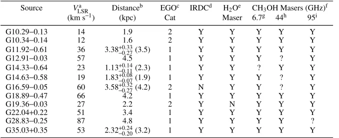
TABLE 1 EGO SOURCEPROPERTIES

Source V_LSRa Distanceb _EGOc _IRDCd _H

2Oe CH3OH Masers (GHz)f (km s−1_{) (kpc) Cat Maser 6.7}g ₄₄h ₉₅i

G10.29−0.13 14 1.9 2 Y Y Y Y Y

G10.34−0.14 12 1.6 2 Y Y Y Y Y

G11.92−0.61 36 3.38+0.33

−0.27(3.5) 1 Y Y Y Y Y

G12.91−0.03 57 4.5 1 Y Y Y ? Y

G14.33−0.64 23 1.13+0.14

−0.11(2.3) 1 Y Y ? Y Y

G14.63−0.58 19 1.83+0.08

−0.07(1.9) 1 Y Y Y ? Y

G16.59−0.05 60 3.58+0.32

−0.27(4.2) 2 N Y Y ? Y

G18.89−0.47 66 4.2 1 Y Y Y Y Y

G19.36−0.03 27 2.2 2 Y N Y Y Y

G22.04+0.22 51 3.4 1 Y Y Y Y Y

G28.83−0.25 87 4.8 1 Y Y Y Y ?

G35.03+0.35 53 2.32+0.24

−0.20(3.2) 1 Y Y Y Y Y

a_{LSRK velocities are the single dish NH}

3(1,1) values from Cyganowski et al. (2013).

b_{Distances without errors are estimated from the LSRK velocity and the Galactic rotation curve} param-eters from Reid et al. (2014). Parallax distances (with their uncertainties) are given where available from Reid et al. (2014) and references therein, with the kinematic distance in parentheses for comparison. All kinematic distances are the near distance. The uncertainty on each kinematic distance is assumed to be 15%, based on the median percent difference between the parallax-derived and kinematic distances from the five sources which have both.

c_{This is the Table number of the EGO in Cyganowski et al. (2008). In that paper, Tables 1 & 2 list} “likely” EGOs for which 5-band (3.6 to 24µm) or only 4.5µmSpitzerphotometry can be measured, respectively.

d_{Coincidence of EGO with IRDC as indicated by Cyganowski et al. (2008).}

e_{Water maser data from the Cyganowski et al. (2013) Nobeyama 45-m survey of EGOs.} f_{Sources for which we could find no information in the literature are indicated by “?".}

g _{The 6.7 GHz maser detection information comes from Cyganowski et al. (2009) using the VLA,} except for G12.91−0.03, G14.63−0.58, and G16.59−0.05, which come from Green et al. (2010, and references therein) observations using the Australia Telescope Compact Array (ATCA).

h_{Information for 44 GHz masers come from the VLA and were taken from Cyganowski et al. (2009),} except for G14.33−0.64, which comes from Slysh et al. (1999).

i_{Most information for 95 GHz masers was taken from Chen et al. (2011) using the Mopra 22 m} tele-scope. The exceptions are G14.33−0.64 from Val’tts et al. (2000) using Mopra, G16.59−0.05 from Chen et al. (2012) using the Purple Mountain Observatory 13.7 m telescope, and G35.03+0.35 from Kang et al. (2015) using the Korean VLBA Network.

TABLE 2

SOFIA FORCAST OBSERVINGPARAMETERS

Source Pointing Center (J2000) Obs. Datea _TOSb _σ(MAD)c

RA Dec (s) 37µm 19µm

G10.29−0.13 18:08:49.2 -20:05:59.3 2016 July 13 502 0.26 0.08

G10.34−0.14 18:08:59.9 -20:03:37.3 2016 Sept 27 626 0.30 0.07 G11.92−0.61 18:13:58.0 -18:54:19.3 2016 July 12 604 0.22 0.07 G12.91−0.03 18:13:48.1 -17:45:41.3 2016 July 19 1000 0.18 0.04 G14.33−0.64 18:18:54.3 -16:47:48.3 2016 July 12 593 0.24 0.07 G14.63−0.58 18:19:15.3 -16:29:57.3 2016 July 13 641 0.22 0.07 G16.59−0.05 18:21:09.0 -14:31:50.3 2016 July 20 810 0.19 0.04 G18.89−0.47 18:27:07.8 -12:41:38.3 2016 Sept 27 626 0.25 0.06 G19.36−0.03 18:26:25.7 -12:03:56.3 2016 Sept 20 285 0.46 0.09 G22.04+0.22 18:30:34.6 -09:34:49.3 2016 Sept 20 642 0.21 0.05 G28.83−0.25 18:44:51.2 -03:45:50.3 2016 Sept 27 470 0.26 0.07 G35.03+0.35 18:54:00.4 +02:01:15.7 2016 Sept 22 500 0.29 0.08 a_{All July observations were performed on flights from Christchurch, New Zealand; all September}

observations were performed on flights from Palmdale, CA, USA.

b_{This column lists the total time on source (TOS) for each target. The original proposal called for}

600 s of integration on each source. For four sources, 600 s could not be achieved due to either high clouds (G19.36) or telescope issues (G10.29, G28.83, G35.03). G12.91 was a shared observation with another group whose observations required additional integration time.

c_{The background noise of the SOFIA images is non-Gaussian in the majority of sources. This column}

alog List. The images returned by the archive are all in units of MJy sr−1_.

2.2.2. Spitzer MIPS (MIPSGAL) Observations: 24µm

We utilized archival 24µm data from the MIPSGAL survey

to provide additional mid-IR constraints on our SEDs for 9 of our 12 targets. For the remaining 3 targets (G14.33, G16.59,

G35.03), MIPSGAL 24µm data could not be used for the

second task due to saturated pixels in the regions of interest.

MIPSGAL images have a native brightness unit of MJy sr−1_,

and were converted to Jy beam−1 by first multiplying each

image by 1×106_{(to convert from MJy to Jy) and then}

multi-plying by the solid angle subtended by the 6.000×6.000 MIPS

beam at 24µm. Technical details of the MIPS instrument can

be found in Rieke et al. (2004). For details of the MIPSGAL observing program, see Carey et al. (2009) and Gutermuth & Heyer (2015). All MIPSGAL data were downloaded from the IRSA Gator Catalog List.

2.2.3. Herschel PACS (Hi-GAL) Observations: 70 & 160µm

We used archival 70µm and 160 µm data from the

Her-schel Infrared Galactic Plane Survey (Hi-GAL, Molinari et

al. 2016), observed with theHerschelPhotoconductor Array

Camera and Spectrometer (PACS; Poglitsch et al. 2010) in-strument, to probe the far-IR portion of the spectrum. These data were originally observed as part of the Herschel Hi-GAL project (Molinari et al. 2010, 2016) between 2010 Oc-tober 25 and 2011 November 05. The observations were

per-formed in parallel mode with a scan speed of 6000/s. Beam

sizes, which are dependent on observing mode, wereθ70µm=

5.800×12.100andθ160µm= 11.400×13.400as reported in Moli-nari et al. (2016). The native brightness unit of the Hi-GAL

data is MJy sr−1. Therefore, these images were converted to

Jy beam−1using the same method as in §2.2.2.

We chose to use the Hi-GAL data over the archival PACS data available on the European Space Agency (ESA) Her-itage Archive due to the additional astrometric and absolute flux calibration performed by the Hi-GAL team, as detailed in Molinari et al. (2016). All Hi-GAL data were obtained from the Hi-GAL Catalog and Image Server on the Via Lactea web portal8_.

2.2.4. APEX LABOCA (ATLASGAL) Observations: 870µm

We used archival 870 µm observations from the APEX

Telescope Large Area Survey of the Galaxy (ATLASGAL, Schuller et al. 2009) to populate the submillimeter portion of the SED. The data were retrieved from the ATLASGAL

Database Server9_{. The ATLASGAL beam size is 19.}00₂

× 19.002; additional observational details can be found in

Schuller et al. (2009). These images were already in units

of Jy beam−1_{, and thus required no unit conversion.}

3. RESULTS

Figures 1 through 4 show pairs of three-color (RGB)

im-ages for each source. The left-hand panels show a 5.03 field

of view with 160, 70, and 24µm data mapped to R, G, and

B, respectively, and with 870µm contours overlaid. These

panels show the large-scale structure of the cloud and over-all environment in which each EGO is located. The

right-hand panels all have a 1.00 FOV with theSpitzerIRAC 8.0,

8_{http://vialactea.iaps.inaf.it/vialactea/eng/index.php}

9_{http://atlasgal.mpifr-bonn.mpg.de/cgi-bin/ATLASGAL_DATABASE.cgi}

4.5, and 3.6 µm data mapped to R, G, and B, respectively;

the extended green emission in these images shows the extent

of each EGO. SOFIA FORCAST 19.7 and 37.1µm contours

and ATLASGAL 870µm contours are overlaid, and 6.7 GHz

CH3OH masers (Cyganowski et al. 2009) are marked with

diamonds. These panels show the small-scale structure and detailed NIR and MIR emission of each EGO, how this

emis-sion relates to the larger-scale 870µm emission, and the

loca-tions of any associated markers of MYSOs, such as 6.7 GHz

CH3OH masers.

Below we discuss in detail the photometric methodology used for each band for the SED analysis. Because the angular resolution and sensitivity and hence level of confusion -vary significantly among the different observations, we have elected to use a photometry method best suited for each par-ticular wavelength in order to minimize (as much as feasible) contamination from unrelated sources. In the following sec-tions we describe in some detail how the photometry was done for each wavelength.

3.1. SOFIA FORCAST Photometry

Table 3 shows the photometry for the 19.7 and 37.1µm

SOFIA images. In this section, we describe the SOFIA as-trometry, source selection, and photometry in more detail.

Astrometry— The SOFIA images required additional astro-metric corrections. While the relative astrometry between the

19.7 and 37.1µm data was accurate to less than one pixel, the

absolute astrometry of the SOFIA data varied considerably.

Relative to theSpitzerMIPS 24µm data, the positions of the

SOFIA images varied by up to∼300. In order to properly

reg-ister the SOFIA images, we selected field point sources that

were present in both the 24 µm images and either the 37.1

and 19.7µm images, fit a 2-dimensional gaussian to that point

source in both the 24µm and SOFIA frame and applied the

calculated position difference to both SOFIA images. In most

cases, we were able to find a position match with the 24µm

data in only one of the two SOFIA frames, and relied on the sub-pixel relative astrometry between the two SOFIA images in order to correct the non-matched frame. Post-astrometric correction, we consider the absolute astrometric accuracy of the SOFIA images to be dominated by the absolute position uncertainty of the MIPS 24µm images:∼1.004.

Mid-IR Source Selection and Nomenclature— We limit our anal-ysis to those mid-IR sources we consider to be plausibly as-sociated with the protocluster in which the EGO resides (with some exceptions described below). For short, we call these sources “EGO-associated.” In this context, “EGO-associated” means one of two things: a) the mid-IR source is coincident

with the extended 4.5µm emission of the EGO and is

there-fore likely tracing some aspect of the EGO driving source in

the mid-IR, or b) the mid-IR source lies outside the 5σlevel

of the 4.5µm emission but is still near to the EGO, and it is

unclear whether the source is related or is a field source. In order to create a self-consistent system for selecting sources in the latter category, we establish two criteria: i) the source must lie above the 25% peak intensity level of the ATLAS-GAL emission and ii) it must be detected at both 19.7 and

37.1 µm. If a mid-IR detection is not within the bounds of

the 4.5µm emission and does not meet both criteria i) and ii),

then it is considered to be a field source.

One source, G14.33−0.64_b meets neither criteria and is

re-18:08:40

45

50

55

09:00

RA (J2000)

08:00

07:00

06:00

05:00

-20:04:00

Dec (J2000)

5.0" = 0.05 pc

G10.29-0.13

SOFIA FOV

Zoom FOV

870um

24

12

06:00

48

-20:05:36

Dec (J2000)

18:08:48

49

50

51

RA (J2000)

5.0" = 0.05 pc

37.1 um

19.7 um

6.7 GHz

18:08:50

55

09:00

05

10

RA (J2000)

06:00

05:00

04:00

03:00

02:00

-20:01:00

Dec (J2000)

5.0" = 0.04 pc

G10.34-0.14

SOFIA FOV

Zoom FOV

870um

04:00

48

36

24

-20:03:12

Dec (J2000)

18:08:58

59

09:00

01

02

RA (J2000)

5.0" = 0.04 pc

37.1 um

19.7 um

6.7 GHz

18:13:50

55

14:00

05

RA (J2000)

56:00

55:00

54:00

53:00

-18:52:00

Dec (J2000)

5.0" = 0.08 pc

G11.92-0.61

SOFIA FOV

Zoom FOV

870um

36

24

12

54:00

-18:53:48

Dec (J2000)

18:13:56

57

58

59

14:00

RA (J2000)

5.0" = 0.08 pc

37.1 um

19.7 um

6.7 GHz

FIG. 1.— RGB images for EGO sources. The left panel for each source shows the 160µm, 70µm, and 24µm wavelengths mapped to R, G, and B, respectively, with 870µm contours overlaid in magenta. The ATLASGAL contour levels are [0.25, 0.5, 0.75]×Imax, whereImaxis the peak intensity value of the ATLASGAL

18:13:40

44

48

52

56

RA (J2000)

48:00

47:00

46:00

45:00

44:00

-17:43:00

Dec (J2000)

5.0" = 0.11 pc

G12.91-0.03

SOFIA FOV

Zoom FOV

870um

46:00

48

36

24

-17:45:12

Dec (J2000)

18:13:47

48

49

50

RA (J2000)

5.0" = 0.11 pc

37.1 um

19.7 um

6.7 GHz

18:18:44

48

52

56

19:00

04

RA (J2000)

50:00

49:00

48:00

47:00

-16:46:00

Dec (J2000)

5.0" = 0.03 pc

G14.33-0.64

SOFIA FOV

Zoom FOV

870um

12

48:00

48

36

-16:47:24

Dec (J2000)

18:18:53

54

55

56

RA (J2000)

5.0" = 0.03 pc

37.1 um

19.7 um

6.7 GHz

18:19:08

12

16

20

24

RA (J2000)

32:00

31:00

30:00

29:00

-16:28:00

Dec (J2000)

5.0" = 0.04 pc

G14.63-0.58

SOFIA FOV

Zoom FOV

870um

24

12

30:00

48

-16:29:36

Dec (J2000)

18:19:14

15

16

17

RA (J2000)

5.0" = 0.04 pc

37.1 um

19.7 um

6.7 GHz

18:21:00

04

08

12

16

20

RA (J2000)

34:00

33:00

32:00

31:00

-14:30:00

Dec (J2000)

5.0" = 0.09 pc

G16.59-0.05

SOFIA FOV

Zoom FOV

870um

12

32:00

48

36

-14:31:24

Dec (J2000)

18:21:08

09

10

11

RA (J2000)

5.0" = 0.09 pc

37.1 um

19.7 um

6.7 GHz

18:27:00

04

08

12

16

RA (J2000)

44:00

43:00

42:00

41:00

40:00

-12:39:00

Dec (J2000)

5.0" = 0.10 pc

G18.89-0.47

SOFIA FOV

Zoom FOV

870um

42:00

48

36

24

-12:41:12

Dec (J2000)

18:27:06

07

08

09

RA (J2000)

5.0" = 0.10 pc

37.1 um

19.7 um

6.7 GHz

18:26:16

20

24

28

32

36

RA (J2000)

06:00

05:00

04:00

03:00

-12:02:00

Dec (J2000)

5.0" = 0.05 pc

G19.36-0.03

SOFIA FOV

Zoom FOV

870um

12

04:00

48

36

-12:03:24

Dec (J2000)

18:26:24

25

26

27

RA (J2000)

5.0" = 0.05 pc

37.1 um

19.7 um

6.7 GHz

18:30:24

28

32

36

40

44

RA (J2000)

37:00

36:00

35:00

34:00

-9:33:00

Dec (J2000)

5.0" = 0.08 pc

G22.04+0.22

SOFIA FOV

Zoom FOV

870um

12

35:00

48

36

-9:34:24

Dec (J2000)

18:30:33

34

35

36

RA (J2000)

5.0" = 0.08 pc

37.1 um

19.7 um

6.7 GHz

18:44:44

48

52

56

45:00

RA (J2000)

48:00

47:00

46:00

45:00

-3:44:00

Dec (J2000)

5.0" = 0.12 pc

G28.83-0.25

SOFIA FOV

Zoom FOV

870um

12

46:00

48

36

-3:45:24

Dec (J2000)

18:44:50

51

52

53

RA (J2000)

5.0" = 0.12 pc

37.1 um

19.7 um

6.7 GHz

18:53:52

56

54:00

04

08

RA (J2000)

+1:59:00

+2:00:00

01:00

02:00

03:00

Dec (J2000)

5.0" = 0.06 pc

G35.03+0.35

SOFIA FOV

Zoom FOV

870um

+2:00:48

01:00

12

24

36

Dec (J2000)

18:53:59

54:00

01

02

RA (J2000)

5.0" = 0.06 pc

37.1 um

19.7 um

6.7 GHz

gion IRAS 18159−1648. However, it was necessary to explic-itly fit this source in order to get accurate flux density results for the EGO-associated sources.

For a given EGO field, source “a” is always the brightest

EGO-associated source at 37µm, source “b” is the

second-brightest at 37µm (of all analyzed sources for that FOV), and

so on in order of decreasing brightness. The 37µm source

name designations are used for all the wavelengths analyzed in this paper.

Photometry— After source selection, we fit each source with 2-dimensional gaussian functions using the CASA task

imfitin order to determine the total flux density, peak inten-sity, and major and minor axes. We then applied a multiplica-tive correction factor (an “aperture correction”) to each fitted flux in order to account for the deviation of the SOFIA PSF from a true gaussian. Our detailed procedure was as described below.

We first selected emission-free regions in each image in

order to determine the background noise levels. These

emission-free regions are identical for all three mid-IR data

sets (SOFIA 37.1µm and 19.7µm, and MIPS 24µm) for a

given source. However, the SOFIA images in particular have background levels that typically do not show noise variations about zero. Therefore, we chose to use the scaled MAD as an

estimate of the noise (1.482×MAD, where MAD is the

me-dian absolute deviation from the meme-dian), rather than the rms or standard deviation. With the exception of the ATLASGAL data, all data sets analyzed in this work have noise variations that are not centered about zero. Therefore, we have used the scaled MAD for all data sets for the sake of consistency. From

this point forward, the “σ” symbol refers to the scaled MAD

whenever we are estimating or discussing background noise levels of the images.

We then performed the fitting for each source usingimfit.

We iteratively refined each fit (e.g. by holding certain param-eters, such as source position, fixed during the fit) until we determined the fit to be satisfactory. We declared a fit to be satisfactory once the absolute value of the residual

intensi-ties of all pixels in the central Airy disk were below 4×MAD

of the residual image, with the majority below 2×MAD. In

cases where source parameters are held fixed, imfitdoes

not return an uncertainty for those specific parameters, so the uncertainty is due entirely due to user choice of source po-sition, size, etc. For these fits, our position uncertainties are 0.01 pixels, and uncertainties in the major and minor axes or

position angles are 0.1◦. All the uncertainties for parameters

held fixed during the fit are listed in italics in Table 3. Finally, we determined a wavelength-dependent

multiplica-tive correction factor to theimfitflux results. The SOFIA

PSF is an obscured Airy diffraction pattern - its central bright disk has a slightly narrower width than a standard Airy diffraction pattern due to the effect of a central obscuration in

the light path (the secondary mirror). However,imfitonly

fits 2-dimensional Gaussians. In effect, it fits a Gaussian to the central Airy disk and ignores the surrounding Airy rings. These correction factors are effectively serving as “aperture corrections” for our data; the only difference is that they are

corrections to the fitted flux values returned byimfit, rather

than corrections to direct measurements. As Airy diffraction patterns are wavelength-dependent, we calculated separate

aperture corrections for our 19.7µm and 37.1µm data. While

the best practice in aperture photometry would be to measure the PSF of an unrelated, isolated point source in each field

and then apply that PSF correction to the data, we found that almost none of our fields contained an unrelated point source, much less one bright enough to measure the PSF with any confidence. Instead, we employed the procedure described below.

We first created four 100×100-pixel Airy diffraction

pat-terns using the optical properties of the SOFIA telescope (pri-mary and secondary mirror size and separation, etc.) at each

of our two wavelengths. The PSFs are sampled with 0.00768

pixels, the same as the FORCAST instrument. At this pixel size, the total grid is 76.008 in diameter; this is∼23 times the

FWHM at 37.1 µm (3.004) as quoted in the Handbook, and

∼31 times the FWHM at 19.7 µm (2.005). Although

Airy-disk diffraction patterns mathematically extend to infinity, on a practical level, our synthetic PSFs had to be truncated to a

particular size; we considered>20 times the quoted FWHM

to be sufficient. The four PSFs for a given wavelength are mathematically identical, but each center position is given ei-ther zero- or half-pixel offsets in both the x and y directions. This effectively gives us four different sampling scenarios for the PSF. This was done to account for the fact that the peak of a given point source might not always fall neatly onto a single pixel, but instead might be sampled relatively equally

between two or even four pixels. We then used imfitto

fit the central disk of each of these four PSFs, and compared

the flux returned by imfitfor the central disk alone to the

flux measured within an aperture of radius 50 pixels (38.004

at 0.00768 per pixel; 50 pixels was the largest aperture radius

available to us for a 100×100-pixel grid). We calculated the

ratio of measured to fitted fluxes for each of the four PSF grids for one wavelength, and took the mean of these ratios as our aperture correction factor for that wavelength. The aperture

correction at 37µm is 1.17±0.02, and the aperture

correc-tion at 19µm is 1.11±0.04, where the uncertainties are the

standard deviation of the four measured-to-fitted flux ratios at each wavelength.

Table 3 shows the aperture-correctedimfitresults for our

37 µm and 19µm data. Non-detections are noted as upper

limits. Our detection rate at 37µm is 92%; the only target

for which we did not detect any 37µm emission is

G10.29-0.13. Overall, we detect 24 separate 37 µm sources in our

12 targets. Our detection rate at 19 µm is slightly lower

-we detect 19µm emission in only 9 of our 12 targets, for a

detection rate of 75%. Overall, we detect 18 separate 19µm

sources in our 12 targets.

The uncertainties on the integrated flux density values are the quadrature sum of three values: the fitted-flux uncertain-ties returned by the imfit task, the uncertainty of our measured aperture corrections, and the absolute flux calibration uncer-tainty for the SOFIA FORCAST data. Herter et al. (2012) quote an absolute flux calibration accuracy to within 20% of the total integrated flux for a given object, and that is the value we adopt here. The uncertainties on the integrated flux

densi-ties returned byimfitare set by the background noise level,

which we set to the scaled MAD for each source and wave-length during the fitting procedure. The uncertainties of our aperture correction factors are discussed above.

3.2. Photometry of Archival Data

3.2.1. Spitzer IRAC Photometry

In order to constrain the near-infrared portion of the SEDs, we chose to perform aperture photometry for our targets at

TABLE 3

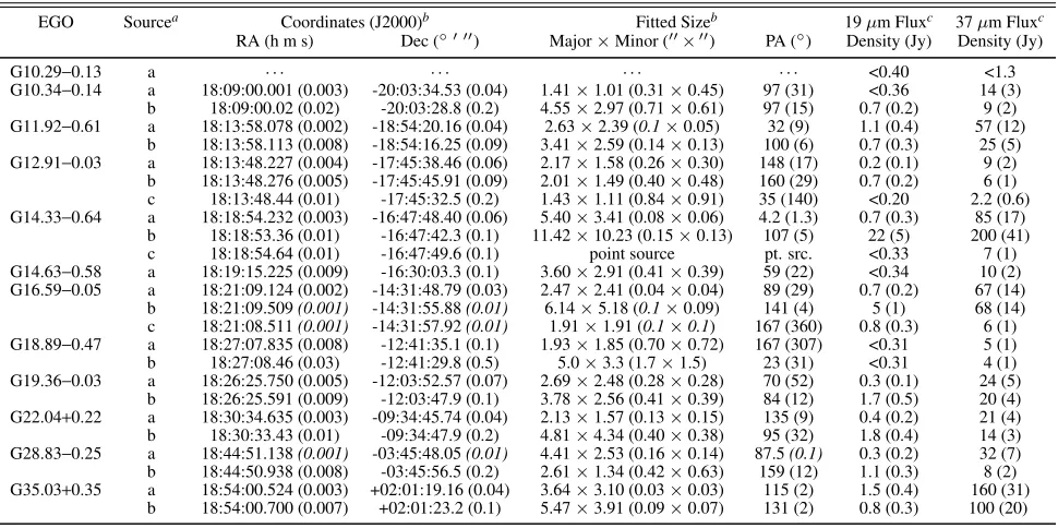
SOFIA FORCAST 19.7µM AND37.1µMFITTEDFLUXDENSITIES

EGO Sourcea _{Coordinates (J2000)}b _{Fitted Size}b _{19µm Flux}c _{37µm Flux}c

RA (h m s) Dec (◦ 0 00) Major×Minor (00×00_{) PA (}◦_{) Density (Jy) Density (Jy)}

G10.29−0.13 a · · · <0.40 <1.3

G10.34−0.14 a 18:09:00.001 (0.003) -20:03:34.53 (0.04) 1.41×1.01 (0.31×0.45) 97 (31) <0.36 14 (3) b 18:09:00.02 (0.02) -20:03:28.8 (0.2) 4.55×2.97 (0.71×0.61) 97 (15) 0.7 (0.2) 9 (2) G11.92−0.61 a 18:13:58.078 (0.002) -18:54:20.16 (0.04) 2.63×2.39 (0.1×0.05) 32 (9) 1.1 (0.4) 57 (12)

b 18:13:58.113 (0.008) -18:54:16.25 (0.09) 3.41×2.59 (0.14×0.13) 100 (6) 0.7 (0.3) 25 (5) G12.91−0.03 a 18:13:48.227 (0.004) -17:45:38.46 (0.06) 2.17×1.58 (0.26×0.30) 148 (17) 0.2 (0.1) 9 (2)

b 18:13:48.276 (0.005) -17:45:45.91 (0.09) 2.01×1.49 (0.40×0.48) 160 (29) 0.7 (0.2) 6 (1) c 18:13:48.44 (0.01) -17:45:32.5 (0.2) 1.43×1.11 (0.84×0.91) 35 (140) <0.20 2.2 (0.6) G14.33−0.64 a 18:18:54.232 (0.003) -16:47:48.40 (0.06) 5.40×3.41 (0.08×0.06) 4.2 (1.3) 0.7 (0.3) 85 (17)

b 18:18:53.36 (0.01) -16:47:42.3 (0.1) 11.42×10.23 (0.15×0.13) 107 (5) 22 (5) 200 (41) c 18:18:54.64 (0.01) -16:47:49.6 (0.1) point source pt. src. <0.33 7 (1) G14.63−0.58 a 18:19:15.225 (0.009) -16:30:03.3 (0.1) 3.60×2.91 (0.41×0.39) 59 (22) <0.34 10 (2) G16.59−0.05 a 18:21:09.124 (0.002) -14:31:48.79 (0.03) 2.47×2.41 (0.04×0.04) 89 (29) 0.7 (0.2) 67 (14)

b 18:21:09.509(0.001) -14:31:55.88(0.01) 6.14×5.18 (0.1×0.09) 141 (4) 5 (1) 68 (14) c 18:21:08.511(0.001) -14:31:57.92(0.01) 1.91×1.91 (0.1×0.1) 167 (360) 0.8 (0.3) 6 (1) G18.89−0.47 a 18:27:07.835 (0.008) -12:41:35.1 (0.1) 1.93×1.85 (0.70×0.72) 167 (307) <0.31 5 (1) b 18:27:08.46 (0.03) -12:41:29.8 (0.5) 5.0×3.3 (1.7×1.5) 23 (31) <0.31 4 (1) G19.36−0.03 a 18:26:25.750 (0.005) -12:03:52.57 (0.07) 2.69×2.48 (0.28×0.28) 70 (52) 0.3 (0.1) 24 (5)

b 18:26:25.591 (0.009) -12:03:47.9 (0.1) 3.78×2.56 (0.41×0.39) 84 (12) 1.7 (0.5) 20 (4) G22.04+0.22 a 18:30:34.635 (0.003) -09:34:45.74 (0.04) 2.13×1.57 (0.13×0.15) 135 (9) 0.4 (0.2) 21 (4) b 18:30:33.43 (0.01) -09:34:47.9 (0.2) 4.81×4.34 (0.40×0.38) 95 (32) 1.8 (0.4) 14 (3) G28.83−0.25 a 18:44:51.138(0.001) -03:45:48.05(0.01) 4.41×2.53 (0.16×0.14) 87.5(0.1) 0.3 (0.2) 32 (7) b 18:44:50.938 (0.008) -03:45:56.5 (0.2) 2.61×1.34 (0.42×0.63) 159 (12) 1.1 (0.3) 8 (2) G35.03+0.35 a 18:54:00.524 (0.003) +02:01:19.16 (0.04) 3.64×3.10 (0.03×0.03) 115 (2) 1.5 (0.4) 160 (31)

b 18:54:00.700 (0.007) +02:01:23.2 (0.1) 5.47×3.91 (0.09×0.07) 131 (2) 0.8 (0.3) 100 (20) a_{The listed source positions and fitted sizes are from the 37.1µm fit results only.}

b_{G10.29−0.13 has “· · ·” in place of coordinates and fitted size because it was a non-detection at both wavelengths.}

c_{Upper limits are given for sources that have no emission above 5σ. In these cases, the listed upper limit is the 5σvalue for the FOV.}

respectively) using CASAViewer. However, because the flux in these bands likely includes emission from some sources or processes unrelated to our sources of interest, and because the SED models we employ in § 4.2 do not include emission from PAHs, we chose to include these data as upper limits.

We obtained the necessary IRAC images from the NASA/IPAC Gator Catalog List, and aperture corrections were applied to each measurement according to the table on

page 27 of the IRAC Instrument Handbook10_{. We did not}

include measurements in the 4.5µm (I2) band because the

emission in this band is extended in all cases (this was the original classification criterion for this object type).

The background noise level for the IRAC bands, as for all other wavelengths, is the scaled MAD within an emission-free region in each image. The emission-emission-free regions were identical for all three IRAC bands used. For each source with significant (>5σ) emission at 37.1µm, we measured the inte-grated IRAC band flux within a circular aperture centered on

the 37.1µm coordinates. We also measured the flux within

an annulus of corresponding size. Aperture and annulus sizes were chosen based on the aperture corrections listed in the IRAC Instrument Handbook and the FWHM of each source in each band. For a given source, we used the same aperture for all three IRAC bands (i.e. we did not modify the size of the aperture with wavelength); we chose the smallest aperture that would successfully fit a source in all three bands. Each inte-grated flux measurement was corrected for background emis-sion by subtracting the product of the median intensity value within the annulus and the size of the aperture from the direct aperture-flux measurement. After this subtraction, we applied the appropriate aperture corrections as listed in the IRAC In-strument Handbook. All aperture and annulus radii, aperture

10_{https://irsa.ipac.caltech.edu/data/SPITZER/docs/irac/iracinstrumenthandbook/}

corrections, and corrected fluxes for our sources are listed in Table 4.

Due to the very crowded nature of these fields in the IRAC bands and the generally clustered nature of our sources, it was sometimes necessary to use annuli for local background subraction that were not centered on our sources. When this was necessary, we chose isolated stars within the same field of view and centered our annuli on those sources. We were careful to choose annulus stars of similar or lower bright-ness than the source in question. Choosing a star of equal or lower brightness for background subtraction would only

have the effect ofincreasingthe measured flux density. While

it does sacrifice some precision, allowing the measured flux density to perhaps be artificially increased maintains the self-consistency of the photometry, as the data from these bands will only be used as upper limits.

The uncertainties on the integrated flux densities are the quadrature sum of three values: the background noise lev-els, the absolute flux calibration uncertainty for the IRAC bands, and the uncertainty in the aperture-correction values. The background noise levels are discussed above. The IRAC Instrument Handbook quotes an absolute flux calibration ac-curacy to within 3% of the total integrated flux for a given object, and that is the value we adopt here. Additionally, the Handbook quotes an absolute aperture-correction accuracy to within 2% of the total aperture-correction factor.

3.2.2. Spitzer MIPS Photometry

We used CASA’simfittask to determine the integrated

flux densities of our targets at 24µm using the same fitting

procedure described in § 3.1. Due to the MIPS 24µm

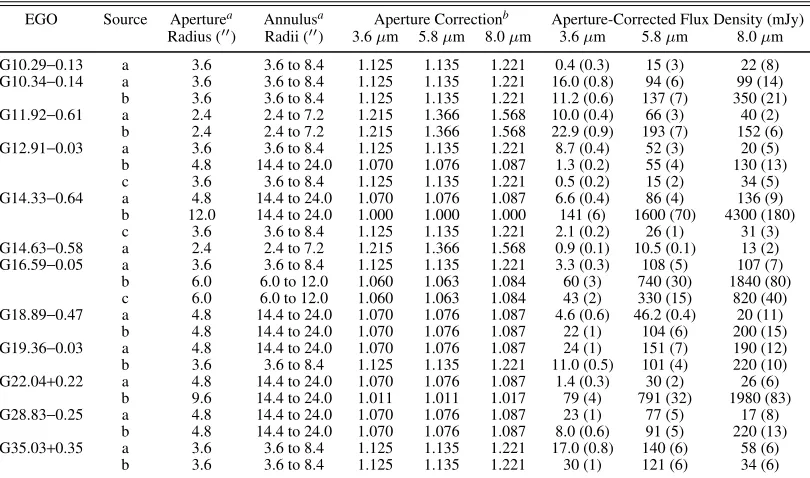
Hand-TABLE 4

IRAC INTEGRATEDFLUXDENSITIES

EGO Source Aperturea _Annulusa _{Aperture Correction}b _{Aperture-Corrected Flux Density (mJy)}

Radius (00) Radii (00) 3.6µm 5.8µm 8.0µm 3.6µm 5.8µm 8.0µm G10.29−0.13 a 3.6 3.6 to 8.4 1.125 1.135 1.221 0.4 (0.3) 15 (3) 22 (8) G10.34−0.14 a 3.6 3.6 to 8.4 1.125 1.135 1.221 16.0 (0.8) 94 (6) 99 (14)

b 3.6 3.6 to 8.4 1.125 1.135 1.221 11.2 (0.6) 137 (7) 350 (21) G11.92−0.61 a 2.4 2.4 to 7.2 1.215 1.366 1.568 10.0 (0.4) 66 (3) 40 (2)

b 2.4 2.4 to 7.2 1.215 1.366 1.568 22.9 (0.9) 193 (7) 152 (6) G12.91−0.03 a 3.6 3.6 to 8.4 1.125 1.135 1.221 8.7 (0.4) 52 (3) 20 (5)

b 4.8 14.4 to 24.0 1.070 1.076 1.087 1.3 (0.2) 55 (4) 130 (13) c 3.6 3.6 to 8.4 1.125 1.135 1.221 0.5 (0.2) 15 (2) 34 (5) G14.33−0.64 a 4.8 14.4 to 24.0 1.070 1.076 1.087 6.6 (0.4) 86 (4) 136 (9)

b 12.0 14.4 to 24.0 1.000 1.000 1.000 141 (6) 1600 (70) 4300 (180) c 3.6 3.6 to 8.4 1.125 1.135 1.221 2.1 (0.2) 26 (1) 31 (3) G14.63−0.58 a 2.4 2.4 to 7.2 1.215 1.366 1.568 0.9 (0.1) 10.5 (0.1) 13 (2) G16.59−0.05 a 3.6 3.6 to 8.4 1.125 1.135 1.221 3.3 (0.3) 108 (5) 107 (7)

b 6.0 6.0 to 12.0 1.060 1.063 1.084 60 (3) 740 (30) 1840 (80) c 6.0 6.0 to 12.0 1.060 1.063 1.084 43 (2) 330 (15) 820 (40) G18.89−0.47 a 4.8 14.4 to 24.0 1.070 1.076 1.087 4.6 (0.6) 46.2 (0.4) 20 (11)

b 4.8 14.4 to 24.0 1.070 1.076 1.087 22 (1) 104 (6) 200 (15) G19.36−0.03 a 4.8 14.4 to 24.0 1.070 1.076 1.087 24 (1) 151 (7) 190 (12) b 3.6 3.6 to 8.4 1.125 1.135 1.221 11.0 (0.5) 101 (4) 220 (10) G22.04+0.22 a 4.8 14.4 to 24.0 1.070 1.076 1.087 1.4 (0.3) 30 (2) 26 (6)

b 9.6 14.4 to 24.0 1.011 1.011 1.017 79 (4) 791 (32) 1980 (83) G28.83−0.25 a 4.8 14.4 to 24.0 1.070 1.076 1.087 23 (1) 77 (5) 17 (8)

b 4.8 14.4 to 24.0 1.070 1.076 1.087 8.0 (0.6) 91 (5) 220 (13) G35.03+0.35 a 3.6 3.6 to 8.4 1.125 1.135 1.221 17.0 (0.8) 140 (6) 58 (6)

b 3.6 3.6 to 8.4 1.125 1.135 1.221 30 (1) 121 (6) 34 (6) a_{These columns list the radii of the aperture and annuli used for aperture photometry for each source. Radii are listed in arcseconds. Pixel scale is}

1.002/pixel for all IRAC bands.

b_{Aperture correction factors are from the IRAC Instrument Handbook.}

book11), the MIPS fit results require an aperture correction

similar to that discussed in § 3.1. Fortunately, the MIPS im-ages, unlike our SOFIA imim-ages, contain a plethora of isolated point sources with which to measure the PSF directly.

In order to determine the value of the necessary aperture

correction, we performed the imfit fitting procedure

de-scribed in § 3.1 on five isolated, relatively bright point sources with fluxes listed in the MIPSGAL Point Source Catalog (Gutermuth & Heyer 2015). We selected the sources to span a

range of colors and 24µm flux densities. As with the SOFIA

sources, we considered fits to be “satisfactory” when the ab-solute value of the residuals within the Airy disk were all

un-der 4×MAD of the residual image, with the majority under

2×MAD. We compared the integrated fluxes returned by the

imfit task to those listed in the MIPSGAL Point Source Catalog. We found a consistent aperture correction value of

1.59±0.00893. Table 5 shows the positions, catalog fluxes,

fitted flux results, and calculated flux ratios for these five stan-dard stars.

We then applied the fitting procedure and measured

aper-ture correction to our science targets. As for the SOFIA

FORCASTdata, sometimes certain parameters (source

posi-tion, size, etc.) were held fixed during the fitting procedure; these cases are noted in Table 6. Our results are listed in Ta-ble 6, which presents the final, aperture-corrected fitted flux results (to be used in the SED fitting) as well as the initial,

un-correctedimfitflux results.

As with the SOFIA data, the uncertainties on the integrated flux density values are the quadrature sum of the uncertainties

returned by theimfittask, the uncertainty of our calculated

aperture-correction value, and the absolute flux calibration uncertainty for the MIPS data. The MIPS Instrument

Hand-11_{http://irsa.ipac.caltech.edu/data/SPITZER/docs/mips/mipsinstrumenthandbook/}

book quotes an absolute flux calibration accuracy to within 5% of the total integrated flux of a given object. The uncer-tainties on both the peak intensity and the integrated flux

den-sity returned byimfitare set by the background noise level,

which we set to the scaled MAD during the fitting procedure. The uncertainty of the calculated aperture correction value we take to be the standard deviation of the five measured values: 8.93×10−3_.

3.2.3. Hi-GAL and ATLASGAL Photometry

Unlike with the near- and mid-infrared data sets, our far-IR data could rarely be considered point-like. Therefore,

in-stead of fitting gaussians to the emission using imfit, we

measured the integrated flux of each source within a given in-tensity level using CASAViewer. The inin-tensity levels were chosen uniquely for each source depending on local

back-ground emission and the overall image noise level (σ).

Gener-ally, apertures for the ATLASGAL data followed the 5σlevel.

Apertures for the Hi-GAL data varied between 60σand 200σ

at 70µm and between 40σand 150σat 160µm. These

aper-tures follow comparatively high contours due to the

combina-tion of low scaledMADvalues (typically of order 10−1) and,

in most cases, relatively bright large-scale ambient emission. Each integrated flux measurement was corrected for this back-ground emission by subtracting the product of the median in-tensity value within a local annulus and the size of the aper-ture from the direct aperaper-ture-flux measurement. The mean and median aperture radii at 70 µm are 19.006 and 18.008,

re-spectively, as compared to the HiGAL 70µm beam size of

5.008×12.001. The mean and median aperture radii at 160µm are 26.00_{3 and 26.}00_{7, respectively, as compared to the HiGAL}

TABLE 5

MIPS 24µMSTANDARDSTARFITTED ANDCATALOGFLUXES, & FLUX

RATIOS

Stara Coordinates (J2000)b Catalog Flux Fitted Flux Flux Ratio RA (h m s) Dec (◦ 0 00) (mJy) (mJy)

1 18:30:32.40 -09:35:47.25 1950 (39) 1220 (40) 1.60 2 18:30:12.78 -09:36:47.99 1980 (36) 1250 (38) 1.58 3 18:30:53.95 -09:39:51.27 2960 (55) 1870 (71) 1.58 4 18:30:46.32 -09:32:28.89 1230 (23) 770 (23) 1.60 5 18:30:48.45 -09:36:00.11 780 (14) 490 (17) 1.59 a_{Coordinates and both fitted (this work) and catalog (Gutermuth & Heyer 2015) flux densities}

for five bright, isolated point sources in the MIPSGAL Point Source Catalog.

b_{Listed coordinates are from the MIPS Point Source Catalog (Gutermuth & Heyer 2015).}

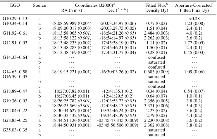
TABLE 6

MIPS 24µMAPERTURE-CORRECTEDFITTEDFLUXDENSITIES

EGO Source Coordinates (J2000)a _{Fitted Flux}b _{Aperture-Corrected}c

RA (h m s) Dec (◦ 0 00) Density (Jy) Fitted Flux (Jy)

G10.29−0.13 a · · · <0.28

G10.34−0.14 a 18:08:59.989 (0.004) -20:03:34.97 (0.06) 0.77 (0.03) 1.23 (0.08) b 18:09:00.017 (0.003) -20:03:28.75 (0.05) 1.51 (0.04) 2.4 (0.1) G11.92−0.61 a 18:13:58.065(0.001) -18:54:21.26(0.01) 2.484 (0.003) 4.0 (0.2) b 18:13:58.122(0.001) -18:54:14.97(0.01) 2.262 (0.003) 3.6 (0.2) G12.91−0.03 a 18:13:48.233 (0.002) -17:45:38.19 (0.03) 1.11 (0.02) 1.77 (0.09)

b 18:13:48.283 (0.001) -17:45:46.21 (0.01) 1.50 (0.01) 2.4 (0.1) c 18:13:48.469 (0.004) -17:45:31.77 (0.04) 0.28 (0.01) 0.45 (0.03)

G14.33−0.64 a · · · confused · · ·

b · · · saturated · · ·

c · · · confused · · ·

G14.63−0.58 a 18:19:15.221 (0.001) -16:30:03.26 (0.02) 0.683 (0.009) 1.09 (0.06)

G16.59−0.05 a · · · saturated · · ·

b · · · saturated · · ·

c · · · confused · · ·

G18.89−0.47 a 18:27:07.82 (0.01) -12:41:35.1 (0.2) 0.34 (0.04) 0.54 (0.07)

b 18:27:08.45 (0.01) -12:41:29.5 (0.2) 0.64 (0.07) 1.0 (0.1) G19.36−0.03 a 18:26:25.782(0.001) -12:03:53.73(0.01) 2.356 (0.005) 3.8 (0.2) b 18:26:25.569(0.001) -12:03:48.13(0.01) 3.371 (0.006) 5.4 (0.3) G22.04+0.22 a 18:30:34.627 (0.001) -09:34:46.24 (0.02) 2.23 (0.02) 3.6 (0.2) b 18:30:33.432(0.001) -09:34:48.39(0.01) 2.79 (0.02) 4.4 (0.2) G28.83−0.25 a 18:44:51.136 (0.001) -03:45:47.845 (0.009) 2.230 (0.008) 3.6 (0.2) b 18:44:50.931 (0.001) -03:45:56.506 (0.009) 2.362 (0.008) 3.8 (0.2)

G35.03+0.35 a · · · saturated · · ·

b · · · saturated · · ·

a_{Source coordinates are the fitted coordinates returned byimfit. Sources that have · · · values in place of coordinate values are}

either undetected at 24µm (G10.29−0.13) or suffer from saturation and/or confusion (G14.33−0.64, G16.59−0.05, G35.03+0.35). Sources with position uncertainties in italics (G11.92−0.61, G19.36−0.03, G22.04+0.22_b) had their coordinates held fixed during the fitting procedure, so the position uncertainties come not from theimfitresults but from the uncertainty in the choice of source position (usually of order 0.01 pixels, or, 0.000125).

b_{These are the fitted fluxes directly returned byimfit; they have not been corrected for aperture effects. Sources with “ · · · ”}

are nondetections at 24µm. Sources listed as “saturated” are saturated at 24µm. Sources listed as “confused” are not saturated at 24µm but suffer from an angular confusion problem, usually with a nearby saturated source.

c_{These are the aperture-corrected fitted flux densities, where the applied aperture correction is 1.59±0.00893, as calculated in}

Table 5. We use the data in this column for constructing our SEDs. Sources listed as “ · · · ” could not be fit at 24µm due to saturation and/or confusion issues and thus have no fitted flux value to which to apply an aperture correction.

Our far-IR flux uncertainties are the quadrature sum of two values. First, there is the statistical uncertainty of the mea-surement itself, which we take to be the product of the

back-ground noise levelσin Jy beam−1_{and the square root of the}

aperture size in beams. Second, there is the inherent uncer-tainty of the image due to flux calibration accuracy. Moli-nari et al. (2016) quote an absolute flux uncertainty of 5% for the Hi-GAL data, and Schuller et al. (2009) quote an absolute flux uncertainty of 15% for the ATLASGAL survey. We adopt these values for our uncertainty calculations for the Hi-GAL and ATLASGAL data, respectively.

Far-IR source selection— Beginning at 70µm, the fluxes of

sources that are not dominant at 37.1 µm (sources “b” and

“c” for each FOV) begin to decrease, in some cases rapidly.

This decrease in flux is usually such that, by either 160µm or

870µm, there is only one dominant source at that wavelength.

In all cases, that dominant source is spatially coincident with

the location of the brightest source at 37.1µm. However, the

EGO, but neither is it clear that the spatial coincidence is not merely a result of resolution limitations. In cases where the

morphology of the 70µm or 160 µm emission was

consis-tent with a single source, we assigned all the emission in that band to source “a.” In cases where it was clear that there were multiple sources present in the Hi-GAL data, we took one of two approaches. First, we attempted to fit the

emis-sion using multiple gaussian components usingimfit. If we

achieved satisfactory fits with this approach, the fitted fluxes of both sources are listed in Table 7. Second, if we could not achieve satisfactory fits with multiple gaussian components, we attempted to estimate the maximum possible amount of flux that could be ascribed to the weaker source. We then performed the photometric procedure described above on the emission as a whole (dominant and weaker source combined)

and assigned all of the resulting flux to the dominant 37.1µm

source, and added the estimated flux from the weaker source to our uncertainty value for the dominant source. For these cases, the measured fluxes are marked in bold in Table 7. While imperfect, this method does allow us to at least ac-count for the effects of multiple blended sources even when we cannot satisfactorily deblend the emission itself.

Source confusion was not an issue in any of the ATLAS-GAL images, since the ATLASATLAS-GAL data a) have an angu-lar resolution that is significantly poorer than any of the other data sets, thus potentially blending any individual sources past the point where one could recognize separate sources, and b) necessarily probe cooler gas. This effectively means that the emission in the ATLASGAL images originates primarily in the outer regions of the parent clump, which is an identifiably larger physical size scale than those probed by the Hi-GAL and our mid- or near-IR data sets. Due to source morphol-ogy in the ATLASGAL data and the aforementioned drop in flux in the FIR for sources that are not the dominant source at

37.1µm, we attribute all 870µm flux to the single, dominant

37.1µm source in all cases.

The effect of these source-selection criteria is that full SEDs

are constructed for the brightest 37.1 µm sources (the “a”

sources) only, and these SEDS are based on the explicit as-sumption that these sources are by far the most dominant in the far-IR.

3.3. Images and Trends

Figures 1 through 4 show the detected SOFIA 19.7 and

37.1µm emission in the vicinity of each EGO. We detected

37.1 µm emission in all twelve fields; in eleven cases, this

emission was associated with the EGO. This is in itself a high detection rate. However, we detect an average of only two sources per target, of which only one, on average, is actu-ally associated with the EGO. This suggests that, rather than detecting multiple protostars within each protocluster, we are typically detecting only the dominant source in each EGO.

Likewise, we detect 19.7µm emission in nine of our twelve

fields, but it is only associated with the target EGO in eight

cases. We detect more 19.7µm emission toward sources that

are not associated with the target EGOs than emission toward sources that are (10/18 not associated versus 8/18 that are).

At 19.7 µm, we still detect an average of two sources per

target. Taken together, these trends suggest that our target protoclusters are still quite young and/or deeply-embedded; this would explain the trend of overall dominance by a sin-gle source, as well as the poorer detection rate of even these

dominant sources at 19.7µm.

Of our 37.1µm sources, all but one are located entirely

within the 25% ATLASGAL contours of the clump associated

with the target EGO, for a total of 23 37.1µm sources within

eleven ATLASGAL clumps (G10.29−0.13 has no 37.1 µm

emission toward the EGO itself, so its ATLASGAL clump is not counted). This is an average of slightly more than two

mid-infrared sources per clump. The one 37.1 µm source

not located within an ATLASGAL clump is G14.33−0.64_b,

which has some extended emission within the 870 µm

con-tours but is centered outside of it; our source G14.33−0.64_b

is the known HIIregion IRAS 18159−1648 (Jaffe et al. 1982).

Eleven of our sources are located in IRDCs; the only ex-ception is G16.59−0.05. Eleven sources are known to be

co-incident with 6.7 GHz CH3OH masers (references for maser

detections are in the tablenotes of Table 1); the remain-ing source, G14.33−0.64, has no published 6.7 GHz data at the time of writing. Three sources - G10.29−0.13 and

G10.34−0.14 (near the W31 HII region G10.32−00.15, see

Westerhout 1958), and G28.83−0.25 (near N49, see Wink et

al. 1982) - are adjacent to are known HIIor UCHIIregions.

3.4. Mid-infrared Multiplicity

There is some evidence of multiplicity at mid-infrared wavelengths for nearly all of our targets, with G10.29−0.13 (lacking any mid-IR detection) and G14.63−0.58 being the only exceptions. The evidence for mid-IR multiplicity for the other sources falls generally into two categories: individual EGO-related sources (i.e. within the boundaries of extended

4.5µm emission) that have unresolved substructure at the

an-gular resolution of our SOFIA data, and sources that have

nearby (_.1000) 37.1µm detections which are not within the

extended 4.5um emission of the EGO, and whose association with the EGO is unclear. We discuss each category in greater detail in the following sections. The naming convention of the new detections is described in § 3.1.

3.4.1. EGO Sources with Unresolved Substructure at 37.1µm

The dominant EGO-related sources in G11.92−0.61, G14.33−0.58, G28.83−0.25, G35.03+0.35 exhibit elongated,

unresolved 37.1 µm emission suggestive of multiplicity at

scales_.500(the SOFIA angular resolution is 3.004). Below we explore how the mid-IR emission compares to existing high resolution centimeter to millimeter data. This comparison helps inform the nature of the emission at each wavelength. Mid-IR emission may trace both hot cores and outflow cavi-ties, while centimeter emission can trace both free-free

emis-sion (e.g. HII region, ionized jet) and the long-wavelength

end of the Rayleigh-Jeans tail of dust emission. Millimeter observations (in this context) primarily serve to identify indi-vidual cores from dust continuum emission. By comparing the emission from these different wavelength regimes, we can attempt to disentangle the possible sources of mid-IR emis-sion in these objects.

G11.92−0.61— G11.92−0.61 is elongated roughly N-S at

37.1 µm, and shows two distinct sources at 19.7µm which

lie along the axis of the 37.1 µm elongation (Fig. 1). The

southern and northern mid-IR sources (G11.92−0.61_a and G11.92−0.61_b) are coincident with the (sub)millimeter pro-tostellar sources MM1 and MM3, respectively (Cyganowski et al. 2011a, 2017). Both MM1 and MM3 are associated

with 6.7 GHz CH3OH masers (a signpost of massive star

TABLE 7

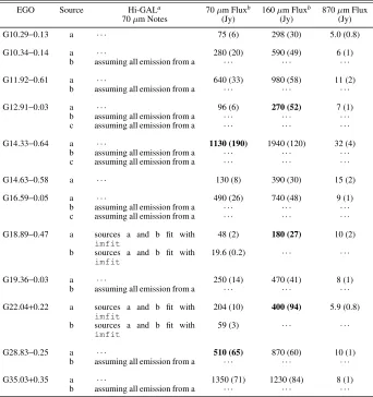
HI-GAL 70µM& 160µM ANDATLASGAL 870µMFLUXDENSITIES

EGO Source Hi-GALa _{70µm Flux}b _{160µm Flux}b _{870µm Flux}

70µm Notes (Jy) (Jy) (Jy)

G10.29−0.13 a · · · 75 (6) 298 (30) 5.0 (0.8)

G10.34−0.14 a · · · 280 (20) 590 (49) 6 (1)

b assuming all emission from a · · · ·

G11.92−0.61 a · · · 640 (33) 980 (58) 11 (2)

b assuming all emission from a · · · ·

G12.91−0.03 a · · · 96 (6) 270 (52) 7 (1)

b assuming all emission from a · · · ·

c assuming all emission from a · · · ·

G14.33−0.64 a · · · 1130 (190) 1940 (120) 32 (4)

b assuming all emission from a · · · ·

c assuming all emission from a · · · ·

G14.63−0.58 a · · · 130 (8) 390 (30) 15 (2)

G16.59−0.05 a · · · 490 (26) 740 (48) 9 (1)

b assuming all emission from a · · · ·

c assuming all emission from a · · · ·

G18.89−0.47 a sources a and b fit with

imfit

48 (2) 180 (27) 10 (2) b sources a and b fit with

imfit

19.6 (0.2) · · · ·

G19.36−0.03 a · · · 250 (14) 470 (41) 8 (1)

b assuming all emission from a · · · ·

G22.04+0.22 a sources a and b fit with

imfit

204 (10) 400 (94) 5.9 (0.8) b sources a and b fit with

imfit

59 (3) · · · ·

G28.83−0.25 a · · · 510 (65) 870 (60) 10 (1)

b assuming all emission from a · · · ·

G35.03+0.35 a · · · 1350 (71) 1230 (84) 8 (1)

b assuming all emission from a · · · ·

a_{This column addresses the confusion of our sources at the 70µm wavelength and angular resolution. Sources with the}

note “assuming all emission from a” do have 70µm emission coincident with the position of source b and/or c, but we assume the emission to be entirely from or significantly dominated by source a. Sources with the note “sources a and b fit withimfit” have emission coincident with both source a and source b, and there were two emission regions sufficiently distinguishable at 70µm to be fit with theimfittool. These notes only apply to the 70µm data.

b_{The sources inboldin these two columns suffer from confusion at either 70 or 160µm, and were not sufficiently}

well-separated to be successfully fit with two componentsimfit. In these cases, the uncertainties of the flux densities are increased to reflect this effect. The precise method by which the uncertainties account for the confusion issue is discussed in detail in-text in § 3.2.3.

2011b; Cyganowski et al. 2014; Moscadelli et al. 2016; Ilee et al. 2016; Towner et al. 2017).

To further explore how sensitive the SOFIA data are to the presence of multiple protostellar sources, we turn to high-angular resolution, high-sensitivity millimeter data. Atacama Large Millimeter/submillimeter Array (ALMA) observations

of G11.92−0.61 (1.05 mm, 0.0049×0.0034 synthesized beam)

by Cyganowski et al. (2017) reveal at least eight 1.05 mm

sources within a 500radius of the peak of the 37.1µm

emis-sion, two of which correspond to MM1 and MM3). Of these eight, the authors estimate that six are low-mass objects, one is intermediate- or high-mass (MM3), and one is high-mass (MM1). Indeed, follow-up observations of MM1 at 1.3 mm

using ALMA, with a synthesized beam of 0.00106 ×0.00079,

find that this source is likely a proto-O star whose

circum-stellar disk dynamics yield an enclosed mass of Menc∼40±

5M(Ilee et al. 2018). These radio data suggest that the

mid-IR morphology of G11.92−0.61 is dominated by the two in-termediate to massive protostellar sources (MM1 and MM3), rather than, e.g., a poorly-resolved outflow cavity. This result also indicates that our SOFIA data are sensitive to massive protostellar multiplicity, though as expected the mid-IR data are not sensitive to lower mass (and luminosity) protocluster members (also see § 4.3.1).

G14.33−0.64— The dominant EGO-related source G14.33−0.64_a (Fig. 2) is slightly elongated N-S at

37.1µm, and there is a 19.7µm detection associated with the

northern portion of the elongation. The brightest component,

G14.33−0.64_b, is coincident with the known evolved HII

region IRAS 18159−1648. In order to achieve satisfactory

fits to the 37.1 µm emission toward G14.33−0.64_a, it is

necessary to fit a third component. G14.33−0.64_c is located

∼ 400 east-southeast of G14.33−0.64_a, is faint at both