All Pairs Shortest Path Algorithms

(1)

All Pairs Shortest Path Algorithms

5th November 1999 16:01

(2)

Abstract

There are many algorithms for the all pairs shortest path problem, depending on variations of the problem. The simplest version takes only the size of vertex set as a parameter. As additional parameters, other problems specify the number of edges and/ or the maximum value of edge costs.

(3)

Chapter 1 Introduction

This report presents the reader with a new approach to solving the all pairs shortest path problem. This approach involves looking at the structure of the graph and then using this information to help decrease the time complexity of the problem.

As discussed in section 2.1 a number of approaches have already been taken that take into consideration the structure of the graph, yet none of these have ever looked at the values that make up the distance matrix.

The structure of this report is as follows, in the second chapter a brief intro-duction to what the all pairs shortest path problem is given, along with its re-lationship to distance matrix multiplication. The rere-lationship between distance matrix multiplication and arithmetic matrix multiplication is also discussed in this chapter.

In the third chapter three algorithms are discussed that the author has im-plemented during the year. A small decrease in the time complexity of the third algorithm was found.

Chapter four expands on the work done in the previous chapter. It develops the idea of spectral theory and then further refines this into an algorithm for performing distance matrix multiplication. At the end of this chapter a problem with the spectral theory algorithm is discussed that prevents it from being used to solve the all pairs shortest path problem.

In chapter five another algorithm is presented that modifies the algorithm from chapter four. This new algorithm is then able to calculate the all pairs shortest path problem for graphs that have a specific structure.

Chapter six of this report offers the reader an example of an application area where the all pairs shortest path problem could be used .. The maximum sub-array problem was recently found to be equivalent to the all pairs shortest path problem and as such could benefit from any decrease in the time complexity of the all pairs shortest path algorithms.

Chapter seven presents something completely different from what the other chapters were presenting. In this chapter a brief look at a graphical user interface tool for displaying running all pairs shortest path algorithms is presented.

(5)

Chapter

2 All Pairs Shortest Path

Algorithm

2.1 Work Previously Done

Over the years there has been a large amount of work done in the field of the all pairs shortest path problem. This work has seen people conclude that the all pairs shortest path is the same as distance matrix multiplication[l

J.

Authors have discovered new upper bounds on the time complexity of the problem [2]. Algorithms that deal with nearly acyclic directed graphs have been found (3]. Finally algorithms with expected running time of 0( n2log n) have been found[4]. No work has been done on actually looking at the values that make up the distance matrix.

2.2 All Pairs Shortest Path Problem

The all pairs shortest path problem involves finding the shortest path from each node in the graph to every other node in the graph. A directed graph is presented in Figure 2.1. This can be calculated by using a number of different algorithms. One way is simply to perform a single source algorithm, this problem calculates the shortest path from one node to every other node, and applies it to all the nodes in the graph.

Another way is to present the graph as a matrix, this can be seen in Fig-ure 2.1 which shows a graph. The corresponding matrix representation of the graph is given in Figure 2.2. Once this matrix has been constructed, distance matrix multiplication can be performed on it, distance matrix multiplication is explained in section 2.3. The method of repeated squaring is used on the matrix log n times. Once this repeated squaring has been completed the matrix will then contain the solution to the all pairs shortest path problem.

(6)

[image:6.595.113.387.115.398.2]

All Pairs Shortest Path

Figure 2.1: A directed graph 0

_-

10 18

6 0

-

4

-

2 0

--

1 0

Figure 2.2: The matrix for the graph from figure 2.1

2.3 Distance Matrix Multiplication

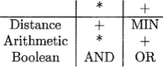
Distance matrix multiplication is similar to matrix multiplication except where multiplication is used addition is used and where addition is used the min oper-ator is used. This operoper-ator selects the minimum number from a set of numbers. The above information is presented in the table shown in Figure 2.3. Also presented in the table is boolean matrix multiplication.

Distance matrix multiplication has the same time complexity as matrix mul-tiplication, and as such algorithms for both of them can easily be adapted to perform either matrix multiplication or distance matrix multiplication. The simplest algorithm for performing matrix multiplication is set out in Figure 2.4. This algorithm must perform line 4 n3 _{times and as such has time complexity}

of O(n3 ).

This simple algorithm for matrix multiplication can easily be shown to have O(n3₎_{time complexity. This simple matrix multiplication algoritlun can easily}

*

Distance

+

Arithmetic

*

Boolean AND

+

MIN

+

[image:6.595.221.340.644.693.2]

OR

(7)

Takaoka and Cook

0 Initialise Matrix; 1 for(i=O;i<n;i++) { 2 for(j=O;j<n;j++) { 3 for(l=O;l<n;l++) {

4 Matrix[i] [j] += Matrix[i] [1]

*

Matrix[l] [j];

Figme 2.4: Simple program code to perform matrix multiplication

0 Initialise Matrix; 1 for(i=O;i<n;i++) 2 for(j=O;j<n;j++) 3 for(k=O;l<n;l++)

4 if(Matrix[i] [k] > Matrix[i] [j] + Matrix(j] [i]) 5 Matrix[i] [k] = Matrix[i] [j] + Matrix[j][i];

Figure 2.5: Floyd's all pairs shortest path algorithm

be adapted to the distance matrix multiplication algorithm.

2.4 Basic All Pairs Shortest Path Algorithms

There exists some basic algorithms for solving the all pairs shortest path prob-lem. Two examples of these are Floyd's[5] see Figure 2.5, and repeated squaring of the distance matrix see Figme 2.7. These algorithms have time complexity of O(n3₎_{and O(n}3₎_{log n.}_{The basic code for both of these algorithms is set} out in the two figures.

By using Floyd's algorithm, presented in Figme 2.5, on the graph from Figure 2.1 a solution matrix is given in Figure 2.6.

0 12

6 0

8 2

9 3

10 18 5 4

0 6

1 0

(8)

0 Initialise Matrix; 1 for(k=O;k<(log(n));k++) 2 for(i=O;i<n;i++) 3 for(j=O;j<n;j++) 4 for(l=O;l<n;l++)

All Pairs Shortest Path Algorithms

5 i f (Matrix [i] [j] > Matrix [i] [l] + Matrix [l] [j])

Matrix [i] [j] = Matrix [i] [l] + Matrix [l] [j] ;

(9)

Chapter 3 Implementation of 3 All

Pairs Shortest Path

Algorithms

Presented in this chapter are three algorithms that at the start of year the author was looking at. From the third of these algorithm's, the new algorithms pre..<>ented in chapter four and chapter five were found. These algorithms can be found in a paper presented by T. Takaoka[6].

These algorithms are based on to distinct phases an accelerating phase and a cruising phase. Both these phases are combined to solve the problem. The accelerating phase uses a previously written algorithm and stops this algorithm at a particular point called r. Then it switches to the cruising phase, which is used to finish calculating the solution. This is summarised in Figure 3.1.

3.1 Alon-Gali-Margalit Algorithm

This algorithm consists of two parts, the first part of the algorithm is the accel-erating phase, which is based on the algorithm by Alon-Galil-Margalit[7]. This algorithm can be used to solve the all pairs shortest distance problem. By using a second phase to this algorithm a decrease in the amount of time taken to compute the all pairs shortest distance can be achieved. This second phase is refered to as the cruising phase. The time complexity achieved by this algo-rithm is O(n(w+S)/2_{y'(log n)c).} _{The meaning of}_{w is the current power of n}

1 for i

=

1 to r do 2 Accelerating(i); 3 End;

4 for i

=

r to log n do 5 CruisingPhase(i); 6 End;

(10)

for the time complexity to perform a distance matrix multiplication. The value for this currently is w

=

2.:376 based on an algorithm presented in a paper by D. Coppersmith and S. Winograd [8]. For the implementation of the algorithm that the author wrote, Strassen's algorithm for matrix multiplication was used which has time complexity of 0( n2·81 ) (9]. This actual implementation has been omitted from this report and can be found in the paper by T. Takaoka(6].

3.1.1 Results

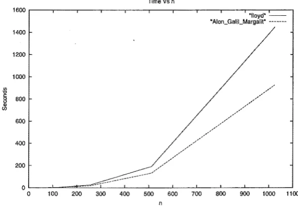
This Alon-Gali-Margalit algorithm was run against the Floyd's algorithm pre-sented above, see Figure 2.5. Strassen's distance matrix multiplication algorithm of time complexity O(n°·83 ) was used to perform the matrix multiplication. The graph clearly shows the AGM algorithm is better than Floyd.

1600

1400

1200

1000

"' "

~

800

(j)

600

400

200

0

Time Vs n

'floyd'--"Aion_Gaiii_Margalll'

---100 200 300 400 500 600 700 800 900 1000 1100

[image:10.595.131.433.325.534.2]

n

Figure 3.2: Results from comparing the two algorithms

3.2 Non-negative Real Numbers

(11)

Takaoka and Cook

3.3 Algorithm for Graphs with Small Edge Costs

The third algorithm uses the same cruising phase as the previous algorithm, but uses a different accelerating phase. The accelerating phase for this algorithm only works if the edge cost is small with this algorithm the edge cost must be

n°·

624 _{where n}_is_{the number of nodes in the graph. The largest edge cost} must be kept at this value in order to keep the overall algorithm at sub-cubic time complexity. The number of nodes in the graph is dependent on the size of the edge costs. As the edge costs increase the algorithm becomes slower. This dependency is due to the fact that Schonhage and Strassen's FFT algorithm is used[10]. This algorithm is able to solve the problem of multiplication on a k bit number in O(k log k log log k) time. This is quite an improvement over standard multiplication which has a time complexity of O(k2

). However this

improvement in time complexity is only noticed when the number of bits to be multiplied is greater than 1000. Timing these programs against other all pairs shortest path algorithms will not show any decrease in time complexity until numbers consisting of 1000 bits or more are used. The time complexity of this algorithm is O(M!n~(log n)~(log log n)!). This algorithm is dependent on

M, the largest value in the distance matrix.

3.3.1 Decrease in Time Complexity

As discussed in the previous subsection any decrease in the size of the edge costs in the matrix will decrease the time complexity and hence the size of the maximum edge cost which at present is at

n°·

624_•_{A small increase in efficiency} for this algorithm has been discovered. If the edge costs fall between

n°·

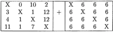
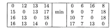
624 _and some other integer less than this but greater than zero, then by subtracting off this smaller value you are left with a smaller number, which as discussed earlier provides for some increase in efficiency, due to the fact you may now need less bits to store that number.

An example of this in effect is as follows. If you look at the matrix in Figure 3.3, the minimum value in this matrix is 6, as the zeros in the matrix represent an edge from the node back to the same node they are not taken into consideration. The solution to the all pairs shortest path problem for the matrix is given in Figure 3.4.

The maximum value in the matrix is 18. 18 requires 5 bits to be represented as the binary number 10110. After subtracting off 6 from all the values in the matrix you are left with a new matrix shown in Figure 3.5. The largest value in this new matrix is now 12 which requires only 4 bits to be represented as the binary number 1100.

The calculation of the algorithm can be performed on the reduced matrix in Figure 3.5. This reduced matrix consists of the matrix and the offset matrix. The offset matrix contains the number subtracted off of the original matrix. The matrix after completing one matrix multiplication is shown in Figure 3.6. After further repeated squaring the same matrix as Figure 3.6 is found.

(12)

It is trivial to show that the extra three steps of performing the subtracting, the addition and the min operator all take O(n2₎_{time, so they can be absorbed} into the dominant part of the algorithm which is the matrix multiplication.

Very little increase in efficiency is obtained from this algorithm because in many cases there may be a large gap between the smallest and largest numbers in the graph. This algorithm is dependent on the length of the number range, if the range is small, some decrease in time complexity could be observed and if the range is large, then little decrease in time complexity would be observed. However this did lead us to discover Spectral graph theory which is presented in the next chapter.

[image:12.595.243.329.255.308.2]

0 6 16 8 9 0 7 18 10 7 0 18 17 7 13 0

Figure 3.3: The initial matrix

0 '6 13 8

9 0 7 17

[image:12.595.194.378.460.512.2]

10 7 0 18 16 7 13 0

Figure 3.4: Solution using 3rd algorithm

X 0 10 2 X 6 6 6 3 X 1 12

₊

6 X 6 6

4 1 X 12 6 6 X 6

11 1 7 X 6 6 6 X

(13)

Takaoka and Cook

X 0 1 2 X 12 12 12

3 X 1 5

₊

12 X 12 12

4 1 X 6 12 12 X 12

[image:13.595.190.379.183.233.2]

4 1 2 X 12 12 12 X

Figure 3.6: The matrix after the first multiplication

0 12 13 14 0 6 16 8

15 0 13 17 min 9 0 7 18

16 13 0 18 10 7 0 18

[image:13.595.170.387.379.435.2]

16 13 14 0 17 7 13 0

Figure 3.7: The matrix after performing addition

0 6 13 8

9 0 7 17

10 7 0 18 16 7 13 0

[image:13.595.241.326.582.637.2]

(14)

Chapter

4 Spectral Graph Theory

4.1 What Is Spectral Theory

Spectral graph theory essential is an expansion of the idea presented in section 3.3.1. The difference between the first idea is that under the idea of subtracting off the smallest number in the graph this graph has one range. Under spectral theory further investigation of the graph is required. So as to find more ranges rather than just the one which is used in the first.

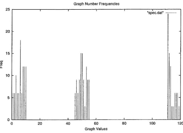
Then the matrix is split into these sub-ranges and the smallest value in each range is subtracted off. This means that for the purposes of algorithm 3 from section 3.3 the largest number in the graph is the largest range length. These ideas can be displayed in the graph in Figure 4.1. This graph displays the frequencies of the edge costs contained in a graph. This sort of graph displays the ideal properties that a graph would want in order to take advantage of this new algorithm presented in this chapter.

4.2 New Algorithm - Spectral Analysis of

Ma-trices

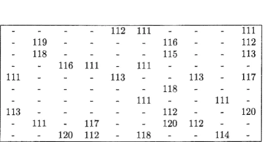
The outline for this new algorithm is as follows. The distance matrix is split into various sub matrices depending on which range the value falls into. Each value will fall into just one specific range as the example in Figure 4.2 shows, there are three ranges; range one is from 1 to 10; range two is from 45 to 55; range three is from 110 to 120. Figure 4.3 shows the distance matrix produced by retaining all the values for the first range and replacing all the values that fall into the other two ranges with infinity. The same thing has been done for the other two ranges and is shown in Figures 4.4 and 4.5.

(15)

Takaoka and Cook

Graph Number Frequencies

25,---,---~---.---~---r---. 'spec.dat' 20 15 10 5 o~~~~---~ o 1 46 54 4 111 50 51 113 9 6

20 40 60

Graph Values

[image:15.595.139.438.129.346.2]

80 100

Figure 4:1: An example of a Good Spectral graph

47 4 6 112 111 46 49 51

119 54 10 8 6 116 3 52

118 50 45 46 9 115 8 46

5 116 111 49 111 1 48 49

48 8 3 113 55 10 113 50

53 9 49 50 53 118 5 54

7 51 53 49 111 3 10 111

2 3 6 8 2 112 55 46

111 45 117 48 47 120 112 53

10 120 112 6 118 7 3 114

Figure 4.2: An example of a distance matrix

120 111 112 113 6 117 8 9 120 50 55

the maximum edge cost for the algorithm from section 3.3 was O(n°·624 ), this bound is now no longer the size of the graph but now is the maximum range length.

The repeated squaring of the matrix, which has 2 ranges, looks like this

(A

+

Dt min B

+

D2)(A

+

min B

+

D2). This is expanded to (A2

₊

2D1)min(AB

+

D1

+

D2)rnin(BA

+

D1

+

D2)min(B2

+

2D2).

4.3 A Problem With This New Algorithm

(16)

1 4 6

10 8 6 3

9 8

4 5 1

-

6

8 3 10

9 5

-

8

7 3 10

-

9

2 3 6 8 2

9

[image:16.595.138.404.126.692.2]

6 10

-

6 7 3

Figure 4.3: Sub-Range one

47 46 49 51

46 54 52

54 50 45 46 46

49 48 49

48 55 50

50 53 49 50 53 54

51 51 53 49

55 46

45 48 47 53 50

[image:16.595.189.378.147.272.2]

55

Figure 4.4: Sub-Range two

112 111 111

119 116 112

118 115 113

116 111 111

111 113 113 117

118

111 111

113 112 120

111 117 120 112

120 112 118 114

[image:16.595.146.417.525.671.2]

(17)

Takaoka and Cook

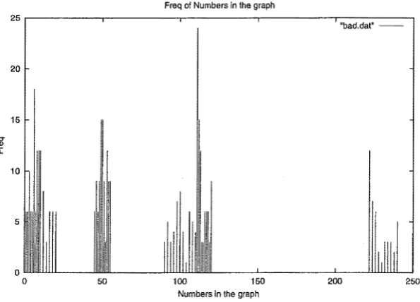
have doubled. So the bands could very quickly merge together as one and then you would no longer be able to use this algorithm. This can be visualised by firstly looking at the graph in Figure 4.1 which shows 3 ranges of numbers, the next graph, see Figure 4.6, shows what could have happened to that same graph after one matrix multiplication. Each of the ranges has spread out and with further multiplications the ranges would become more and more bunched together.

Freq of Numbers In the graph

25,---.---~.---~.---,---.

"bad.dat'

20

15

150 200 250

[image:17.595.135.433.227.441.2]

Numbers In the graph

(18)

Chapter 5 Two-band Algorithm

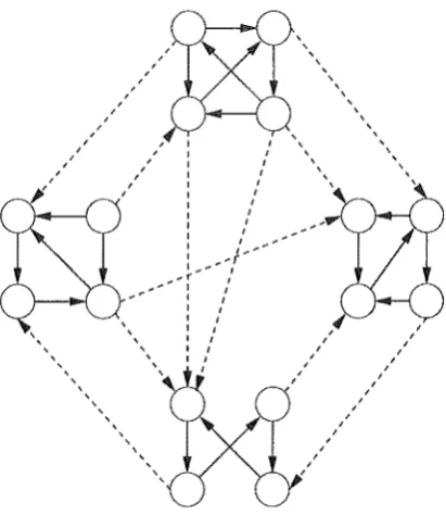
Expanding on these graph concepts presented in the previous chapters is the 2-band modified Floyd algorithm. This algorithm takes a two band approach, where as the algorithm from the previous chapter took a n band approach. Under this approach the graph consists of small sub-graphs that are then con-nected to each other to make up the entire graph. This can be demonstrated in Figure 5.2. If the reader looks at this figure they would be able to see that the graph consists of four sub-graphs, that are interconnected with each other. A requirement for each sub-graph is discussed in section 5.1.

Each of these individual subgraphs can then be calculated using Floyd's algorithm. then the overall graph can be calculated using a modified Floyd's algorithm. This algorithm is presented in the next section. Floyd's algorithm was presented in the second chapter of this report.

5.1 Requirement For the Sub-graph

Each node must have a path which has a specific length between each other node. This means that after each single node has been calculated the solution matrix for this sub-graph must have all values falling within a specific range.

5.2 The Two-band Algorithm

For a graph that consists of k sub-graphs each of the k sub-graphs is calculated using Floyd's algorithm presented in the first chapter. This is displayed below in the next piece of code. The algorithm is just Floyd's algorithm except for the first line which represents the algorithm being run over the k sub-graphs. This part of the algorithm has a time complexity of 0(

fk

3_),_{this is reduced to} O(nk2

).

1 for p

=

1 to n/k 2 for i

₌

1 to k 3 for j

=

1 to k

4 for 1 = 1 to k

5 M[i] [j]

=

M [j] min

(19)

Takaoka and Cook

This next piece of code shows the modified Floyd algorithm. This algorithm is basically the same as the original Floyd's algorithm, but in line 4 a matrix multiplication is ~erformed instead of an addition. The time complexity of this algorithm is 0( ~) for the first 3 lines and line 4 requires time complexity of O(k3

) for the matrix multiplication. When these two are combined and reduced an overall time complexity of O(n3

) is found. This second part of the algorithm is more dominant than the first part of the algorithm and so the first part of the algorithm can be absorbed into the second.

1 for i

=

1 to n/k do 2 for j

=

1 to n/k do 3 for 1

=

1 to n/k do

4 Matrix[i] [j]

=

Matrix[i] [j] min Matrix [i] [1]

*

Matrix [1] [j

J ;

This leaves the algorithm having the same time complexity as that of Floyd's algorithm. A way of decreasing the time complexity of this algorithm would be to subtract the minimum value off of the sub-graphs and use algorithm 3 from section 3.3. If this algorithm is used for the multiplication then a decrease in the time complexity could be achieved due to the fact that the numbers in the sub-graph would be using less bits.

Algorithm 3 had a relationship based on the size of the largest edge cost called m. line 4 can be performed in O(f(m, k). This would then lead to an overall time complexity of O(f(m,k)(ft)3

). As long as the function

f

is kept below

k+

then a decrease in time can be achieved by this algorithm.

-

~> ',V\ [6]

5.3 Deciding

How

To Split The Subgraphs

Splitting these bands into the various sub-graphs is not an easy task. Mathe-matically it must be such that each sub-graph must only go from one point in the sub-graph to every other point in the sub-graph without using an edge that exists outside of the sub-graph. If M is the length of the longest path in this sub-graph then all edges leaving or entering this sub-graph must have a value greater than M

+

2. There is no algorithm for finding these sub-graphs without using to much time up so the sub-graphs that the author was worldng with had sub-graph longest path of the

Vn·

The length of the shortest path leaving this sub-graph was n. These points raised in this section can be demonstrated in

figure 5.1.

5.4 Predictable Gain

Comparing this algorithm's time complexity with that of say Floyd's for graphs where the sub-graph has largest edge cost of

vn

has a time complexity the same as that of Floyd's, Floyd's has time complexity of O(n3

) and this algorithm has time complexity of O(n3

) as discussed in section 5.2.

(20)

I

/,,."'"'"'

I

Subgraph

• Edge leaving the subgraph.

I I I I I I I r-,

I ',,

'

...,._--

-~- '

' _' ' _'_I

I I I I I I I I I ' _' _-~---'

' I

\ \ " 1/F

~,

I "',

,..I-,...-11 ... _-'"' ... I

I I

I I I

[image:20.595.173.378.140.374.2]

Edge entering the subgraph.

Figure 5.1: Demonstrating how the subgraphs are split

~~\,

I \

I '

I \

I \ \

I 1 I I \ '

I 1 1 I \ \

11 I 1 I \ '..,

.,~'"' ,''

:

,' ',, ',

p I : i

', ' ' ' _' ', ' _' \ \

--', ' \ ' \ \ '

I I

I I .,..,.""

I I .,..,.. I I ~"' I _.f ... ""

1.., ... ,

' r I

I I

l I

I I

I 1

I I

I I I I

I I I I I I I I I I I I I I I I I I I I

[image:20.595.175.381.441.679.2]

(21)

Chapter 6 Maximum Sub-Array

problem- An application of

The All Pairs Shortest Path

As an aside to the work from the previous chapters. The maximum sub array problem, which involves maximising the negative and positive numbers in a matrix, so as to choose that part of the matrix which has the largest sum in it. This is trivial in a matrix that contains only positive numbers as naturally it will be the sum of the whole matrix. But when that matrix contains negative and positive numbers then another kind of algorithm will have to be used. The brute force algorithm for solving this has a time complexity of O(n4_)._Recently this problem was shown to be equivalent to the all pairs shortest path problem. This algorithm is therefore a perfect example of another good use for the all pairs shortest path algorithms. The maximum sub-anay problem can be used as an efficient algorithm for data mining of information and for identifying the brightest portion of an image.

6.1 Maximum Sub Array Algorithm

This algorithm is a divide and conquer type algorithm and only the outer frame is presented, for an in depth look at the algorithm see the paper by T. Takaoka [11] or the paper by H. Tamaki and T. Tokuyama[12].

The Algorithm selects the overall solution from the maximum of the six solu-tions given below. The solusolu-tions for the NW,SW,NE,SE parts of the matrix are given by recursively calling the algorithm on these parts. The row centred prob-lem and the column centred probprob-lem is when the maximum sub-array crosses either the vertical or horizontal dividing lines. The algorithms for solving both these problems is given in the paper by T. Takaoka[ll].

• Anw Solution for the NW part of the matrix.

• Asw Solution for the SW part of the matrix.

(22)

• Ase Solution for the SE part of the matrix.

• Arow Solution for the row-centred problem.

e Acolumn Solution for the column-centred problem.

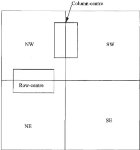
This is illustrated in the diagram that shows the matrix split into its various parts. This diagram is found in figure 6.1.

The relationship between this problem and the all pairs shortest path prob-lem is in the solution to the column centre and row centre. Both these can be reduced to the all pairs shortest path problem.

Column-centre

I

v

NW

sw

Row-centre

SE NE

Figure 6.1: Diagram illustrating the splitting of the matrix

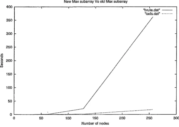
6.2 Results

[image:22.598.143.419.258.553.2]

(23)

Takaoka and Cook

Their is further work required in this field to try different All pairs shortest path algorithms for this maximum sub array problem and test to see which are more effective.

400

350

300

250

"'

"tJ

§ 200

.,

(f)

150

100

50

0

0 50

New Max subarray Vs old Max subarray

'brute.dat' -'tads.dat' ---·

_____ ,.. ~ .. ---~ ..

---~---..--100 150

Number of nodes

[image:23.595.133.433.178.391.2]

200 250

Figure 6.2: Results for the maximum sub array problem

(24)

Chapter 7 A Graphical Front End For

Displaying Graph

Algorithms

A Graphical user interface for displaying these graph algorithms at work is under development. This would allow the user the ability to display a graph algorithm running and to show the path calculated by the all pairs shortest path algorithm that user has selected to display. Currently this is written in the TCL /TK language with an adaption to the TCL interpretor so as to allow it to handle matrices. The Figure 7.1 displays a screen-shot of the graphical front end. In this you can see a graph entered into the canvas widget. There are large buttons to select either nodes or lines, which the user could then draw onto the canvas widget. A user can select a line and then type in the entry box a value for that edge. When the multiply button is hit the program goes off and calculates the all pairs shortest path problem. This program uses a different algorithm depending on what the user has selected from the Algorithm menu.

7.1 Future Development

(25)

Takaoka and Cook

[image:25.598.148.422.258.562.2]

(26)

Chapter 8 Conclusion

In this report the author has presented the user with a number of new approaches to deal with the all pairs shortest path algorithm. These new approaches are to do with looking at the structure of the graph and then using this information so as to gain further decreases in time complexity.

The approach taken in this project was to take the original algorithm, 3rd algorithm presented in Takaoka's paper (6]. The first approach found that you could subtract off the minimum value from the matrix and therefore benefit from a very small decrease in the time complexity.

Then we went on to look at spectral graph theory, which involves splitting the graph into various bands or ranges of numbers, separating the graph into many separate graphs consisting of these bands, using a modified algorithm of algorithm 3 and finally putting the whole thing back together as the solution matrix. In this approach you gain efficiency from the subtracting off of the lower bound for each range. This algorithm however had a draw back as discussed in section 4.3.

Finally the Algorithm from chapter 5 was discovered which is again further refinement of the work done in the previous chapter. This algorithm was able to take graphs with a specific structure and use this structure so as to gain a decrease in the time complexity of the algorithm by malting use of the algorithm 3 discussed in chapter 3.

So in concluding many authors looking into the problem of the all pairs shortest path have come up with a number of algoritluns that deal with the structure of the graph, these algorithms were however dealing with things such as sparse graphs and acyclic graphs. Not much work has been done actually looking at the overall edge costs and how these edge costs interact. There is certainly a lot more work in this field of spectral analysis of graphs for another researcher to look into.

8.1 Further Work

(27)

Takaoka and Cook

(28)

Appendix A

(29)

Takaoka and Cook

#include "strassen.h" #include "tad.h" #include <time.h> #define MAX 1000 int **A·**B; int **SOll,**SOl2;

int makematrix(int n,double p) { int i,j;

}

double temp; for(i=O;i < n;i++) {

}

for(j=O;j < n;H+) {

}

temp (double) ((rand() %MAX) + 1); temp

=

temp / (double) MAX;

if(temp >= p) { A[iJU]

=

2; } else {

A[iJUJ

=

INF; }

A[i][iJ = 1; if(i != (n-1)) {

A[i][i+1] = 2;

} else { A[ij[O] = 2;

}

return 0;

int printmatrix(int **A.int n) { int i,j;

}

printf("\n"); for(i=O;i<n;i++) {

}

for(j=O;j<n;H+) { printf("%4i" ,A[iJD]);

}

printf("\n"); printf("\n"); return 0;

int main(int argc,char Mrgv[J) { time_t t;

clock_t c; int n,i,j; double p; if(argc != 3) {

}

fprintf(stderr,"%s int double\n",argv[O]); exit(l);

if ((n = atoi(argv[lJ)) == 0) {

fprintf(stderr, "The first parame~ must be an integer\n"); exit(1);

}

if ((p atof(argv[2))) 0) {

(30)

#include "strassen.h"

int ** M_Matrix(int n.int one, int two) { int i,j;

}

int **temp;

temp malloc(sizeof(inh) * n); if( temp NULL) {

}

perror("Malloc Failed\n"); exit(1);

for(i=O;i<n;i++) {

}

temp[i] = calloc(n,sizeof(int)); if(temp[i] == NULL) {

perror("Malloc Failed\n"); exlt(1);

}

if(two != -1) { for(j=O;j<n;j++) {

temp[i]UJ = two; }

}

if(one != { temp[i] [i] one; }

return temp;

void free_m(int **t,int n) { int i;

}

for(i=O;i<n;i++) { free( t [i]);

}

free( t );

int strassen (int **solution,int **A, int **B, int n) { int halfn n/2;

int **M1,**M2,**M3,**M4,**M5;

int **M6,**M7,**Anew,**Bnew; int i,j;

M1 = M_Matrix(halfn,-1,-1); M2 M_Matrix(halfn,-1,-1); M3 M_Matrix(halfn,-1,-1); M4 M_Matrix(halfn,-1,-1); M5

=

M_Matrix(halfn,-1,-1); M6

=

M_Matrix(halfn,-1,-1); M7

=

M_Matrix(halfn,-1,-1); Anew = M_Matrix(halfn,-1,-1); Bnew M_Matrix(halfn,-1,-1); 29 if(n

==

2) {

M1[0J[O] (A[OJ[1] - A(1][1]) * (B[1)[0] + B[1)[1l); M2[0][0] (A[OJIO] + A[1][1l) * (B[OJ[O] + B[ll[1]); M3(0][0]

=

(A[O][O] A(1][0]) * (B[O][O] + B(0][1]);

(31)

Takaoka and Cook

#include "tad.h" #include "strassen.h" #include <stdlib.h> #include <stdio.h> #include <math.h> void test() {

return; }

double 1ogb( double x,double b) { return log(x) /log(b);

}

int pmatrix(int **A,int n) { int i,j;

}

for(j=O;j<n;j++) { printf("%4i 11 _,A[iJD]);

}

printf(11_\n11 );

printf("\n"); return 0;

int round(double x) { int i;

}

(int) x;

x x - (double) i; if(x >= 0.5) {

+

1;

} return i;

int A_G_M(int **D,int **A, int n,float r) { int l,i,j;

int **B·**C; int flag; flag= 0;

B M_Matrix(n,1,-1); C M_Matrix(n,-1,-1); for(l=2; 1 <= (int) r;l++) {

if(flag

==

0) { strassen(C,A,B,n); for(i=O; i < n; i++) {

for(j=O;j<n;j++) {

if(

C[iJUJ

>

1) {

CliJUJ

= 1;

} } } } else {

strassen(B,A,C,n); for(i=O; i < n; i++) {

for(j=O;j<n;j++) { if(B[iJUJ

>

1) {

(32)

#define MAX 512 #define INF 999 #include <stdlib.h> #include <stdio.h> #include <sysftypes.h> #include <time.h>

typedef int Matrix_t[MAXJ[MAX]; Matrbct a,b,u,v,w,s,t,sum,column,temp;

void subarray(int ml,int m2,int nl,int n2,int *value); void mult(int a,int b,int c,int d,int *Value);

int max(int xl,int x2,int x3,int x4,int x5,int x6);

void mult(int a,int b,int c,int d,int *Value) { int i,j,k,l,m,n;

Matrix_t suml; m

=

b-a+l; n = d-c+l;

for(i=1;i<=m;i++) { for(j=1;j<=n;j++) {

sum1[iJU] temp[a+i-l][c+j-1]; }

}

for(i=1;i<=n;i++) { for(j=l;.i<=n;j++) {

} }

s[i)[O] O;s[O]U] 0;

t[i](O] O;t[OJUJ 0; s[iJD) sum1[iJU); t[i]UJ = -sumlU][i];

for(i=1;i<=m;i++) { for(k=O;k<=m;k++) {

} }

w[i][kj INF;

for(l=O;l<=(n / 2 1 );1++) { if((s[i][l] + t[l][k]) < (w[i][k])) {

w[i][k] s[iWJ + W][k]; }

}

for(i=1;i<=m;i++) { for(j=l;j<=m;j++) {

if(i<=j) { w[iJU] = INF; }

} }

for(i=l;i<=m;i++) {

for(j=(n/2+1);j<=n;j++) {

v(iJU] = INF; 31

for(k=O;k<=m;k++) {

}

(33)

Takaoka and Cook

#!/users/ case/honours/ djc110/ Cosc460/tixScriptfmytcl -f

set menuframe .menufr set filebut $menuframe.file set algobut $menuframe.algo set fileMenu $filebut.f set algoMenu $algobut.f set mainframe .mainfr set iconframe .iconfr

set myc $mainframe.mycanvas set butCircle $iconframe.cir set butMul $iconfrarne.mul set butLine $iconframe.line set textbx $iconframe. txt set Matrix [NewMatrix] set node 0

set cir 1 set line 2

set currline(val) 0 set currline(xval) 0 set currline(yval) 0 set currline(xlast) 0 set currline(ylast) 0 set currnode 0 set OPT(width) 500 set OPT(height) 460 set OPT(mnhgt) 40

set OPT(cirfile) "Ndjc110/Cosc460/tixScript/cir .gif" set OPT(linefile) "-djc110/Cosc460/tixScript/line .gif" set OPT(SaveFile) 0

set OPT(LoadFile) 0 set number 0 set NODES 0 set Row 0 set Col 0

10

20

30

frame $mennframe -width $0PT(wldth) -height $0PT(mnhgt) -relief raised -bd 3 frame $mainframe -width $0PT(width) -height $0PT(height)

frame $iconframe -width $0PT(width) -height $0PT(mnhgt) -relief raised -bd 3 menubutton $filebut -text "File" -menu $fileMenu

menubutton Salgobut -text "Algorithm" -menu $algoMenu 40 menu $fileMenu

menu $algoMenu

image create photo $cir -file $0PT(cirfile) image create photo $line -file $0PT(linefile)

button $butCircle -image $cir -command "Nodes $myc" -bd 1 -relief flat button $butLine -image $line -command "Lines $myc" -bd 1 -relief flat button $butMul -command "runMul" -text "Multiply"

canvas $myc -relief groove -bd 3 -width $0PT(width) -height $0PT(height) entry $textbx -textvariable number -state disabled

bind $textbx <KeyPress-Return> "TextEnter"

$fileMenu add command -label "New" -command {New}

$fileMenu add command -label "Save Fila . . . " -command {Save} $fileMenu add command -label "Load File . . . " -command {Load} $fileMenu add command -label "Quit" -command {exit}

32

proc New{} {

global Matrix node set i 1

50

(34)

#include <tk.h> #ifndef MATRIX_H #define MATRIX_H

void init_Matrix(int n);

int NewMatrix(ClientData clientData, TcLinterp *interp, int argc, char *argv[]);

int delMatrix( ClientData clientData, TcLinterp *interp, int argc, char *argv[]);

int set Matrix( ClientData clientData, TcLinterp *interp, int argc, char *argv[]); int get Matrix( ClientData clientData,

TcLinterp *interp, int argc, char *argv[]);

int SizeMatrix( ClientData clientData; TcLinterp *interp, int argc,char *argv[]);

int setNodePos(ClientData clientData, TcLinterp *interp, int argc,char *argv[]);

int getNodePos(ClientData clientData, TcLinterp *interp, int argc,char *argv[]);

int getNodeVal(ClientData clientData, TcLinterp *interp, int argc,char *argv[]);

int setNodeVal(ClientData clientData, TcLinterp *interp, int argc,char *argv[]);

int getLines( ClientData clientData, TcLinterp *interp, int argc, char *argv[]);

int getNode(ClientData clientData, TcLinterp *interp, int argc,char *argv[]);

int getLine( ClientData clientData, TcLinterp *interp, int argc, char *argv[]);

int setLine( ClientData clientData, TcLinterp *interp, int argc, char *argv[]);

int MatrixMul(ClientData clientData,TcLinterp *interp, int argc, char *argv[]); 33

#endif

10

20

30

40

(35)

Takaoka and Cook

int writeout(int n,int r,int *a,int **m,char *f); int inrange(int n);

int center(int c,int n);

int ** makematrix(int n,int r,int *ranges,ftoat *Weights); int printmatrlx(int **matrix,int n);

(36)

#include <stdlib.h> #include <stdio.h> #include <string.h> #include <sysltypes.h> #include <time.h> #include "matrix .h" #include "create.h"

int writeout(int n,int r,int *a,int **m,char *f) { FILE *ptr;

} inti;

if(strcmp(f,"stdout")

==

0) { ptr = stdout;

} else {

ptr = fopen(f,"w"); if(ptr ==NULL) {

return -1; }

}

fwrite( &n,sizeof(int ), 1 ,ptr); fwrite(&r,sizeof(int),1,ptr); fwrite( a,sizeof( int ),r ,ptr ); for(i=O;i < n;i++) {

fwrite(m[i],sizeof(int ),n,ptr ); }

return 0;

int inrange( int n) { float c,r;

}

c = 1

I

(float) n;

r = (float) (random() % 100000)

I

100000.0; return (int) (r

I

c);

int center(int c,int n) { int number;

}

number = inrange(n); if(inrange(2)) {

number

=

0 - number; }

return c + number;

int ** makematrix(int n,int r,int *ranges,float *Weights) { int **matrix;

} int i,j;

matrix newMatrix(n); for(i=O;i<n;i++) {

for(j=O;j<n;j++) { 35

} }

matrix[iJU] center(ranges[inrange( r) ],10 );

return matrix;

10

20

30

50

(37)

Talcaoka and Cook

#ifndef CREATE_H #define CREATE-H int ** newMatrix(int n); #endif

Figure A.9: Source Code for create.h

#ifndef SPEC_H #define SPEC_H

int setup(int n,int r,int **M);

int ** spectral(int n,int r,int *rang,int **M); int ** normal(int n,int **M);

int isrange(int n,int a,int l);

int divide(int n,int r,int *rang,int **M);

int multiplySpec(int n,int i,int j,int r,int Hang,int **M,int 1); int check(int n,int **spec,int **nor);

#end if

Figure A.lO: Source Code for spec.h

(38)

#include <stdlib.h> #include <stdio.h>

int main(int argc,char *argv[]) { FILE *Ptr;

}

int n,r,*range; int **M,i,j;

ptr = fopen(argv[l],"r"); fread( &n,sizeof(int ).l.ptr ); fread( &r,sizeof(int ),l,ptr);

range (int *) malloc(sizeof(int) '* r); fread( range,sizeof(int ),r,ptr );

M

=

(int **) malloc(sizeof(int*) * n); for(i=O;i <n;i++) {

}

M[i] = (inh) calloc(n,sizeof(int));

fread(M[i],sizeof( int) ,n, ptr);

printf("\nNodes: %i ",n); printf("Ranges %i \n",r); for(i=O;i<r;i++) {

printf("%4i ",range[i]); }

}

for(j:=O;j<n;H+) { printf("%4i ".M[i)[i]);

}

printf("\n"); return 0;

Figure A.ll: Source Code for testm.c

10

20

(39)

Bibliography

[1] F. Romani. Shortest-path problem is not harder that matrix multiplica-tions. Inform. Process. Lett., 11:134-136, 1980.

[2]

Tadao Takaoka. A new upper bound on the complexity of the all pairs short-est path problem. Information Processing letters, 43(6):195-199, September 1992.

[3]

T. Takaoka. Shortest path algorithms for nearly acyclic directed graphs.

Theoretical Computer Science, 203:143-150, 1998.

[4] A. Moffat and T.' Takaoka. An all pairs shortest path algorithm with expected time o(n2_log_n)._SIAM_J._Comput.,_{16:1023-1031, 1987.}

[5] R.W. Floyd. Algorithm 97: Shortest path. Comm. ACM, 5:345, 1962.

[6]

Tadao Takaoka. Subcubic cost algorithms for the all pairs shortest path problem. Algorithmica, 20:309-318, 1998.

[7]

N. Alon,

Z.

Galil, and

0.

Margalit. On the exponent of the all pairs shortest path problem. Proc. 32nd lEE FOGS, pages 569-575, 1991.

[8] D.

Coppersmith and S. Winograd. Matrix multiplication via arithmetic progressions. J. Symbolic Gomput., 9:251-280, 1990.

[9] V.

Strassen. Gaussian elimination is not optimal. Numerische Mathematik, 13:334-6, 1969.

[10} A. Schonhage and V. Strassen. Schnelle multiplikation grosser zahlen.

Com-puting., 7:281-292, 1971.

[11] T. Takaoka. An efficient algorithm for data mining based on the maximum subarray problem. 1999.

[12] H. Tamaki and T. Tokuyama. Algorithms for the maximum subar-ray problem based on matrix multiplication. Proceedings of the 9th SODA(Symposium on Discrete Algorithms)., pages 446-452, 1998.

All Pairs Shortest Path Algorithms