doi:10.1093/imamat/xxx000
On the inverse problem for Channell collisionless plasma equilibria
OLIVERALLANSON∗
Space and Atmospheric Electricity Group, Department of Meteorology, University of Reading, Reading, RG6 6BB, UK.
Solar & Magnetospheric Theory Group, School of Mathematics & Statistics, University of St Andrews, St Andrews, KY16 9SS, UK.
∗Corresponding author: [email protected]
SASCHATROSCHEIT
Department of Pure Mathematics, Faculty of Mathematics, University of Waterloo, Waterloo, N2L 3G1, Canada.
Analysis Group, School of Mathematics & Statistics, University of St Andrews, St Andrews, KY16 9SS, UK.
AND
THOMASNEUKIRCH
Solar & Magnetospheric Theory Group, School of Mathematics & Statistics, University of St Andrews,
St Andrews, KY16 9SS, UK. [email protected]
[Received on 14 April 2018]
c
Vlasov-Maxwell equilibria are described by the self-consistent solutions of the time-independent Maxwell equations for the real-space dynamics of electromagnetic fields, and the Vlasov equation for the phase-space dynamics of particle distribution functions (DFs) in a collisionless plasma. These two systems (macroscopic and microscopic) are coupled via the source terms in Maxwell’s equations, which are sums of velocity-space ‘moment’ integrals of the particle DF. This paper considers a particular subset of solutions of the broad plasma physics problem: ‘the inverse problem for collisionless equilibria’ (IPCE), viz. “given information regarding the macroscopic configuration of a collisionless plasma equilibrium, what self-consistent equilibrium DFs exist?” We introduce the constants of motion approach to IPCE using the assumptions of a ‘modified Maxwellian’ DF, and a strictly neutral and spatially one-dimensional plasma, and this is consistent with ‘Channell’s method’ (Channell, 1976). In such circumstances, IPCE formally reduces to the inversion of Weierstrass transformations (Bilodeau, 1962), such as those transformations that feature in the initial value problem for the heat/diffusion equation. We discuss the various mathematical conditions that a candidate solution of IPCE must satisfy. One method that can be used to invert the Weierstrass transform is expansions in Hermite polynomials. Building on the results of Allanson et al. (2016), we establish under what circumstances a solution obtained by these means converges, and allows velocity moments of all orders. Ever since the seminal work by Bernstein et al. (1957), on ‘stationary’ electrostatic plasma waves, the necessary quality of non-negativity has been noted as a feature that any candidate solution of IPCE will nota priorisatisfy. We discuss this problem in the context of Channell equilibria, for magnetised plasmas.
Keywords: Insert keyword text here.
1. Introduction
It is estimated that more than 99% of the observable matter in the universe is in the plasma state. These plasmas are frequently sufficiently hot and/or diffuse that the particles rarely collide, for example the collisionalmean free pathin the solar wind is approximately equal to the distance from the Sun to the Earth (e.g. see Marsch & Goldstein (1983); Marsch (2006)). In such circumstances, the plasma dynam-ics can be accurately modelled without including collisions (e.g. see Schindler (2007); Belmont et al. (2013)). Collisionless plasmas behave quite differently to collisional plasmas, and are best modelled using the Vlasov kinetic theory of particle distribution functions (DFs) in position-velocity phase space (e.g. see Krall & Trivelpiece (1973); Chen (2015)), rather than collisional fluid models that operate in position space only (e.g. see Kulsrud (1983); Freidberg (1987) for discussions of the Magnetohydrody-namic theory).
In nature, this difference is made manifest by the critical dependence of the macroscopic dynamics of collisionless plasmas on the velocity space structure of particle distributions (Gary, 2005), and on the short length and time scale physics of collisionless processes (e.g. see Lifshitz & Pitaevski˘ı (1981); Kulsrud (2005); Schindler (2007)). Modern instrumentation is now able to make observations of par-ticle distributions with spatio-temporal resolution on kinetic scales, for example the NASA Multiscale Magnetospheric (MMS) mission (Hesse et al., 2016). As such, it is of interest and importance to plasma observers, modellers and theorists to better understand the micro-scale kinetic physics of collisionless plasmas, and in particular how this relates to the macroscopic dynamics, which are typically better understood.
macroscopic physics (e.g. see Drake & Lee (1977); Daughton (1999)). Due to the technical difficulty in calculating exact Vlasov equilibria, approximate solutions are often used as initial conditions instead of exact solutions (e.g. see Swisdak et al. (2003); Hesse et al. (2005); Pritchett (2008); Malakit et al. (2010); Aunai et al. (2013); Hesse et al. (2013); Guo et al. (2014); Hesse et al. (2014); Liu & Hesse (2016)), and it is not always known how far the approximate solution is from a true equilibrium. As such, it is of interest to modellers and theorists to better understand the equilibrium states of Vlasov plasmas. However, there is not a well-established ‘user-friendly’ theory that relates the equilibrium and stability properties of the macroscopic real-space description of the plasma to those of the microscopic phase-space description, in the sense of a ‘one-to-one’ correspondence, i.e. ‘micro↔macro’. Calcu-lating a kinetic equilibrium given some macroscopic conditions is an example of a non-unique inverse problem: ‘the inverse problem in collisionless equilibria’ (IPCE), viz. “given information regarding the macroscopic configuration of a specific collisionless plasma equilibrium, what self-consistent equi-librium distributions exist?” (e.g. see Channell (1976); Mynick et al. (1979); Harrison & Neukirch (2009b) for examples of IPCE solutions, and Allanson et al. (2016) for examples and discussion). This paper considers IPCE applied to spatially one-dimensional (1D) plasmas, and focuses in particular on the mathematical validity of 1D IPCE solutions.
This paper is structured as follows. In Section 2. we introduce the basic theory of the Vlasov equa-tion and the equaequa-tions of Vlasov-Maxwell equilibria. We discuss the two distinct approaches to calculat-ing self-consistent collisionless plasma equilibria (‘forward’ and ‘inverse’), and previous works on the non-negativity of DFs obtained in IPCE. Section 3. focusses on IPCE in spatially 1D plasmas; outlines parallels between the mathematical formalism of IPCE as presented, and the initial value problem for the heat equation; and introduces the Fourier transform method of formally inverting the equations in this formalism to obtain IPCE solutions. An alternative method to solve IPCE is to use expansions in Hermite polynomials, and this method is outlined in Section 4. One downfall of this method is that the non-negativity of expansions in Hermite polynomials is nota prioriknown. We present general results on the convergence of the Hermite polynomial expansions, and the existence of velocity moments of all orders, and we discuss the problem of non-negativity. In Section 5. we summarise the theory and results presented in this paper.
2. Basic Theory
2.1 The Vlasov Equation
The Vlasov equation (Vlasov, 1968) - also known as the collisionless Boltzmann equation - governs the evolution of the plasma DF for ‘particle’ speciess, fs, in six-dimensional phase-space,(xxx(t),vvv(t)). Here,xxxandvvv=dtxxx denote the particle position and velocity, respectively. The Vlasov equation can be used to model the statistical behaviour of collisionless particle distributions for rarefied gases and plasmas, or even to describe the distribution of stars (e.g. see Henon (1982); Pegoraro et al. (2015) for short introductions to some relevant literature and applications). The Vlasov equation is given in Cartesian geometry by
d
dtfs(xxx(t),vvv(t);t) =
∂fs
∂t + dxxx dt ·
∂fs
∂xxx + dvvv dt ·
∂fs
∂vvv =0. (2.1)
One can construct ‘macroscopic’ quantities in real-space by taking velocity-space moments of the DF. For example, the number density (a scalar), bulk flow (a vector), and pressure tensor (of rank-2) for speciessare given by
ns(xxx;t) =
Z
fsd3v, V
VVs(xxx;t) = n−s1
Z
vvv fsd3v, Pi j(xxx;t) =
∑
s ms
Z
(vi−Vi,s)(vj−Vj,s)fsd3v, (2.2)
formsthe mass of particle speciess, and
R
d3vthe integral over all velocity space, i.e.R3. In order for
the DF to be have physical meaning, one must be able to take at least as many velocity moments as a corresponding fluid theory requires, and the DF must be non-negative over all phase space. In this paper we define a physical DF as one which allows velocity-space moments of all orders, and so satisfies
Z
vixvyjvkz fsd3v
< ∞∀i,j,k∈0,1,2, ... (2.3)
fs(xxx,vvv,t) > 0∀(xxx,vvv,t). (2.4)
2.2 Vlasov-Maxwell equilibria
This paper will focus on the application to a fully ionised and non-relativistic ion-electron plasma, for which the electromagnetic forces dominate the collective behaviour of the plasma. We shall also ignore gravitational effects. In such circumstances, an individual particle of chargeqsand massmsis subject to the Lorentz force,
ms dvvv
dt =qs(EEE+vvv×BBB), (2.5)
for EEE andBBBthe self-consistent electric and magnetic fields respectively. A Vlasov equilibrium cor-responds to a statistically steady-state of the particle distribution, and is mathematically described by ∂tfs=0. Therefore, we see from equations (2.1) and (2.5) that a collisionless plasma equilibrium DFs obeys by the steady-stateVlasov-Maxwellequation,
vvv·∂fs
∂xxx
+qs
ms
(EEE+vvv×BBB)·∂fs
∂vvv
=0. (2.6)
Most typically (e.g. see Schindler (2007)), analytical equilibrium solutions of the Vlasov equation are constructed using a theorem attributed to Jeans (Jeans, 1915; Lynden-Bell, 1962). ‘Jeans’ theorem’ states that fsis a solution of the Vlasov equation if it is a function of a subset of thekknown constants of motion for particle speciess,
{Cn,s(xxx(t),vvv(t)):dtCn,s=0,n=1, ...,k}.
constants of motion,Cn,s(xxx,vvv), sinceCn,s may not be monotonic functions of(xxx,vvv)(e.g. see Belmont et al. (2012); Dorville et al. (2015) and references therein).
Whilst the steady-state Vlasov-Maxwell equation (equation 2.6) can trivially be solved by any func-tion of the constants of mofunc-tion (that also obeys equafunc-tions (2.3) and (2.4)), the challenge lies in the fact that the DF must also be self-consistent with the time-independent Maxwell equations,
∇·EEE = σ ε0
, (2.7)
∇×EEE = 000, (2.8)
∇·BBB = 0, (2.9)
∇×BBB = µ0jjj, (2.10)
for the speed of lightc= (µ0ε0)−1/2,ε0 the vacuum permittivity,µ0the vacuum permeability, σ the charge density, and jjjthe current density. Maxwell’s equations couple to the Vlasov-Maxwell equation through the source terms on the right-hand side (RHS) of Gauss’ law, and Amp`ere’s Law (equations (2.7) and (2.10) respectively):
σ(xxx) =
∑
s
qsns=
∑
sqs
Z
fsd3v, (2.11)
jjj(xxx) =
∑
qsnsVVVs=∑
sqs
Z
vvv fsd3v. (2.12)
Note that equations (2.8) and (2.9) are automatically satisfied for the electric fieldEEE=−∇φdefined as the (negative) gradient of the scalar potentialφ(xxx), andBBB=∇×AAAthe curl of the vector potentialAAA(xxx). An equilibrium solution of theVlasov-Maxwell systemis therefore characterised by a self-consistent set of DFs and potential functions,
{fs:s=i,e},φφφ(xxx),AAA(xxx),
such that equations (2.6), (2.7) and (2.10) are satisfied, with the subscriptsiandecorresponding to ions and electrons respectively (e.g. see Mynick et al. (1979); Greene (1993); Schindler (2007)).
2.3 The forward and inverse approaches
The Vlasov-Maxwell system is an integro-differential set of equations, and there are two different approaches that could be made to solve it. The one most typically seen is the ‘forward’ approach, in which one specifies the DFs, proceeds to calculate the source terms via the integrals in equations (2.11) and (2.12), and then attempts to solve the differential equations (2.7) and (2.10) forφandAAA(e.g. see discussions in Bennett (1934); Grad (1961); Harris (1962); Sestero (1964, 1965); Lee & Kan (1979); Schindler (2007); Kocharovsky et al. (2010); Vasko et al. (2013)). In this approach (‘micro’→‘macro’), one typically assumes a form of the equilibrium DF that is thought to be mathematically/physically reasonable, and frequently one of Maxwellian form,
fMaxw,s=
ns(xxx) (√2πvth,s)3
e−(vvv−VVVs(xxx))2/(2v2th,s),
ns,VVVs,jjj,Pi jetc (e.g. see Harris (1962); Schindler (2007); Vasko et al. (2013)). Whilst this approach is typically easier than the one that we are about to introduce, it has one significant drawback. In contrast to collisional plasmas for which there is in principle a unique equilibrium solution of the corresponding kinetic equation: the Maxwellian DF (Grad, 1949b), collisionless plasmas admit an infinity of possible equilibrium DFs (i.e. any function of the constants of motion). Hence, for the many man-made, terres-trial, space, solar and astrophysical plasmas in which the collisionality is insufficient to drive the DF to a thermal equilibrium Maxwellian DF, one does nota prioriknow what form of the DF on which to base their calculation.
The ‘inverse’ approach is the method that we shall focus on in this paper (‘macro’→‘micro’). In the ‘inverse problem for collisionless equilibria’ (IPCE), one specifies certain features of the macroscopic equilibrium configuration, e.g.BBBandEEE, and attempts to find a self-consistent DF (e.g. see discussions in Alpers (1969); Channell (1976); Mynick et al. (1979); Greene (1993); Harrison & Neukirch (2009b); Belmont et al. (2012); Allanson et al. (2016)). This approach involves the inversion of integral equations, and has two potential drawbacks. The first is that there are in principle infinitely many solutions to IPCE, and so one has to question whether the DF obtained by the chosen method is physically realistic, or just a mathematical curiosity. The second is that the equilibrium DF may not be able to be expressed in closed form, and the necessary conditions of equations (2.3) and (2.4) may be in question.
2.4 Previous work on non-negativity
The first body of works on IPCE (Bernstein et al., 1957; Montgomery & Joyce, 1969; Tasso, 1969; Schamel, 1971) mainly focussed on electrostatic configurations, i.e. EEE6=00 and0 BBB=000 (the Vlasov-Poisson system). In Bernstein et al. (1957), an inductive integral equation method is developed that calculates the DF of trapped electrons in a nonlinear travelling electrostatic wave ( Bernstein-Greene-Kruskal (BGK) waves), for a given 1D scalar potential,φ, in the wave frame. Whilst Bernstein et al. (1957) recognised that equation (2.4) must be satisfied for the DF to be physically meaningful, they did not formally explore this feature. Montgomery & Joyce (1969), Tasso (1969) and Schamel (1971) demonstrated that it is indeed possible to obtain non-negative trapped DFs for the trapped electron population, and this is relevant to the physics of nonlinear plasma waves (e.g. see Schamel (1972, 1986)) and collisionless shocks (e.g. see Burgess & Scholer (2015)).
However, the work in this paper will focus on IPCE applied to ‘strictly neutral’ magnetised plasma configurations(φ=|EEE|=σ=0 andBBB6=000), as used in Vlasov-Maxwell equilibrium studies by Grad (1961); Hurley (1963); Nicholson (1963); Schmid-Burgk (1965); Moratz & Richter (1966); Lerche (1967); Alpers (1969); Channell (1976); Bobrova & Syrovatskiˇi (1979); Lakhina & Schindler (1983); Attico & Pegoraro (1999); Bobrova et al. (2001); Fu & Hau (2005); Yoon & Lui (2005); Harrison & Neukirch (2009a); Neukirch et al. (2009); Panov et al. (2011); Wilson & Neukirch (2011); Belmont et al. (2012); Janaki & Dasgupta (2012); Abraham-Shrauner (2013); Ghosh et al. (2014); Kolotkov et al. (2015); Allanson et al. (2015, 2016). This approach is somewhat stricter than imposing quasineutrality. Quasineutrality (typically taken to mean thatσ=0) is satisfied when typical spatial variations,L, are much larger than a quantity known as theDebye radius,λD,
λD
L 1, s.t. λD= r
ε0kBTe nee2
,
for kB Boltzmann’s constant, Te the electron temperature, andethe fundamental charge (Schindler, 2007).
by Abraham-Shrauner (1968); Alpers (1969); Channell (1976); Hewett et al. (1976); Suzuki & Shigeyama (2008); Allanson et al. (2015, 2016). All of these works, except Suzuki & Shigeyama (2008), consider equilibria that are 1D in space, and use (possibly infinite) expansions in Hermite polynomials (Arfken & Weber, 2001) to represent the DF, i.e. a non-closed form. In the following section, we proceed to develop the basic formalism required for IPCE with 1D neutral Vlasov-Maxwell equilibria, using the constants of motion approach.
3. One-dimensional strictly neutral Vlasov-Maxwell equilibria
Without loss of generality, we take thezcoordinate as the one spatial coordinate on which the 1D system dynamics depend. There are numerous environments and phenomena in which this approximation is justifiable (based on a separation of scales), with examples including current sheets (e.g. see Schindler (2007); Fruit et al. (2002); Yamada et al. (2010); Beidler & Cassak (2011); Zelenyi et al. (2011); DeVore et al. (2015)); nonlinear waves (e.g. see Bernstein et al. (1957); Ng et al. (2012)); electron holes, ion holes and double layers (e.g. see Schamel (1986)); and colllisionless shock fronts (e.g. see Montgomery & Joyce (1969); Burgess & Scholer (2015)). As a result of this 1D assumption, the magnetic field and current density are written as
B B B=
−dAy
dz , dAx
dz ,0
,
jjj= 1 µ0
−dBy
dz , dBx
dz ,0
,
respectively. Furthermore, the classical action (for a particle of speciess), S=
Z t2
t1 L dt=
Z t2
t1
(msv2/2+qsvvv·AAA)dt,
fort1,t2,t∈R, is invariant (δS=0) under infinitesimal continuous transformations int,xandy(e.g. see Landau & Lifshitz (2013)). Since the system is invariant in both time and two spatial dimensions, we have – by Noether’s theorem (e.g. see Weinberg (2005)) – three known constants of motion for a particle in an electromagnetic field,
Hs = msv2/2, px,s = msvx+qsAx, py,s = msvy+qsAy, ,
the Hamiltonian, and canonical momenta in thexandydirections respectively. We shall now make one broad assumption on the functional form of the DF, namely that – as a function of the constants of motion – it is written as,
fs=fs(Hs,px,s,py,s) = n0
(p
2πvth,s)3 e−βsHsg
s(px,s,py,s), (3.1) for n0,vth,s, and βs= (msv2th,s)
−1 positive constants/parameters, with dimensions of number density,
Maxwellian whengs=1). Hence, the task of IPCE has been reduced to findinggs functions that are self-consistent with the prescribed macroscopic conditions. As written, it is thegsfunction that poten-tially encodes the interesting non-Maxwellian phase-space structure, only permitted for collisionless plasma equilibria.
One immediate consequence of the ansatz in equation (3.1) is thatVz,s=0, since the DF is an even function ofvz. As such, thezzcomponent of the pressure tensor (equation 2.2) is written as
Pzz=
∑
sms
Z
v2zfsd3v. (3.2)
Many authors have noted the pivotal role thatPzzplays in the Vlasov-Maxwell equilibrium system for 1D plasmas (e.g. see Grad (1961); Channell (1976); Mynick et al. (1979); Greene (1993); Tassi et al. (2008); Harrison & Neukirch (2009b)), and the following discussion shall make use of results from these works.
Thezzcomponent ofPi jis not the only non-zero component for our problem, but it is the only one that plays a role in macroscopic force balance, given for a neutral plasma as
3
∑
i=1
∂
∂xi
Pi j= (jjj×BBB)j,
=⇒ d
dzPzz= jxBy−jyBx=− 1 2µ0
d dzB
2. (3.3)
Equation (3.3) is the statement of pressure balance, Pzz+B2/(2µ0) =Ptotal, for B2/(2µ0) the mag-netic energy density (pressure), andPtotalthe total pressure (thermal plus magnetic). Furthermore, the existence of a neutral Vlasov-Maxwell equilibrium can be shown to imply thatPzz=Pzz(Ax(z),Ay(z)) (Channell, 1976), and hence the chain rule gives
d dzPzz=
∂Pzz
∂Ax dAx
dz +
∂Pzz
∂Ay dAy
dz . (3.4)
By comparing terms in the first equality of equation (3.3), and equation (3.4), we see thatPzzplays the role of a potential function in this problem, from which the sources of Amp`ere’s Law (equation (2.10)) can be derived
− 1
µ0 d2Ax
dz2 =jx(z) =
∂Pzz
∂Ax
, (3.5)
−1
µ0 d2Ay
dz2 =jy(z) =
∂Pzz
∂Ay
. (3.6)
These equations are analogous to the equations of motion (FFF=−∇U=m d2x/dt2, for a particle at positionxxx=xxx(t)under the influence of a potentialU) for a particle at ‘position’(Ax,Ay)and ‘time’z, under the influence of a ‘potential’,Pzz. Equations (3.2), (3.5) and (3.6) neatly summarise the task for a self-consistent solution of the neutral Vlasov-Maxwell equilibrium system.
3.1 The inverse problem for one-dimensional Vlasov-Maxwell equilibria
example, in the case of ‘force-free’ magnetic fields (Marsh, 1996), there is an algorithmic path that takes(Ax(z),Ay(z))as input, and givesPzz(Ax,Ay)as output (e.g. see Harrison & Neukirch (2009a); Neukirch et al. (2009); Wilson & Neukirch (2011); Abraham-Shrauner (2013); Kolotkov et al. (2015); Allanson et al. (2015, 2016)).
The next task is to invert equation (3.2) for a known left-hand side (LHS), and the unknown function fs. The details of this step are summarised in Channell (1976). Channell’s method is characterised by the inversion of the following equation forgs,
Pzz(Ax,Ay) =
βe+βi
βeβi n0 2πm2
sv2th,s
Z Z
e−βs((px,s−qsAx)2+(py,s−qsAy)2)/(2ms)g
s(px,s,py,s)d px,sd py,s, (3.7) which is a re-expression of equation (3.2) (after one layer of integration overvz, with the functional form of the DF given by the ansatz in equation (3.1), and the integral taken overR2). Note thatPzzis formally defined as a sum (over species) of integrals, whereas the RHS of equation (3.7) has only one integral, indexed by a generic speciess, i.e. the RHS must yield the same result fors=ias fors=e. This requirement is shown by Channell to be equivalent to that imposed by exact charge neutrality,
ni(Ax,Ay) =ne(Ax,Ay).
After some consideration, we should be convinced that the species-independent result of the RHS of equation (3.7) implies that thegs function must itself depend on species-dependent parameters. Using this fact, and after making some substitutions, equation (3.7) can be re-written according to
P(Ax,s,Ay,s) = 1 4π εs
Z Z
e−((px,s−Ax,s)2+(py,s−Ay,s)2)/(4εs)g
s(px,s,py,s;εs)d px,sd py,s, (3.8) withεs=m2sv2th,s/2,AAAs=qsAAA,gs=gs(px,s,py,s;εs), and withPdefined according to
P(Ax,s,Ay,s) =
βeβi
(βe+βi)n0
Pzz(Ax,Ay). (3.9)
3.2 The Weierstrass transform
Equations (3.7) and (3.8) expressPzz (or Ps) as two-dimensional (2D) integral transforms of thegs function. As discussed in Allanson et al. (2015, 2016), the integral transform in equation (3.8) is a 2D generalisation of the 1D Weierstrass transform (Widder, 1951, 1954; Bilodeau, 1962; Zayed, 1996). The Weierstrass transform,u(x,t), ofu0(y)is defined by
u(x,t):=W[u0] (x,t) = 1 √
4πt
Z
e−(x−y)2/(4t)u0(y)dy, (3.10) forx,y,t∈Randt>0. This is also known as the Gauss transform, Gauss-Weiertrass transform or the Hille transform (Widder, 1951). As the Green’s function solution to the 1D heat/diffusion equation on an infinite domain,
∂u
∂t − ∂2u
∂x2 =0,
with initial datau0(x),u(x,t)represents the temperature/density profile on an infinite rod,tseconds after it wasu0(x)(e.g. see Widder (1951)). Note that equation (3.10) is only a meaningful representation of the functionu(x,t)(i.e. the Weierstrass transform exists) ifu0(x)is locally integrable, and such that
|u0(x)|6Meαx 2
for M<∞and 0<t <1/(4α)(e.g. see Widder (1951); Zayed (1996)). One can immediately see from equation (3.10) that the Weierstrass transform of an everywhere non-negative function is itself a non-negative function, and furthermore that the transform of an everywhere negative function is an everywhere negative function. However, it is possible for the Weierstrass transform of a function that is somewhere negative (i.e. a candidategsfunction), to be a function that is everywhere non-negative (i.e. thePzzfunction). This case is potentially very troubling for a meaningful solution of IPCE, and is discussed in Allanson et al. (2016), and later on in this paper.
Motivated by the appearance of the Weierstrass transform in IPCE, and for completeness, we now introduce some basic properties of the initial value problem (IVP) for the heat equation.
3.3 Initial value problems for the heat equation
The n-dimensional (nD) heat equation models the temperature distribution,u(xxx,t), on an infinite nD spatial domain, and is given by
∂u ∂t −∇
2u=0,
for∇2=∑ni=1∂x2i. We define the IVP for thenD heat equation on the unbounded spatial domainR
n, according to
u=u(xxx,t)∈C2(Rn×ΩT)∩C0(Rn×ΩT),
∂u ∂t −∇
2u=0 in
Rn×ΩT,
u(xxx,0) =u0(xxx), xxx∈Rn,
sup (xxx,t)∈Rn×Ω
T
|u(xxx,t)|=uB(xxx),
for the as yet unspecified temporal domainΩT, for ΩT the closure ofΩT, and foruB(xxx)the as yet unspecified supremum ofu(xxx,t). There are some standard results regarding bounded, unbounded, and non-negative solutions of the IVP respectively, and we shall briefly detail these.
There is a unique bounded solution of the IVP for bounded and continuous initial data, u0, i.e. ΩT = (0,∞)anduB(xxx) =C<∞(e.g. see Sauvigny (2012)). This unique solution is defined by thenD integral transform (a generalisation of the Weierstrass transform) given by
u(xxx,t) = (4πt)−n/2
Z
e−(xxx−yyy)2/(4t)u0(yyy)dyyy, (3.11) and belongs toC∞forxxx∈
Rn,t>0. Moreover,uhas the initial valuesu0, in the sense that when we extendubyu(xxx,0) =u0(xxx)tot=0, thenuis continuous forxxx∈Rn,t>0.
It is also possible to obtain unbounded solutions of the heat equation, using equation (3.11). In fact, there is a unique solution to the IVP on the bounded temporal domainΩT= (0,T), withuB(xxx) =Meαxxx
2 , and such that 4αT<1 (e.g. see John (1991)). Unbounded solutions are of interest to IPCE, since - for example in our problem - thegsfunction need not be bounded from above.
Of clear interest to the work in this paper, are solutions to the IVP for non-negative functions. It is a standard result that there is a unique solution to the IVP onΩT= (0,T)using equation (3.11), with the condition thatu(xxx,t)is non-negative onRn×[0,T)(e.g. see John (1991)).
2D Heat Eq. Green’s function 1D strictly neutral IPCE: Caveat?
(Equation (3.11)) (Equation (3.8))
Primary space variable: Vector potential: Exact analogy.
xxx AAAs=qsAAA
Conjugate space variable: Canonical momenta: Exact analogy.
yyy ppps
Time: (‘thermal momentum’)2: Exact analogy.
t εs=m2svth,s2 /2
Temp. distribution Pressure: Psfixed at ‘time’
at timet: P(Ax,s,Ay,s) εs= (eB0L)2δs2/2
u(xxx,t) (micro-macro parameter conditions).
(Fixed) Initial Momentum-dependent gsis a function of ‘time’εs,
temp. distribution: part of DF: it represents the ‘temperature’
[image:11.612.105.529.155.325.2]u0(yyy) gs(px,s,py,s;εs) εs‘seconds’ ago.
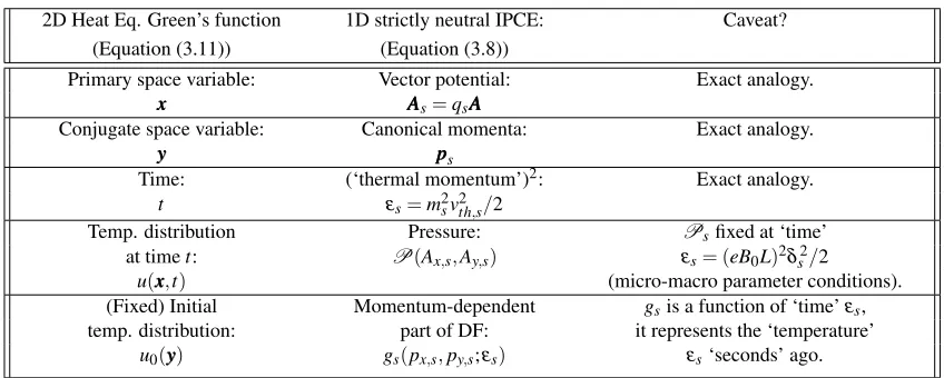
Table 1. The analogy between 1D strictly neutral IPCE and the Green’s function for the 2D heat equation
is the question we consider. Tackling this inverse problem, in the context of equation (3.8), is perhaps the main mathematical challenge for validity of solutions obtained in IPCE, and is akin to going backwards in time (see Evans (2010) for a brief discussion on ‘backwards solutions of the heat equation’). Our known and non-negative ‘present distribution’ is defined byP(Ax,s,Ay,s), and the ‘past distribution’, with questionable sign, is defined bygs(px,s,py,s;εs).
3.4 Implications and interpretation for IPCE
Equation (3.8) casts the inverse problem in direct comparison with the Weiertrass transform, thus making a correspondence between space and time in the heat equation,(x,t), to(AAA,εs)in our inverse problem. However, one difference is that thegs function must - at least parametrically - depend on ‘time’,εs, in contrast to the initial condition (i.e. a time-independent function) that is part of the integrand in Equation (3.10). We know thatgsmust depend onεs, since the result of the integral (the LHS) must be independent ofεs, as mentioned in Section 3.1. Hence, it is not immediately clear how ‘far’ the analogy applies, e.g. is there a differential equation (the heat equation or similar) thatgsand/orPzzobey?
On this subject, and in contrast to the IVP, the approach of IPCE casts the Pzz function as the given/fixed quantity, i.e. thefinal condition. In tackling IPCE, we look for non-negative‘initial condi-tions’,gs, that will produce the correctPzz. Hence, it is reasonable that the ‘initial condition’ should be ‘time-dependent’. That is to say,“given a Pzz(Ax,Ay)function, we calculate the self-consistent gs func-tion ‘εsseconds ago’ by inverting equation (3.8), the integral transform that ‘evolves’ the gs(px,s,py,s;εs) function by ‘εsseconds’ ”. We summarise the analogy between 1D strictly neutral IPCE, and the 2D Green’s function solution of the Heat equation in Table 1.
microscopic parametersmsandvth,s( ˜ppps=ppps/(msvth,s) =ppps/( √
2εs)). Whenever we solve the Vlasov-Maxwell system, much of the hard work is in actually fixing all of the micro-macro parameter relation-ships (e.g. see Neukirch et al. (2009); Wilson & Neukirch (2011); Kolotkov et al. (2015); Allanson et al. (2015, 2017); Wilson et al. (2017); Neukirch et al. (2018) for practical examples). For given values of the macroscopic parameters (B0,L), the one parameter than characterises the micro-macro parameter relationships is
δs= rL,s
L =
msvth,s eB0L
,
forethe fundamental charge. δs is the dimensionless and species-dependentmagnetisation parameter (e.g. see Fitzpatrick (2014)). It is the ratio of the thermal Larmor radius,rLs=vth,s/|Ωs|, to the char-acteristic length scale of the system,L(the gyrofrequency of particle speciessisΩs=qsB0/ms). By fixingδswe also fixεs, according to
m2sv2th,s
2 =:
!
εs:=
(eB0L)2δ2 s
2 , (3.12)
which is analogous to fixing the ‘time’ in the heat equation analogy.
3.5 Using Fourier transforms to solve IPCE
As written, Equation (3.8) definesP(Ax,s,Ay,s)as a 2Dconvolutionof the functionsGs=e−(p 2
x,s+p2y,s)/4εs
andgs(px,s,py,s)] As such, and using the convolution theorem,gscan - at least formally - be written gs(pxs,pys;εs) =4π εsIFTP˜zz/G˜s, (3.13) for IFT the 2D inverse Fourier transform, and ˜Pzz, ˜Gsdenoting the 2D Fourier transforms ofPzzandGs respectively. This Fourier transform method has been used by authors to solve IPCE (e.g. see Channell (1976); Harrison & Neukirch (2009a). Indeed, at first glance, it would seem that using equation (3.13) is the general solution to our IPCE problem. However, the solution defined is only formal, without further investigation. It is not of use when either the Fourier transform of thegsorPfunctions cannot be evaluated, or when the inverse Fourier transform expression on the RHS of equation (3.13) cannot be evaluated. It may be the case that these transforms cannot be evaluated either in the sense that there exists no exact analytic answer in closed form, or that they are divergent (e.g. see Channell (1976); Allanson et al. (2016) for examples and discussion).
The subsequent work in this paper makes use of, and develops, the theory of solutions to IPCE with the use of Hermite polynomial expansions. This technique is to be seen as an alternative method to Fourier transforms.
3.6 Summary
4. Expansions in Hermite polynomials
4.1 Hermite polynomials
The use of Hermite polynomials in kinetic theory dates back, at least, to Grad (1949b) in the study of rarefied collisional gases, in which non-equilibrium DFs are represented by shifted Maxwellians multiplied by an expansion in “n-dimensional” Hermite polynomials (Grad, 1949a). However, the most typical approach in collisionless and weakly collisional plasma kinetic theory is to use expansions in ‘scalar’ Hermite polynomials (Zayed, 1996), defined by
Hn(p) = (−1)nep 2 dn
d pne
−p2
, (4.1)
Z ∞
−∞Hm(p)Hn(p)e −p2
d p = δm,n2nn! √
π, (4.2)
forδm,nthe Kronecker delta, and p∈R. Hermite polynomials are a complete orthogonal set of
poly-nomials forg(p)∈L2(R,e−p2d p)(Sansone, 1959; Arfken & Weber, 2001). That is to say that for any
piecewise continuousg(p), such that
Z ∞
−∞
|g(p)|2e−p2d p<
∞, (4.3)
then there exists an (infinite) expansion in Hermite polynomials,∑∞n=0cnHn(p), such that
lim k→∞
Z ∞
−∞
g(p)− k
∑
n=0
cnHn(p) 2
e−p2d p=0. (4.4)
Hermite polynomials have a long history in kinetic theory precisely due to equation (4.2): they are a natural orthogonal basis with which to use when also considering Gaussian/Maxwellian/normal profiles ∼e−p˜2 ∼e−v˜2, for some appropriately normalised momenta or velocity ( ˜por ˜v).
4.2 Hermite polynomials for exact VM equilibria
In the work by Abraham-Shrauner (1968), expansions in Hermite polynomials of the canonical momen-tum are used to solve the VM system for the case of ‘stationary waves’ in a manner similar to that to be described in this section. In the laboratory frame, these nonlinear waves are not Vlasov equilibria, however they are equivalent to Vlasov equilibria once a transformation is made to a frame co-moving with the wave. Abraham-Shrauner considers a 1D plasma with only one component of current density, first in a general sense, and then considers three different magnetic field configurations. Alpers (1969) also presents a somewhat general discussion on the use of Hermite polynomials for 1D VM equilibria, and proceeds to consider models suitable for the magnetopause, with both one component of the current density, and with two. In the work by Channell (1976), two methods are presented for the solution of the inverse problem with neutral VM equilibria, by means of example. These two methods are inversion by Fourier transforms and – once again – expansion over Hermite polynomials respectively. Channell uses Hermite polynomials in the canonical momenta, but this time with two components of the current density, for the specific case of a magnetic field that is especially suitable to be considered as a stationary wave solution.
use Hermite polynomial expansions in velocity space, for 1D and 2D plasmas respectively. Hewett et al. (1976) assume a representation for the DF using expansions in velocity space, but with only one current density component, and ensure self-consistency with Maxwell’s equations numerically, whereas Suzuki & Shigeyama (2008) use an analytical approach, e.g. demonstrating that the Hermite polynomial approach can reproduce known equilibria such as the Harris sheet (Harris, 1962), and the Bennett Pinch (Bennett, 1934).
Crucially, none of the above references sytematically tackled the necessary mathematical conditions of convergence and non-negativity in a rigorous way. Motivated by new exact Vlasov-Maxwell solu-tions involving expansions in Hermite polynomials in Allanson et al. (2015), the work in Allanson et al. (2016) formally treated the use of Hermite polynomials in IPCE, and tackled the problems of conver-gence, boundedness and non-negativity of the resultant DF. This work will be discussed, and built upon, in the following sections.
To give a subset of (modern) examples outside the realm of equilibrium studiesper se, Hermite polynomial expansions are used by Daughton (1999) to assess the linear stability of a Harris current sheet; by Camporeale et al. (2006) also on the linear stability problem, using a truncation method some-what like that of Grad (1949b), and managing to bypass the traditional approach of integrating over the ‘unperturbed orbits’ (Coppi et al., 1966; Drake & Lee, 1977; Quest & Coroniti, 1981; Daughton, 1999); by Zocco (2015) on linear collisionless Landau damping (Landau, 1946; Mouhot & Villani, 2011); by Schekochihin et al. (2016); Adkins & Schekochihin (2018) on the problem of the free-energy associ-ated with velocity-space moments of the DF, in the context of plasma turbulence; and by Servidio et al. (2017) in the analysis of the plasma velocity-space cascade observed by the MMS mission in the Earth’s magnetosheath.
4.3 Formal solutions to 1D IPCE using Hermite polynomials
Whereas Equations (4.1) and (4.3) are the standard ‘physicists’ definitions of Hermite polynomials, it will be of use in this work, as in Alpers (1969); Channell (1976); Allanson et al. (2015, 2016) to consider the scaled functionHn(p/(2√εs)). This slight modification results in changes to Equations (4.1), (4.2), (4.3) and (4.4), easily achieved by substitution.
In fact, we see that expansions in Hermite polynomialsHn(p/(2 √
εs))are a complete orthogonal set for f ∈L2(R,e−p2/(4εs)d p). By equation (4.3), we see that this means that expansions in Hermite
polynomials,Hn(p/(2√εs)), are valid representations for piecewise-continuous functionsg, such that |g|6Mep2/(8εs), forM<∞. This condition is more strict than that for the existence of the integrals in
equations (3.8) and (3.10), i.e. the validity of the Weierstrass transform representation (equivalent to |g|6Mep2/(4εs)).
Expansions in Hermite polynmials are of particular interest when the Fourier transform inversion technique detailed in Section (3.5) is intractable, and/or whenPzz(Ax,Ay)is not given in closed form. In Allanson et al. (2016), IPCE was solved using Hermite polynomial expansion, and the assumption was made that the Maclaurin expansion ofPzz(Ax,Ay)was either ‘summatively’ or ‘multiplicatively’ separable in it’s indices, i.e. of the form
Pzz∝P1(Ax) +P2(Ay), or Pzz∝P1(Ax)P2(Ay). (4.5)
suppose thatPzz(Ax,Ay)is given as a 2D sum of the most general form,
Pzz(Ax,Ay) =n0
βe+βi
βeβi
∑
m,n cm,nAx B0L
m A y B0L
n
, (4.6)
with the RHS a convergent Maclaurin expansion with infinite radius of convergence in both of its arguments. The indices m,n∈ {0,1,2, ...}, and the coefficient cm,n∈R. (Note that convergence of
the Maclaurin expansion of Pzz, and hence the convergence of the sum of derivatives, implies that Pzz∈C∞(R2), e.g. see Bartle & Sherbert (2000)).
Using theory as in Bilodeau (1962); Allanson et al. (2016), it can be shown that the following expansion in Hermite polynomials
gs(px,s,py,s;εs) =
∑
m,ncm,nsgn(qs)m+n
δs √
2 m+n
Hm
px,s 2√εs
Hn
p y,s 2√εs
, (4.7)
is, formally speaking, an exact inverse solution of equation (3.7), forPzzgiven by equation (4.6). The only change in this calculation, as compared to those thoroughly detailed in Allanson et al. (2015, 2016), is that the once ‘separable’ indexcm,n(i.e.‘additively’ separable,cm,n=am+bn; or ‘multiplicatively’ separable,cm,n=ambn), is now not assumed to be separable. However, this constant index/coefficient falls outside of any integrals, and has no effect on the main outcome.
4.4 Mathematical criteria
Since ags function found using the Hermite polynomial method - as in equation (4.7) - could be an infinite series of polynomials that does not represent a known function in closed form, it is by no means clear ifgsis everywhere non-negative. This issue is recognised by Abraham-Shrauner (1968); Hewett et al. (1976). Not only is the non-negativity in question, but it is not obvious whether a given expansion in Hermite polynomials even converges, and this question was also raised by Hewett et al. (1976). Finally, even if the Hermite expansion converges, it must -when multiplied by the Maxwellian factor (equation (3.1)) - produce a DF for which velocity moments of all order exist, as discussed in Section 2. In order to have full confidence in the Hermite polynomial method we need to address these issues of non-negativity, convergence, and the existence of moments.
We should mention that thereversequestions are well established, i.e. if onea prioriknows the DF in closed form, or at least if Equation (4.3) is satisfied. In such circumstances, one can represent a given non-negative DF as a Maxwellian multiplied by an expansion in Hermite polynomials,Hn(p/(2
√
εs)), provided thegsfunction grows at a rate belowep
2/(8ε
s)∼ev2/4v2th,s (Grad, 1949b; Widder, 1951).
In Allanson et al. (2016), sufficient conditions on the cm,n coefficients were found that when sat-isfied, guaranteed the convergence of the Hermite expansion in the case of additive or multiplicative separability. The resultant DFs were also demonstrated to be bounded over all velocity/momentum space. Furthermore, it was proven for certaingsfunction classes that the derived Hermite polynomial expansion will correspond to a non-negative DF, for at least some finite range of values of 0<δs<δc,s.
4.5 Convergence for separable indices
the corresponding Hermite expansions of the form
gjs(pjs;εs) =
∞
∑
m=0
amsgn(qs)m δs √ 2 m Hm p js 2√εs
(4.8)
for j=x,y, converge for allpjs, provided
lim m→∞ √ m am+1 am
<1/δs, (4.9)
in the case of a series composed of both even- and odd-order terms, or
lim m→∞m
a2m+2 a2m
<1/(2δs2), lim m→∞m
a2m+3 a2m+1
<1/(2δs2), (4.10)
in the case of a series composed only of even-, or odd-order terms, respectively. In order to get a better understanding of the meaning of this theorem, it is instructive to recapitulate the results in a continuous setting. One could imagine the modulus of the coefficients,|am|, as a subset of the range of a continuous function of the independent variablem,
|am|,m=0,1,2, ....
→ a=a(m),m∈[0,∞), s.t. a(0) =|a0|,a(1) =|a1|... . In this case, we require
a(m) =O(au(m)), s.t. au(m) = (δs2m)−m/2,
since the functionaudefines the limiting behaviour ofam, according to the restrictions of Equations (4.9) and (4.10), i.e
au(m+1) au(m)
= 1 δs √ m,
au(2m+2)
au(2m)
= 1
2δs2m
,
au(2m+3)
au(2m+1)
= 1
2δs2m.
Hence the modulus of the coefficients, |am| must ‘fall below’ the graph of (δs2m)−m/2 for largem, depicted in Figure 1.
4.6 Convergence for non-separable indices
Here we generalise the results of Allanson et al. (2016), as detailed in Section 4.5, for the convergence of a Hermite expansion representation for gs that is indexed by a non-separable index, cm,n(i.e. the general solution that corresponds to the pressure function in equation (4.6)).
FIG. 1. If the modulus of the coefficients,|am|, ‘fall below’ the graph of(δs2m)−m/2asm→∞, then the Hermite series will
converge.
indexed by the 2D indexcm,n, is the IPCE solution forPzzdefined by equation (4.6). Now, letdmanden be 1D indices fixed by the following conditions,
dm∈D := n
|cm,n?|: lim
m→∞|cm+1,n?/cm,n?|=maxn
lim
m→∞|cm+1,n/cm,n|
,m=0,1,2, ...o,(4.11) en∈E :=
n
|cm?,n|: lim
n→∞|cm?,n+1/cm?,n|=maxm
lim
n→∞|cm,n+1/cm,n|
,n=0,1,2, ..o. (4.12) Inrow−columnmatrix terminology, that is to say that dm is a 1D index that identifies the (not nec-essarily unique) column,n=n?, for which thecm,nindices decay most slowly asm→∞. Likewise, enidentify the (not necessarily unique) row,m=m?, for which thecm,nindices decay most slowly as n→∞.
Oncedmandenare identified, we can - for sufficently largemandn- formally bound the summand of the general solution (equation (4.7)),
cm,nsgn(qs)m+n δs √ 2 m+n Hm
px,s 2√εs
Hn
py,s 2√εs
<dmen δs √ 2 m+n Hm
px,s 2√εs
Hn
py,s 2√εs
,
and construct a sum composed of these upper bounds, according to
gs,bound=
∞
∑
m=0 ∞∑
n=0 dmenδs √ 2 m+n Hm
px,s 2√εs
Hn
py,s 2√εs
. (4.13)
The RHS of this equation is now of separable form. If each individual sum (over bothm andn) is convergent, then the expression on the RHS is convergent. Then, by using the comparison test (e.g. see Bartle & Sherbert (2000)), convergence of the 2D series,gs,upper, guarantees convergence of the series representation ofgsin equation (4.7).
One can now treat equation (4.13) in the same manner as in Allanson et al. (2016), and derive conditions on thedm andencoefficients for convergence of the general solution, exactly analogous to those of equations (4.9) and (4.10), and by using an upper bound on Hermite polynomials (e.g. see Sansone (1959))
|Hj(x)|<k p
As a result, a sufficient condition for the Hermite series representation ofgsin equation (4.7) to converge is given by
lim m→∞ √ m dm+1 dm
<1/δs,
in the case of a series composed of both even- and odd-order terms, or
lim m→∞m
d2m+2 d2m
<1/(2δs2), lim m→∞m
d2m+3 d2m+1
<1/(2δs2),
and analogously foren, withdmandendefined by equations (4.11) and (4.12).
4.7 The existence of all velocity moments
Once the convergence of the Hermite polynomial expansion is established, then one can begin to con-sider the boundedness of the DF, and the existence of velocity moments. In Allanson et al. (2016), it was shown that DFs of the form in equation (4.7) were bounded over all velocity space, but this does not guarantee that the DF has velocity space moments of all orders. For the DF to be physically meaningful, equation (2.3) must be satisfied.
If the Hermite representation ofgsis a convergent series, then by using Equation (4.14) we deduce that
|gs(px,s,py,s;εs)|<Lx,s(εs)Ly,s(εs)exp p2
x,s+p2y,s 8εs2
!
∀px,s,py,s
and forLx,s(εs),Ly,s(εs)finite positive constants, independent of space and momentum, but dependent onεs. Now, by using the form of the DF from equation (3.1) we see that
|fs|<n0 m
s
π
√ 8εs
3/2
Lxs(εs)Lys(εs)ep 2
xs/(8εs2)ep2ys/(8εs2)
×exp
−(pxs−qsAx)2/(4εs2)−(pys−qsAy)2/(4εs2)−v2z/(2v2th,s)
, (4.15)
and we see that boundedness in momentum space (and hence velocity space) is guaranteed. The reason-ing is as follows. Sincepjs=msvj+qsAj, the arguments of the exponentials scale like
exp − v
2 j 4v2th,s
!
, (4.16)
invj velocity space. There is also a spatial dependence in the argument of the exponential, through Aj(z), but this does not affect the value of fsat a givenzvalue. The scaling described by Expression (4.16) not only ensures boundedness, but guarantees that velocity moments of all order exist, since
Z ∞ −∞
vke−v2/(4v2th,s)dv
<∞∀k∈0,1,2, ...
4.8 Non-negativity of the Hermite polynomial solution
The sign of the DF as written in equation (3.1) is identified with the sign ofgs, and hence non-negativity of the DF depends entirely on the non-negativity of thegsfunction. It was demonstrated in e.g. Channell (1976); Allanson et al. (2016), that the non-negativity of thePzzfunction does not necessarily guarantee non-negativity of thegs function. For example, consider the pressure function originally studied by Channell (1976),
Pzz∝1
2 a0+a2
Ax B0L
2!
+1
2 a0+a2
Ay B0L
2!
,
witha0,a2>0. This pressure function is positive for all (Ax,Ay). However, the corresponding gs function is of the form
gs∝1 2
" a0+a2
δs √ 2 2 H2 p xs 2√εs
#
+1
2 "
a0+a2 δs √ 2 2 H2 p ys 2√εs
#
.
By substitutingpxs=pys=0, we see that positivity ofgsis – for given values ofa0anda2– dependent on the size ofεs,
gs(0,0) =a0−a2δs2,
∴gs(0,0)>0 =⇒ δs26 a0 a2
.
The dependence of the sign ofgsonδs, seems to be a rather general principle. In Allanson et al. (2016) it was proven that for a smoothPzzfunction (either summatively or multiplicatively separable), and under thea prioriassumption of a continuousgsfunction that is uniformly bounded from below in momentum space, the correspondinggsfunction is non-negative for at least a finite range ofδsvalues, i.e. for all
δs6δc,s, forδc,s∈(0,∞)some critical value ofδs, and as yet undetermined. Here we generalise this result for the arbitrarily indexed general solution of the form in equation (4.7)
4.9 The limit asδs→0, B0L→∞and fixedεs
First suppose that for a given value ofδs, that there exists some regions in(px,s,py,s)space wheregs<0. Then, the prioriassumption thatgsis uniformly bounded from below, combined with the expression in Equation (4.7) implies that thegsfunction is bounded below according to
gs(px,s,py,s;εs)>c0,0+δsM withM a finite constant,
M =√1
2(pxinf,s,py,s) ∞
∑
n=1 ∞∑
m=1cm,nsgn(qs)m+n
δs √
2 m+n−1
Hm
px,s 2√εs
Hn
py,s 2√εs
,
i.e. the greatest lower bound of all terms ingsabove zeroth order. In Allanson et al. (2016), the next step in the (similar) argument was to letδs→0, independently ofεs(from equation (3.12), we see that this is equivalent to sendingB0L→∞). We see that by lettingδs→0 whilst keepingεs fixed, thatδsM →0, and so
lim δs→0
gs=c0,0= lim B0L→∞
Pzz>0, for fixedεs>0,
sincePzz>0∀(Ax,Ay). Therefore, there must exist some critical value ofδs =δs,c, such that for all
δs<δc,gsis non-negative. Note that if the negative patches ofgjsdo not exist for anyδs, then trivially
5. Discussion & Conclusions
This paper has introduced and reviewed the theory first of collisionless plasma equilibria (Vlasov-Maxwell equilibria), and then of the inverse problem in collisionless plasma equilibria (IPCE) in a general sense. Then we have applied this theory to equlibrium distribution functions that are single valued functions of the constants of motion, and are self-consistent with spatially one-dimensional and strictly neutral magnetised plasmas. We have demonstrated that in this context, IPCE can reduce to the inversion of Weierstrass transforms, and discussed the parallels between IPCE and ‘backwards solutions of the heat equation’. It will be a very interesting topic for future investigation to see if this analogy can bring further useful insight and results.
The main theoretical developments of this paper have focussed on the mathematical criteria that a candidate solution of IPCE must satisfy, and in particular for those solutions obtained by use of a Her-mite polynomial expansion. We have reviewed the recent works by Allanson et al. (2015, 2016) on this topic and placed them in context with existing works using Hermite polynomials in Vlasov-Maxwell equilibria. We have derived new results relating to convergence and non-negativity of a candidate solu-tion for IPCE, as well as the existence of velocity moments of all orders, for distribusolu-tion funcsolu-tions that are consistent with an arbitrarily indexed 2D Maclaurin expansion of the pressure function. In partic-ular, we have proven that non-negative solutions of IPCE will exist over all momentum space, and for some sections of parameter space, for candidate solutions belonging to a certain class. Future work should focus on extending the results regarding non-negativity to a broader class of solutions, since at present we havea priori assumed that the momentum-dependent part of the naive/formal solution to IPCE (thegs function) is uniformly bounded from below, over all parameter and momentum space. It would be useful to understand to what extent this condition can be relaxed, and whether the aforemen-tioned analogy with the heat equation can be brought to bear on this problem. Furthermore, we would like to establish precisely over which values of parameter space the candidate solution is non-negative, i.e. extend the results from being purelyexistenceresults, to something more concrete.
The other obvious generalisation is to relax earlier assumptions relating to the macroscopic nature of the plasma. For example, to what extent does IPCE change when applied to spatially 2D plasmas, non-strictly-neutral or even non-neutral, non-planar (e.g. cylindrical) geometries, or even the inclusion of gravitational effects? Future work could be directed in these directions, motivated by the many possible applications in plasma physics.
Acknowledgment
OA gratefully acknowledges the financial support of the Science and Technology Facilities Council Consolidated Grant Nos. ST/K000950/1 and ST/N000609/1, the Science and Technology Facilities Council Doctoral Training Grant No. ST/K502327/1, and the Natural Environment Research Council Grant No. NE/P017274/1 (Rad-Sat). ST gratefully acknowledges the financial support of Engineering and Physical Sciences Research Council Doctoral Training Grant No. EP/K503162/1, Natural Sciences and Engineering Research Council of Canada Grant Nos. 2016-03719 and RGPIN-2014-03154, and the Faculty of Mathematics, University of Waterloo.
REFERENCES
Abraham-Shrauner, B. (1968) Exact, Stationary Wave Solutions of the Nonlinear Vlasov Equation. Physics of Fluids,11, 1162–1167.
Abraham-Shrauner, B. (2013) Force-free Jacobian equilibria for Vlasov-Maxwell plasmas.Physics of Plasmas,
Adkins, T. & Schekochihin, A. A. (2018) A solvable model of Vlasov-kinetic plasma turbulence in Fourier?Hermite phase space.Journal of Plasma Physics,84(1), 905840107.
Allanson, O., Neukirch, T., Troscheit, S. & Wilson, F. (2016) From one-dimensional fields to Vlasov equilibria: theory and application of Hermite polynomials.Journal of Plasma Physics,82(3), 905820306.
Allanson, O., Neukirch, T., Wilson, F. & Troscheit, S. (2015) An exact collisionless equilibrium for the Force-Free Harris Sheet with low plasma beta.Physics of Plasmas,22(10), 102116.
Allanson, O., Wilson, F., Neukirch, T., Liu, Y.-H. & Hodgson, J. D. B. (2017) Exact Vlasov-Maxwell equilibria for asymmetric current sheets.Geophysical Research Letters,44, 8685–8695.
Alpers, W. (1969) Steady State Charge Neutral Models of the Magnetopause.Astrophysics and Space Science,5, 425–437.
Arfken, G. B. & Weber, H. J. (2001)Mathematical methods for physicists. Harcourt/Academic Press, Burlington, MA, fifth edition.
Attico, N. & Pegoraro, F. (1999) Periodic equilibria of the Vlasov-Maxwell system.Physics of Plasmas,6, 767–770. Aunai, N., Hesse, M., Zenitani, S., Kuznetsova, M., Black, C., Evans, R. & Smets, R. (2013) Comparison between hybrid and fully kinetic models of asymmetric magnetic reconnection: Coplanar and guide field configurations. Physics of Plasmas,20(2), 022902.
Bartle, R. & Sherbert, D. (2000)Introduction to real analysis. John Wiley & Sons Canada, Limited. Baumjohann, W. & Treumann, R. (1997)Basic Space Plasma Physics. Imperial College Press.
Beidler, M. T. & Cassak, P. A. (2011) Model for Incomplete Reconnection in Sawtooth Crashes.Physical Review Letters,107(25), 255002.
Belmont, G., Aunai, N. & Smets, R. (2012) Kinetic equilibrium for an asymmetric tangential layer.Physics of Plasmas,19(2), 022108.
Belmont, G., Grappin, R., Mottez, F., Pantellini, F. & Pelletier, G. (2013)Collisionless Plasmas in Astrophysics. Wiley.
Bennett, W. H. (1934) Magnetically Self-Focussing Streams.Physical Review,45(12), 890–897.
Bernstein, I. B., Greene, J. M. & Kruskal, M. D. (1957) Exact Nonlinear Plasma Oscillations.Physical Review,
108, 546–550.
Bilodeau, G. G. (1962) The Weierstrass transform and Hermite polynomials.Duke Mathematical Journal,29(2), 293–308.
Birdsall, C. & Langdon, A. (2004)Plasma Physics via Computer Simulation. Series in Plasma Physics and Fluid Dynamics. Taylor & Francis.
Bobrova, N. A., Bulanov, S. V., Sakai, J. I. & Sugiyama, D. (2001) Force-free equilibria and reconnection of the magnetic field lines in collisionless plasma configurations.Physics of Plasmas,8, 759–768.
Bobrova, N. A. & Syrovatskiˇi, S. I. (1979) Violent instability of one-dimensional forceless magnetic field in a rarefied plasma.Soviet Journal of Experimental and Theoretical Physics Letters,30, 535–+.
Burgess, D. & Scholer, M. (2015)Collisionless Shocks in Space Plasmas: Structure and Accelerated Particles. Cambridge Atmospheric and Space Science Series. Cambridge University Press.
Camporeale, E., Delzanno, G. L., Lapenta, G. & Daughton, W. (2006) New approach for the study of linear Vlasov stability of inhomogeneous systems.Physics of Plasmas,13(9), 092110.
Channell, P. J. (1976) Exact Vlasov-Maxwell equilibria with sheared magnetic fields.Physics of Fluids,19, 1541– 1545.
Chen, F. (2015)Introduction to Plasma Physics and Controlled Fusion. Springer International Publishing. Coppi, B., Laval, G. & Pellat, R. (1966) Dynamics of the Geomagnetic Tail.Physical Review Letters,16, 1207–
1210.
Daughton, W. (1999) The unstable eigenmodes of a neutral sheet.Physics of Plasmas,6, 1329–1343.
Dorville, N., Belmont, G., Aunai, N., Dargent, J. & Rezeau, L. (2015) Asymmetric kinetic equilibria: General-ization of the BAS model for rotating magnetic profile and non-zero electric field.Physics of Plasmas,22(9), 092904.
Drake, J. F. & Lee, Y. C. (1977) Kinetic theory of tearing instabilities.Physics of Fluids,20, 1341–1353.
Evans, L. C. (2010)Partial differential equations, volume 19 ofGraduate Studies in Mathematics. American Math-ematical Society, Providence, RI, second edition.
Fitzpatrick, R. (2014)Plasma Physics: An Introduction. CRC Press, Taylor & Francis Group. Freidberg, J. P. (1987)Ideal Magnetohydrodynamics. Plenum Publishing Corportation.
Fruit, G., Louarn, P., Tur, A. & Le Qu´eAu, D. (2002) On the propagation of magnetohydrodynamic perturbations in a Harris-type current sheet 1. Propagation on discrete modes and signal reconstruction.Journal of Geophysical Research (Space Physics),107, SMP 39–1–SMP 39–18.
Fu, W.-Z. & Hau, L.-N. (2005) Vlasov-Maxwell equilibrium solutions for Harris sheet magnetic field with Kappa velocity distribution.Physics of Plasmas,12(7), 070701–+.
Gary, S. (2005)Theory of Space Plasma Microinstabilities. Cambridge Atmospheric and Space Science Series. Cambridge University Press.
Ghosh, A., Janaki, M. S., Dasgupta, B. & Bandyopadhyay, A. (2014) Chaotic magnetic fields in Vlasov-Maxwell equilibria.Chaos,24(1), 013117.
Grad, H. (1949a) Note onN-dimensional Hermite polynomials.Comm. Pure Appl. Math.,2, 325–330. Grad, H. (1949b) On the kinetic theory of rarefied gases.Comm. Pure Appl. Math.,2, 331–407.
Grad, H. (1961) Boundary Layer between a Plasma and a Magnetic Field.Physics of Fluids,4, 1366–1375. Greene, J. M. (1993) One-dimensional Vlasov-Maxwell equilibria.Physics of Fluids B,5, 1715–1722.
Guo, F., Li, H., Daughton, W. & Liu, Y.-H. (2014) Formation of Hard Power Laws in the Energetic Particle Spectra Resulting from Relativistic Magnetic Reconnection.Phys. Rev. Lett.,113, 155005.
Harris, E. G. (1962) On a plasma sheath separating regions of oppositely directed magnetic field.Nuovo Cimento,
23, 115.
Harrison, M. G. & Neukirch, T. (2009a) One-Dimensional Vlasov-Maxwell Equilibrium for the Force-Free Harris Sheet.Physical Review Letters,102(13), 135003–+.
Harrison, M. G. & Neukirch, T. (2009b) Some remarks on one-dimensional force-free Vlasov-Maxwell equilibria. Physics of Plasmas,16(2),
022106–+.
Henon, M. (1982) Vlasov equation.Astronomy and Astrophysics,114, 211.
Hesse, M., Aunai, N., Birn, J., Cassak, P., Denton, R. E., Drake, J. F., Gombosi, T., Hoshino, M., Matthaeus, W., Sibeck, D. & Zenitani, S. (2016) Theory and Modeling for the Magnetospheric Multiscale Mission.Space Science Reviews,199(1), 577–630.
Hesse, M., Aunai, N., Sibeck, D. & Birn, J. (2014) On the electron diffusion region in planar, asymmetric, systems. Geophysical Research Letters,41, 8673–8680.
Hesse, M., Aunai, N., Zenitani, S., Kuznetsova, M. & Birn, J. (2013) Aspects of collisionless magnetic reconnection in asymmetric systems.Physics of Plasmas,20(6).
Hesse, M., Kuznetsova, M., Schindler, K. & Birn, J. (2005) Three-dimensional modeling of electron quasiviscous dissipation in guide-field magnetic reconnection.Physics of Plasmas,12(10), 100704–+.
Hewett, D. W., Nielson, C. W. & Winske, D. (1976) Vlasov confinement equilibria in one dimension.Physics of Fluids,19, 443–449.
Hurley, J. (1963) Analysis of the Transition Region between a Uniform Plasma and its Confining Magnetic Field. II.Physics of Fluids,6, 83–88.
Janaki, M. S. & Dasgupta, B. (2012) Vlasov-Maxwell equilibria: Examples from higher-curl Beltrami magnetic fields.Physics of Plasmas,19(3), 032113.
John, F. (1991)Partial Differential Equations. Applied Mathematical Sciences. Springer New York.
Kocharovsky, V. V., Kocharovsky, V. V. & Martyanov, V. J. (2010) Self-Consistent Current Sheets and Filaments in Relativistic Collisionless Plasma with Arbitrary Energy Distribution of Particles.Physical Review Letters,
104(21), 215002.
Kolotkov, D. Y., Vasko, I. Y. & Nakariakov, V. M. (2015) Kinetic model of force-free current sheets with non-uniform temperature.Physics of Plasmas,22(11), 112902.
Krall, N. A. & Trivelpiece, A. W. (1973)Principles of plasma physics. International Student Edition - International Series in Pure and Applied Physics, Tokyo: McGraw-Hill Kogakusha.
Kulsrud, R. (2005)Plasma Physics for Astrophysics. Plasma Physics for Astrophysics. Princeton University Press. Kulsrud, R. M. (1983)MHD description of plasma. In Handbook of Plasma Physics, Volume 1. Amsterdam:
North-Holland.
Lakhina, G. S. & Schindler, K. (1983) Tearing modes in the magnetopause current sheet.Astrophysics and Space Science,97, 421–426.
Landau, L. (1946) On the vibrations of the electronic plasma.J.Phys.(USSR),10, 25–34.
Landau, L. D. & Lifshitz, E. M. (2013)The Classical Theory of Fields. Course of Theoretical Physics. Elsevier Science.
Lee, L. C. & Kan, J. R. (1979) A unified kinetic model of the tangential magnetopause structure.Journal of Geo-physical Research (Space Physics),84, 6417–6426.
Lerche, I. (1967) On the Boundary Layer between a Warm, Streaming Plasma and a Confined Magnetic Field. Journal of Geophysical Research (Space Physics),72, 5295–+.
Lifshitz, E. & Pitaevski˘ı, L. (1981)Physical kinetics. Course of theoretical physics. Butterworth-Heinemann. Liu, Y.-H. & Hesse, M. (2016) Suppression of collisionless magnetic reconnection in asymmetric current sheets.
Physics of Plasmas,23(6), 060704.
Lynden-Bell, D. (1962) Stellar dynamics: Exact solution of the self-gravitation equation.Monthly Notices of the Royal Astronomical Society,123, 447.
Malakit, K., Shay, M. A., Cassak, P. A. & Bard, C. (2010)
Scaling of asymmetric magnetic reconnection: Kinetic particle-in-cell simulations.Journal of Geophysical Research (Space Physics),115, A10223.
Marsch, E. (2006) Kinetic Physics of the Solar Corona and Solar Wind.Living Reviews in Solar Physics,3(1). Marsch, E. & Goldstein, H. (1983) The effects of Coulomb collisions on solar wind ion velocity distributions.
Journal of Geophysical Research: Space Physics,88(A12), 9933–9940.
Marsh, G. (1996)Force-Free Magnetic Fields: Solutions, Topology and Applications. World Scientific, Singapore. Montgomery, D. & Joyce, G. (1969) Shock-like solutions of the electrostatic Vlasov equation.Journal of Plasma
Physics,3, 1–11.
Moratz, E. & Richter, E. W. (1966)
Elektronen-Geschwindigkeitsverteilungsfunktionen f¨ur kraftfreie bzw. teilweise kraftfreie Magnetfelder. Zeitschrift Naturforschung Teil A,21, 1963.
Mouhot, C. & Villani, C. (2011) On Landau damping.Acta Math.,207(1), 29–201.
Mynick, H. E., Sharp, W. M. & Kaufman, A. N. (1979) Realistic Vlasov slab equilibria with magnetic shear.Physics of Fluids,22, 1478–1484.
Neukirch, T., Wilson, F. & Allanson, O. (2018) Collisionless current sheet equilibria.Plasma Physics and Con-trolled Fusion,60(1), 014008.
Neukirch, T., Wilson, F. & Harrison, M. G. (2009) A detailed investigation of the properties of a Vlasov-Maxwell equilibrium for the force-free Harris sheet.Physics of Plasmas,16(12), 122102.
Nicholson, R. B. (1963) Solution of the Vlasov Equations for a Plasma in an Externally Uniform Magnetic Field. Physics of Fluids,6, 1581–1586.
Panov, E. V., Artemyev, A. V., Nakamura, R. & Baumjohann, W. (2011) Two types of tangential magnetopause cur-rent sheets: Cluster observations and theory.Journal of Geophysical Research (Space Physics),116, A12204. Pegoraro, F., Califano, F., Manfredi, G. & Morrison, P. J. (2015) Theory and applications of the Vlasov equation.
European Physical Journal D,69, 68.
Pritchett, P. L. (2008) Collisionless magnetic reconnection in an asymmetric current sheet.Journal of Geophysical Research (Space Physics),113, A06210.
Quest, K. B. & Coroniti, F. V. (1981) Linear theory of tearing in a high-beta plasma.Journal of Geophysical Research,86, 3299–3305.
Sansone, G. (1959)Orthogonal functions. Revised English ed. Translated from the Italian by A. H. Diamond; with a foreword by E. Hille. Pure and Applied Mathematics, Vol. IX. Interscience Publishers, Inc., New York; Interscience Publishers, Ltd., London.
Sauvigny, F. (2012) Partial Differential Equations 1: Foundations and Integral Representations. Universitext. Springer London.
Schamel, H. (1971) Stationary solutions of the electrostatic Vlasov equation.Plasma Physics,13, 491–505. Schamel, H. (1972) Non-linear electrostatic plasma waves.Journal of Plasma Physics,7, 1–12.
Schamel, H. (1986) Electron holes, ion holes and double layers. Electrostatic phase space structures in theory and experiment.Physics Reports,140, 161–191.
Schekochihin, A. A., Parker, J. T., Highcock, E. G., Dellar, P. J., Dorland, W. & Hammett, G. W. (2016) Phase mix-ing versus nonlinear advection in drift-kinetic plasma turbulence.Journal of Plasma Physics,82, 905820212 (47 pages).
Schindler, K. (2007)Physics of Space Plasma Activity. Cambridge University Press.
Schmid-Burgk, J. (1965) Zweidimensionale selbstkonsistente L¨osungen der station¨aren Wlassowgleichung f¨ur Zweikomponentplasmen.
Max-Planck-Institut f¨ur Physik und Astrophysik, Master’s thesis.
Servidio, S., Chasapis, A., Matthaeus, W. H., Perrone, D., Valentini, F., Parashar, T. N., Veltri, P., Gershman, D., Russell, C. T., Giles, B., Fuselier, S. A., Phan, T. D. & Burch, J. (2017) Magnetospheric Multiscale Observation of Plasma Velocity-Space Cascade: Hermite Representation and Theory.Phys. Rev. Lett.,119, 205101. Sestero, A. (1964) Structure of Plasma Sheaths.Physics of Fluids,7, 44–51.
Sestero, A. (1965) Charge Separation Effects in the Ferraro-Rosenbluth Cold Plasma Sheath Model.Physics of Fluids,8, 739–744.
Suzuki, A. & Shigeyama, T. (2008) A novel method to construct stationary solutions of the Vlasov-Maxwell system. Physics of Plasmas,15(4), 042107–+.
Swisdak, M., Rogers, B. N., Drake, J. F. & Shay, M. A. (2003) Diamagnetic suppression of component magnetic reconnection at the magnetopause.Journal of Geophysical Research (Space Physics),108, 1218.
Tassi, E., Pegoraro, F. & Cicogna, G. (2008) Solutions and symmetries of force-free magnetic fields.Physics of Plasmas,15(9), 092113–+.
Tasso, H. (1969) Non-linear quasi-neutral electrostatic plasma waves and shock waves.Plasma Physics,11(8), 663. Vasko, I. Y., Artemyev, A. V., Popov, V. Y. & Malova, H. V. (2013) Kinetic models of two-dimensional plane and
axially symmetric current sheets: Group theory approach.Physics of Plasmas,20(2), 022110. Vlasov, A. A. (1968) The vibrational properties of an electron gas.Physics-Uspekhi,10(6), 721–733.
Weinberg, S. (2005)The quantum theory of fields. Vol. I. Cambridge University Press, Cambridge. Foundations. Whipple, E. C., Hill, J. R. & Nichols, J. D. (1984) Magnetopause structure and the question of particle accessibility.
Journal of Geophysical Research: Space Physics,89(A3), 1508–1516.
Widder, D. V. (1951) Necessary and sufficient conditions for the representation of a function by a Weierstrass transform.Transactions of the American Mathematical Society,71, 430–439.
Wilson, F. & Neukirch, T. (2011) A family of one-dimensional Vlasov-Maxwell equilibria for the force-free Harris sheet.Physics of Plasmas,18(8), 082108.
Wilson, F., Neukirch, T. & Allanson, O. (2017) Force-free collisionless current sheet models with non-uniform temperature and density profiles.Physics of Plasmas,24(9), 092105.
Yamada, M., Kulsrud, R. & Ji, H. (2010) Magnetic reconnection.Reviews of Modern Physics,82, 603–664. Yoon, P. H. & Lui, A. T. Y. (2005) A class of exact two-dimensional kinetic current sheet equilibria.Journal of
Geophysical Research (Space Physics),110, 1202–+.
Zayed, A. I. (1996)Handbook of function and generalized function transformations. Mathematical Sciences Refer-ence Series. CRC Press, Boca Raton, FL.
Zelenyi, L. M., Malova, H. V., Artemyev, A. V., Popov, V. Y. & Petrukovich, A. A. (2011) Thin current sheets in collisionless plasma: Equilibrium structure, plasma instabilities, and particle acceleration.Plasma Physics Reports,37(2), 118–160.