Patterson-Sullivan measures
Jonathan M. Fraser
February 15, 2019
Abstract
We consider several (related) notions of geometric regularity in the context of limit sets of geometrically finite Kleinian groups and associated Patterson-Sullivan measures. We begin by computing the upper and lower regularity dimensions of the Patterson-Sullivan measure, which involves controlling the relative measure of concentric balls. We then compute the Assouad and lower dimensions of the limit set, which involves controlling local doubling properties. Unlike the Hausdorff, packing, and box-counting dimensions, we show that the Assouad and lower dimensions are not necessarily given by the Poincar´e exponent.
Mathematics Subject Classification 2010: primary: 30F40, 28A80; secondary: 37F30, 37C45.
Key words and phrases: Kleinian group, Patterson-Sullivan measure, Assouad dimension, regularity dimension.
1
Introduction
1.1 Limit sets of Kleinian groups and the Patterson-Sullivan measure
We consider fractal sets and measures arising from discrete groups of isometries acting on hyperbolic space. For integer d>1, we model (d+ 1)-dimensional hyperbolic space using the Poincar´e ball
Dd+1= n
z∈Rd+1 : |z|<1o
equipped with the hyperbolic metric dH defined by
ds= 2|dz| 1− |z|2.
The boundary at infinity of the space (Dd+1, dH) is S
d =
z∈Rd+1 : |z|= 1 and the
group of isometries is given by the stabliser of Dd+1 in the M¨obius group acting on Rd+1. We denote the group of orientation preserving isometries of (Dd+1, dH) by Con(d), and note that it is isomorphic to the (orientation preserving) M¨obius group acting on Rd. We will sometimes appeal to the upper half-space model of hyperbolic space, where Dd+1 is replaced by Hd+1 = Rd×(0,∞) equipped with the analogous metric, but this is purely for aesthetic reasons as these two models of hyperbolic space are of course isometric and, moreover, there is a M¨obius transformation between the corresponding boundaries which (we will see) preserves all of our notions of dimension. We refer the reader to [B, Ma, K] for a more detailed study of hyperbolic geometry, including the isometry group, and the correspondence between, and equivalence of, the two models we use.
A Kleinian group is a discrete subgroup of Con(d) and such groups act properly dis-continuously on Dd+1 but may fail to act discontinuously on the boundary. The limit set of a Kleinian group Γ is the set of points where the action fails to be discontinuous and it carries a lot of geometric information concerning the group. More precisely, writing
0= (0, . . . ,0)∈Dd+1, the limit set is defined by
L(Γ) = Γ(0)\Γ(0).
This is a compact subset ofSd and often has a beautiful and subtle fractal structure. Note that for definiteness we metrise Sd with the Euclidean metric k · k inherited from Rd+1, although the standard Riemannian metric on Sd is bi-Lipschitz equivalent to this metric and so from a dimension point of view these two natural metrics on the limit set are equivalent.
If the limit set is empty or consists only of one or two points, then the Kleinian group is called elementary and otherwise it is non-elementary, in which case the limit set is nec-essarily uncountable. A Kleinian group is calledgeometrically finite if it has a fundamental domain with finitely many sides. The Poincar´e exponent of a Kleinian group Γ is defined by
δ(Γ) = inf
s >0 : X
g∈Γ
exp(−s dH(0, g(0)))<∞
and plays a central role in the geometry and dimension theory of Γ. In particular, the limit set of a non-elementary geometrically finite Kleinian group has Hausdorff dimension equal to δ(Γ). This important result goes back to the influential papers of Patterson (for Fuchsian groups with some assumptions on parabolic elements) [Pa, Theorems 4.1 and 5.1] and Sullivan (for the general higher dimensional case) [Sul, Theorem 1]. Almost 20 years later it was shown that in this setting the packing and box-counting dimensions of the limit set are also given by δ(Γ). This result is due independently to Bishop and Jones [BJ, Corollary 1.5] and Stratmann and Urba´nski [SU, Theorem 3]. For a review of the Hausdorff, box-counting, and packing dimensions, see [F1, Chapters 2 and 3]. When discussing geometrically finite groups, we will only mention the Hausdorff dimension, which we denote by dimH, since the Hausdorff, packing, and box-counting dimensions coincide in
this case.
Limit sets of non-elementary geometrically finite Kleinian groups are also known to carry an atomless conformal ergodic Borel probability measureµPS of Hausdorff dimension
δ(Γ), known as the Patterson-Sullivan measure. Again, we will only discuss the (lower)
Hausdorff dimension of the Patterson-Sullivan measure, but this is known to equal the
upper packing dimension (indeed, the Patterson-Sullivan measure is exact dimensional, see [SV]). See [F2, Chapter 10] for a review of the dimensions of measures.
Fix a non-elementary geometrically finite Kleinian group and suppose Γ is notparabolic free, that is, it contains at least one parabolic element. LetP ⊆L(Γ) denote the countable set of all parabolic fixed points, that is, points fixed by parabolic elements of Γ. We may fix a standard set of pairwise disjoint horoballs{Hp}p∈P, where eachHpis a horoball with base
point p, that is, a closed Euclidean ball whose interior lies insideDd+1 and is tangent toSd atp. Moreover, the horoballs can be chosen such thatg(Hp) =Hg(p)for allg∈Γ andp∈P.
Thus, although the choice of standard horoballs is not unique, any given choice reflects the geometry of the limit set in a representative way. The stabiliser of a parabolic fixed point p cannot contain hyperbolic or loxodromic elements since if a subgroup of Con(d) contains a parabolic and a hyperbolic/loxodromic element which fix the same point then the group is not discrete. Therefore the parabolic elements in the stabiliser of p in Γ generate a free Abelian group of finite index (as a subgroup of the stabiliser). We define k(p) to be the maximal rank of a free Abelian subgroup of the stabiliser of p in Γ, which is necessarily generated byk(p) parabolic elements all fixingp. For an account of standard horoballs and ranks of parabolic elements, we refer the reader to the opening discussion in [SU]. We note the important fact that δ(Γ)> k(p)/2 for all p∈P.
Givenz∈L(Γ) andt >0, letzt∈Dd+1 be the unique point on the geodesic ray joining
0 to z which is at hyperbolic distance t from 0. WriteS(z, t) ⊂ Sd to denote the shadow
at infinity of thed-dimensional (hyperbolic) hyperplane passing through zt normal to the
geodesic ray joining 0 to z. Basic hyperbolic geometry shows that S(z, t) is a Euclidean ball centred at z with radius uniformly comparable to e−t. The global measure formula states that there is a uniform constant C >1 such that for all z∈ L(Γ) and allt > 0 we have
1
C 6
µPS(S(z, t))
exp(−tδ(Γ)−ρ(z, t)(δ(Γ)−k(z, t))) 6 C (1.1)
where k(z, t) =k(p) if zt∈Hp for somep and 0 otherwise and
ρ(z, t) = inf{dH(zt, y) : y /∈Hp}
if zt ∈ Hp for some p and 0 otherwise. Note that if we choose a different set of standard
horoballs, then the constant C can change and so for definiteness we fix a set of standard horoballs, and therefore a constantC, for the rest of the paper. The global measure formula still holds if Γ is parabolic free and in that case it simplifies to
1
C 6
µPS(S(z, t))
exp(−tδ(Γ)) 6 C. (1.2)
1.2 Regularity dimensions of measures and Assouad dimensions of sets
In this section we work with a general complete metric measure space (X, d, µ) but our results will mostly concern the space (L(Γ),k · k, µPS).
regularity dimensions provide a generally applicable refinement of the notion of Ahlfors-David regularity. Recall that a (non-atomic) measure iss-Ahlfors-David regular if the ratio µ(B(x, R))/Rs is uniformly bounded away from 0 and +∞ for all 0< R6|supp(µ)|. We write supp(µ) ⊆X for the support of µ, |E| for the diameter of non-empty (possibly un-bounded) E ⊆X, and B(x, R) for the open ball of radius R > 0 and centre x ∈X. The
upper regularity dimension ofµ is defined by
dimregµ= inf
(
s>0 : there exists C >0 such that, for all 0< r < R <|supp(µ)|
and all x∈supp(µ), we have µ(B(x, R)) µ(B(x, r)) 6C
R
r s)
and, provided |supp(µ)|>0, the lower regularity dimension ofµ is defined by
dimregµ= sup (
s>0 : there existsC >0 such that, for all 0< r < R <|supp(µ)|
and all x∈supp(µ), we have µ(B(x, R)) µ(B(x, r)) >C
R
r s)
and otherwise it is 0. We adopt the convention that inf∅= +∞. A measureµis doubling if and only if dimregµ <∞, see [JJKRRS, FH2]. Also note that if a set carries an
s-Ahlfors-David regular measure, then the upper and lower regularity dimensions coincide and equal s. The regularity dimensions are heavily related to the Assouad and lower dimensions, which are purely metric notions describing the extremal scaling behaviour of a set in a metric space. These dimensions have fundamental applications in embedding theory and quasi-conformal geometry, for example, and have recently been enjoying a period of intense interest in the fractal geometry literature. We recall the definitions of the Assouad and lower dimensions here, but refer the reader to [R, Fr, L, MT] for more details. For non-emptyE ⊆X andr >0, letNr(E) be the smallest number of open sets with diameter less
than or equal tor required to coverE. TheAssouad dimension of a non-empty setF ⊆X is defined by
dimAF = inf
(
s>0 : there exists C >0 such that, for all 0< r < R <|F|
and all x∈F, we have Nr B(x, R)∩F
6C
R r
s)
and, provided |F|>0, thelower dimension of F is defined by
dimLF = sup
(
s>0 : there exists C >0 such that, for all 0< r < R <|F|
and all x∈F, we have Nr B(x, R)∩F
>C
R r
and otherwise it is 0. It is well-known that for closed F we have
dimLF 6dimHF 6dimAF.
The regularity dimensions can be thought of as the Assouad and lower dimensions of a measure. Indeed, for any Borel probability measure ν fully supported on a closed set F ⊆X, it is easy to see that dimregν 6dimLF 6dimAF 6dimregν but a deeper fact is
that if F is doubling, then
dimAF = inf
dimregν : ν is a Borel probability measure fully supported onF
and
dimLF = sup
dimregν : ν is a Borel probability measure fully supported onF ,
see [KL] and the references therein. Having finite Assouad dimension is equivalent to being doubling, and having strictly positive lower dimension is equivalent to being uniformly perfect. J¨arvi and Vuorinen [JV, Theorem 5.5] proved that limit sets of finitely generated Kleinian groups are uniformly perfect and so it is natural to pursue a quantitative version of this result where one computes the lower dimension explicitly. Indeed, uniform perfectness has been investigated extensively in the context of Kleinian limit sets, see [Su] and the references therein.
We close this section with the observation that the regularity dimensions (and therefore the Assouad and lower dimensions) are preserved under M¨obius transformations. Although simple, this observation is important since properties of the limit set and Patterson-Sullivan measure should be preserved under the action of Con(d) onSd and also should be indepen-dent of the chosen model of hyperbolic space. The observation that the Assouad dimension is preserved under general M¨obius transformations can be found in [L, Theorem A.10] and a similar argument establishes the analogous result for lower dimension. For the action of Con(d) on Sd the situation is already very simple since each element g ∈ Con(d) is bi-Lipschitz on Sd (the bi-Lipschitz constants are not uniform over Con(d), but this does not matter) and so the dimensions of sets and measures supported on Sdare clearly preserved by Con(d). For general M¨obius transformations g : Rd → Rd, if µ is a Borel probabil-ity measure supported on Rd, then, provided µ({g−1(∞)}) = 0, the pushforward measure g(µ) =µ◦g−1 is a Borel probability measure supported onRd and one can show that the regularity dimensions of µand g(µ) coincide. We do not rely on this fact, but point it out to reassure readers that our results are independent of how we model hyperbolic space.
2
Results
Throughout this section Γ<Con(d) will be a non-elementary geometrically finite Kleinian group acting on Dd+1. Also, L(Γ) ⊆Sd will denote the limit set of Γ, µPS the associated
Theorem 2.1. If Γ is a non-elementary geometrically finite Kleinian group which is
parabolic free, then µPS is δ(Γ)-Ahlfors-David regular and therefore
dimAL(Γ) = dimLL(Γ) = dimregµPS= dimregµPS=δ(Γ).
In light of this result, we assume from now on that Γ contains a parabolic element and write 1 6 kmin 6 kmax 6 d to denote the minimal and maximal ranks of parabolic fixed
points, respectively.
Our first result gives precise formulae for the regularity dimensions of the Patterson-Sullivan measure associated with a geometrically finite Kleinian group.
Theorem 2.2. Let Γ < Con(d) be a non-elementary geometrically finite Kleinian group which is not parabolic free. The upper and lower regularity dimensions of the
Patterson-Sullivan measure are continuous and piecewise linear in the Poincar´e exponent both with a
single phase transition at (kmin+kmax)/2. In particular,
dimregµPS = max{kmax,2δ(Γ)−kmin}
and
dimregµPS = min{kmin,2δ(Γ)−kmax}.
We prove Theorem 2.2 in Section 4. We now turn our attention to the related question of the Assouad and lower dimensions and state our main result.
Theorem 2.3. Let Γ < Con(d) be a non-elementary geometrically finite Kleinian group
which is not parabolic free. The Assouad and lower dimensions of L(Γ) are functions of
the Poincar´e exponent of convergence and the maximal and minimal ranks of parabolic fixed
points. In particular,
dimAL(Γ) = max{kmax, δ(Γ)}
and
dimLL(Γ) = min{kmin, δ(Γ)}.
We prove Theorem 2.3 in Section 5. We emphasise here that, even though the Hausdorff, packing and upper and lower box dimensions of L(Γ) always coincide with the Poincar´e exponent, the Assouad and lower dimensions may not.
2.1 Applications and observations
In this section we discuss several consequences of our results, hopefully demonstrating their relevance in other contexts.
The Patterson-Sullivan measure is ‘uniformly perfect’: It follows from Theo-rem 2.2 that the lower regularity dimension of the Patterson-Sullivan measure for a non-elementary geometrically finite Kleinian group is always strictly positive. This can be viewed as a measure theoretic analogue of the result in [JV, Theorem 5.5] that the support of such measures are uniformly perfect, that is, have strictly positive lower dimension.
porous and if the Assouad dimension is full, then so is the conformal Assouad dimension, that is, the Assouad dimension may not be lowered by quasi-symmetric transformations, see [FY, MT]. Theorem 2.3, combined with the deep result of Tukia [T, Theorem D] that δ(Γ)< dif and only if the limit set is not the entire boundary, provides the following precise characterisation of when the Assouad dimension of L(Γ) has full Assouad dimension.
Corollary 2.4. IfΓ<Con(d) is geometrically finite andL(Γ)6=Sd, then the following are
equivalent:
1. the limit set has full Assouad dimension, that is dimAL(Γ) =d,
2. there exists a cusp of maximal rank, that is kmax=d,
3. for any quasi-symmetric transformationφ, we have dimAφ(L(Γ)) =d,
4. the limit set is non-porous.
In fact our arguments prove that the conformal Assouad dimension is always bounded below by kmax and is equal tokmax whenever δ(Γ)6kmax.
Invariant measures with optimal dimensions: The interplay between dynamically invariant sets and measures is central to the dimension theory of dynamical systems with a natural question being: when does a given invariant set support an (ergodic) invariant measure which realises its dimension? This question can then take on different flavours depending on the dimensions involved. Concerning Hausdorff dimension, ‘realising the dimension’ usually means that the Hausdorff dimension of the measure equals the Hausdorff dimension of the set (a measure of maximal dimension). For Assouad and lower dimension, ‘realising the dimension’ means that the upper/lower regularity dimension of the measure equals the Assouad/lower dimension of the set (a measure of minimal/maximal dimension). It is particularly interesting to us whether or not an invariant measure can simulta-neously realise all three of these dimensions when they are distinct. Previous examples seem to support a negative answer to this question. For example, consider the self-affine carpets of Bedford-McMullen [Be, Mc1], which are invariant under the toral endomorphism (x, y) 7→ (mx, ny). It is well-known that there exists a unique invariant probability mea-sure of maximal Hausdorff dimension, namely the McMullen measure. In the case where the carpet does not have uniform fibres, the Assouad, Hausdorff, and lower dimensions are necessarily distinct, see [Fr, Corollary 2.14]. It follows from [FH2, Theorem 2.6] that the upper and lower regularity dimensions of the McMullen measure are always distinct from the Assouad and lower dimensions of the carpet, provided the very strong separation
con-dition (VSSC) is satisfied and the carpet does not have uniform fibres. There are invariant
measures, introduced in [FH1, Theorem 2.3], which simultaneously realise the Assouad and lower dimensions, provided the VSSC is satisfied. These measures are known ascoordinate
uniform measures, but are necessarily distinct from the McMullen measure and so do not
realise the Hausdorff dimension.
We can provide the first example of a dynamically invariant measure which simultane-ously realises the (distinct) lower, Hausdorff and Assouad dimensions of its support, thus answering the above question in the affirmative. However, as we shall see, this simultaneous realisation is still very rare in this context. Note that µPS always realises the Hausdorff
Corollary 2.5. Let Γ < Con(d) be a non-elementary geometrically finite Kleinian group which is not parabolic free. Then
dimregµPS= dimAL(Γ) ⇔ δ(Γ)6(kmin+kmax)/2
and
dimregµPS= dimLL(Γ) ⇔ δ(Γ)>(kmin+kmax)/2.
Therefore we have
dimregµPS= dimLL(Γ)<dimHµPS= dimHL(Γ)<dimregµPS= dimAL(Γ)
if and only if kmin < kmax andδ(Γ) = (kmin+kmax)/2.
Coming up with an explicit example where kmin < kmax and δ(Γ) = (kmin+kmax)/2 is
not straightforward but can be achieved as a subgroup of Con(2) by starting with a group with cusps of both possible ranks (1 and 2) and smallδ(Γ), i.e. close tokmax/2 = 1. Then
by varying some hyperbolic elements in a region which does not interfere with the cusps one can slowly increase δ(Γ) achievingδ(Γ) = 3/2 at some point by the intermediate value theorem. We do not pursue the details.
Relationships between dimensions: It is a common consideration in dimension theory to identify possible relationships between dimensions in particular contexts, see for example [Fr, Section 4]. A succinct corollary of our main results demonstrates the following precise dichotomy for the dimensions of limit sets of Fuchsian groups, which is somewhat reminiscent of a known dichotomy for the dimensions of self-similar (and self-conformal) sets in R, see [FHOR, Theorem 1.3] and also [AT, Theorems A and B] for the conformal case.
Corollary 2.6. Let Γ < Con(1) ∼= PSL(2,R) be a non-elementary geometrically finite
Fuchsian group with limit set L(Γ)a proper subset of S1.
1. If Γ is parabolic free, then
0<dimLL(Γ) = dimHL(Γ) = dimAL(Γ) =δ(Γ)<1.
2. If Γ contains a parabolic element, then
1/2<dimLL(Γ) = dimHL(Γ) =δ(Γ)<dimAL(Γ) = 1.
We provide one more example, which could be contrasted with, for example, a di-chotomy observed by Mackay [M, Theorem 1.1] and [Fr, Corollary 2.14], which shows that for Bedford-McMullen carpets one either has the Assouad, lower and Hausdorff dimensions all equal or all distinct.
Corollary 2.7. Let Γ < Con(d) be a non-elementary geometrically finite Kleinian group
with at least one cusp, but with uniform cusp ranks, that is kmin =kmax>1. Then either
Relationships with local dimensions: The regularity dimensions are related to the local dimensions. The upper local dimension of a Borel measureµatx∈supp(µ) is defined by
dimloc(µ, x) = lim sup
r→0
logµ(B(x, r)) logr .
The lower local dimension dimloc(µ, x) is defined in a similar way, replacing lim sup with lim inf. It is straightforward to see that for any measure µ
dimregµ6inf
x dimloc(µ, x)6supx dimloc(µ, x)6dimregµ,
see for example [FH2, Theorem 2.1] for the upper regularity dimension case. Moreover, equality between any of the terms above can be interpreted as some form of homogeneity of ν. Such homogeneity is rare for Patterson-Sullivan measures associated to Kleinian groups with parabolic elements.
Proposition 2.8. Let Γ<Con(d)be a non-elementary geometrically finite Kleinian group, which is not parabolic free. Then
sup
z∈L(Γ)
dimloc(µPS, z) = max{δ(Γ),2δ(Γ)−kmin}
and
inf
z∈L(Γ)dimloc(µPS, z) = min{δ(Γ),2δ(Γ)−kmax}.
In particular,
dimregµPS= sup
z∈L(Γ)
dimloc(µPS, z) ⇔ δ(Γ)>(kmin+kmax)/2
and
dimregµPS= inf
z∈L(Γ)dimloc(µPS, z) ⇔ δ(Γ)6(kmin+kmax)/2.
The calculation of the extremal upper and lower dimensions is not new, see for example [S], but we include the explicit calculation for completeness. However, we delay this until Section 6 since it relies on observations we make during the proof sections.
2.2 Examples
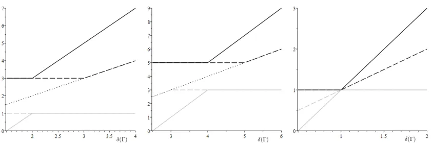
In order to provide a visual picture for the statements of Theorems 2.2 and 2.3, we plot the dimensions in three distinct cases: kmin < kmax/2,kmax/2< kmin < kmax and kmin=kmax.
Figure 1: Three plots showing the dimensions we study as functions of δ(Γ)∈(kmax/2, d].
The regularity dimensions of µPS are plotted with solid lines, the Assouad and lower
di-mensions of L(Γ) are plotted with dashed lines, and δ(Γ) is plotted with a dotted line (for reference). The upper regularity and Assouad dimensions are plotted in black and the lower regularity and lower dimensions are plotted in grey. Left: kmin = 1< kmax= 3 andd= 4.
Centre: kmin= 3< kmax= 5 andd= 6. Right: kmin=kmax= 1 and d= 2.
Also for aesthetic purposes, we close this section by discussing a famous example. The
Apollonian gasket or Apollonian circle packing, see Figure 2, is a well-known geometric
object formed by starting with 4 mutually tangent circles lying in C, one containing the other three, and then inductively adding in circles of the largest possible radius which lie tangent to three previously added circles. See [Po] for an interesting discussion of Apollonian packings ranging from their genesis to problems at the forefront of modern mathematics and [MPR] for more on the visualisation of Apollonian circle packings as well as other Kleinian limit sets. It is well-known that given any two circle packings formed in this way there is a M¨obius transformationg∈PSL(2,C) taking one to the other, that is, there is a unique circle packing up to M¨obius images. Therefore we may talk about the Apollonian circle packing and note that it is the limit set of a geometrically finite Kleinian group Γ<PSL(2,C)∼= Con(2), sometimes known as the Apollonian group.
The parabolic fixed points are the points of mutual tangency between two circles in the packing and it is straightforward to see that the rank of each of these points is 1, and therefore kmin = kmax = 1. Estimating the Poincar´e exponent for this group is
dif-ficult, but has received a lot of attention in the literature and very good bounds are now available. In particular, δ(Γ)≈ 1.305. . ., see [Mc2]. We note that the Poincar´e exponent can also be computed as the circle packing exponent, which is somewhat easier to handle computationally, see [Boy, P]. Therefore
dimregµPS= 2δ(Γ)−1≈1.61. . .
dimregµPS= dimLL(Γ) = 1
Figure 2: An Apollonian circle packing viewed as the limit set of the Apollonian group acting on H3.
2.3 The geometrically infinite case
In this section we briefly discuss the geometrically infinite case. Limit sets of non-elementary geometrically infinite Kleinian groups are not as well-understood as the geometrically finite case. They can also exhibit many different features, not present in the geometrically finite case, for example, one generally has δ(Γ)6dimHL(Γ)6dimBL(Γ), but either or both of
these inequalities can be strict. It was recently shown by Falk and Matsuzaki [FM, Theorem 1] that the (upper) box dimension of the limit set is given by theconvex core entropy,hc(Γ),
see [FM, Definition 3.1]. This result, combined with the observation that our proof of the
lower bound for the Assouad dimension of the limit set does not use geometric finiteness,
yields the following estimate.
Corollary 2.9. If Γ<Con(d) is a non-elementary Kleinian group, then
dimAL(Γ)>max{kmax, hc(Γ)}.
It is natural to ask if equality holds here, but this turns out not to be true in general. We demonstrate this by example at the end of this section.
A weakening of geometric finiteness is the concept of conformal finiteness, introduced by Chang, Qing and Yang [CQY, Definition 3.2], which extends the older notion ofanalytic
finiteness for subgroups of Con(2). In particular, all finitely generated Kleinian groups
Γ < Con(2) are analytically and conformally finite (this is known as Ahlfors finiteness theorem and is known to fail in higher dimensions, see [K]). It is shown in [CQY, Theorem 0.1] that if Γ < Con(d) is conformally finite and dimHL(Γ) < d, then it is geometrically
Corollary 2.10. If Γ < Con(d) is a non-elementary conformally finite Kleinian group, then
dimAL(Γ) = max{kmax,dimHL(Γ)}.
Finally we present a simple example illustrating the wildness of infinitely generated Kleinian groups, see [Mat] for discussion of the Hausdorff dimension. Specifically, for any 0 < α < β < 1, we sketch the construction of an infinitely generated Fuchsian group Γ<PSL(2,R)∼= Con(1) with
dimLL(Γ) = 0<dimHL(Γ)6α < β6dimBL(Γ)<dimAL(Γ) = 1.
Moreover, Γ will be parabolic free and so this shows that the Assouad dimension can be large for reasons other than parabolic points in the infinitely generated case. Of course there is a natural duality between parabolic systems and infinitely generated systems (for example, via ‘inducing schemes’) and so it is really just two sides of the same coin. By the result of Falk and Matsuzaki mentioned above this example also demonstrates that dimAL(Γ)>max{kmax, hc(Γ)}is possible in the infinitely generated case. It also shows that
limit sets of infinitely generated Fuchsian groups need not be uniformly perfect (they can have lower dimension equal to 0). This observation is not new, see for example [Su, Example 7.1]. Finally, this example also demonstrates that for infinitely generated Γ<Con(d), the difference dimAL(Γ)−dimHL(Γ) can approach d, whereas in the geometrically finite case
it can only approachd/2, see Theorem 2.3 noting thatδ(Γ)> kmax/2. In the geometrically
finite case the (potentially) larger difference dimAL(Γ)−dimLL(Γ) is bounded above by
d−1 and this bound is achieved precisely when kmin = 1 < d = kmax, whereas in the
geometrically infinite case it can be d.
Fix 0< α < β <1 and set γ = 1/β−1>0. For integern>1, letxn =xn(γ) = 1/nγ
and 0 < rn = rn(α, γ) < e−n be very small radii, chosen so that the balls B(xn, rn) are
pairwise disjoint. Let gn :H2 → H2 be defined by reflecting in the boundary of the ball B(xn, rn) (an orientation reversing M¨obius transformation). Since the balls B(xn, rn) are
pairwise disjoint the group
Γ0 =hgn : n>1i
is a discrete infinitely generated free group. Moreover, Γ0 has an index 2 subgroup Γ <Γ0 which is a Fuchsian subgroup of PSL(2,R). It is easy to see that
L(Γ)⊆ ∪nB(xn, rn)∪ {0}
and that for all n >1, L(Γ)∩B(xn, rn) 6=∅. By considering the dimensions of the set of
centres {xn}n>1 this is already enough to prove that
dimBL(Γ)>
1 1 +γ =β
and dimAL(Γ) = 1. Moreover, since the radii rn decay exponentially and the gaps
between the balls only decay polynomially, it follows that dimLL(Γ) = 0. Indeed,
Ne−n(B(xn, n−(γ+1))) .1. Finally, dimHL(Γ) can be made arbitrarily small by choosing
the radii rn small enough. With a little more work one can show that the box dimension
is indeed controlled by the box dimension of the set of fixed points of the generators, and therefore is preciselyβ =hc(Γ)<1 = dimAL(Γ). See [MU] for more general settings where
3
Notation and preliminary results
Throughout the rest of the paper we will writeA.B to mean that there exists a universal constantc>1 such thatA6cB. In particular,cis allowed to depend on parameters fixed in the hypotheses of the theorems given above, such as the group Γ, and ambient spatial dimensiond. The constantcisnot allowed to depend on parameters introduced during the proof, most importantly the scales R, r or (logarithmic) scales T, t or on particular points z∈Dd+1∪Sd. We write A&B to mean B .A and A≈B to mean A.B and A&B.
We begin by reformulating the statement of the global measure formula, which also serves as a crucial example using the notation described above. It follows immediately from (1.1) that
µPS(B(z, e−t)) ≈ exp(−tδ(Γ)−ρ(z, t)(δ(Γ)−k(z, t))) (3.1)
for allz∈L(Γ) andt >0 whereB(z, e−t) is the Euclidean ball centred atzwith radiuse−t. Note that the implied constants only depend on the group Γ and the choice of standard horoballs (which we may assume depends on the group). The implied constants do not depend on z ort.
Since the global measure formula is most conveniently expressed in terms of logarithmic scales t >0, that is, balls with radiuse−t, we adopt this convention whenever we use (3.1). In particular, when computing the upper and lower regularity dimensions we will use a ‘large’ scale R =e−t and a ‘small’ scale r = e−T forT > t > 0. Therefore to prove that dimregµPS6α, say, it suffices to prove that
µPS(B(z, e−t))
µPS(B(z, e−T)) .
e−t e−T
α
for all z ∈ L(Γ) and T > t > 0, whereas to prove that dimregµPS > β, say, it suffices to
prove that
µPS(B(z, e−t))
µPS(B(z, e−T)) &
e−t e−T
β
for infinitely many z∈L(Γ) andT > t >0 with T−t→ ∞.
We may assume without loss of generality that 0 ∈/ Hp for all p, which means that
ρ(z, t) 6 dH(zt,0) 6 t for all z ∈ L(Γ) and t > 0. The rest of this section is devoted to
establishing simple estimates for the ‘escape functions’ρ(z, t), which will be used throughout the rest of the paper.
Lemma 3.1 (Quick escape lemma). Let t1, t2 >0 and z ∈L(Γ). Ifzt1 and zt2 do not lie
in a common standard horoball, then
ρ(z, t1) +ρ(z, t2) 6 |t1−t2|
and if zt1 and zt2 do lie in a common standard horoball, then
|ρ(z, t1)−ρ(z, t2)| 6 |t1−t2|.
Proof. If zt1 and zt2 do not lie in the same horoball, then we can find t0 lying between t1
and t2 such thatzt0 does not lie in the interior of any horoball. It follows that
= |dH(zt1,0)−dH(0, zt2)|
= |t1−t2|
since 0, zt1, zt2, zt0 lie on the same geodesic.
Now supposezt1, zt2 ∈Hp for some standard horoball Hp. Then zt1 can escape Hp by first going to zt2 and then escaping from there via the most efficient route. Therefore
ρ(z, t1)6dH(zt1, zt2) +ρ(z, t2) =|t1−t2|+ρ(z, t2)
and the result follows by symmetry.
Lemma 3.2 (Parabolic centre lemma). Suppose p is a parabolic fixed point associated to
a standard horoball Hp. Then ρ(p, t) ∼t as t → ∞ and for all sufficiently large t > 0 we
have k(p, t) =k(p).
Proof. Let s > 0 be such that ps is the point of intersection of the ray joining 0 and p
with the boundary of the horoball Hp. It follows thatpt ∈Hp ⇔ t>s and therefore for
t >s, we have k(p, t) = k(p). Moreover, since the geodesic joining pt and ps is normal to
the boundary of Hp,
1> ρ(p, t)
t =
dH(pt, ps)
t =
t−s
t →1
as t→ ∞, as required.
We will also need a version of Lemma 3.1 for when the point z is not fixed. We state and prove this version separately for clarity.
Lemma 3.3 (Quick escape lemma II). Let T > t >0 and x, y∈L(Γ) with kx−yk.e−t.
If xt and yT do not lie in a common standard horoball, then
ρ(x, t) +ρ(y, T) . T−t
and if xt andyT do lie in a common standard horoball, then
|ρ(x, t)−ρ(y, T)| . T −t.
Proof. Suppose that xt and yT do not lie in a common standard horoball and assume
without loss of generality that at least one of xt, yT lies in the interior of some horoball.
Therefore there must be a point on the geodesic joiningxtandyT which lies on the boundary
of this horoball. It follows that
ρ(x, t) +ρ(y, T) 6 2dH(xt, yT) 6 2 (dH(xt, xT) +dH(xT, yT))
. T −t+ arcsinh k
x−yk
e−T
. T −t+ arcsinh
e−t e−T
as required.
Now supposext and yT do lie in a common standard horoball. Then, combining ideas
from the proof of Lemma 3.1 and the above argument, we get
|ρ(x, t)−ρ(y, T)| 6 dH(xt, yT) 6 dH(xt, xT) +dH(xT, yT) . T −t
completing the proof.
4
The regularity dimensions of
µ
PS: proof of Theorem 2.2
4.1 The upper regularity dimension
4.1.1 Upper bound: dimregµPS6max{kmax,2δ(Γ)−kmin}
Let z∈L(Γ) andT >t >0. It follows from (3.1) that
µPS(B(z, e−t))
µPS(B(z, e−T)) .
exp(−tδ(Γ)−ρ(z, t)(δ(Γ)−k(z, t))) exp(−T δ(Γ)−ρ(z, T)(δ(Γ)−k(z, T)))
=
e−t e−T
δ(Γ)
exp(ρ(z, t)(k(z, t)−δ(Γ)))
exp(ρ(z, T)(k(z, T)−δ(Γ))) (†)
If zt and zT lie in the same standard horoballHp, then, continuing from (†), we get
µPS(B(z, e−t))
µPS(B(z, e−T)) .
e−t e−T
δ(Γ)
exp(ρ(z, t)(k(p)−δ(Γ))) exp(ρ(z, T)(k(p)−δ(Γ)))
=
e−t e−T
δ(Γ)
exp(ρ(z, t)−ρ(z, T))(k(p)−δ(Γ))
6
e−t e−T
δ(Γ) exp
(T−t)|k(p)−δ(Γ)| by Lemma 3.1
=
e−t e−T
max{k(p),2δ(Γ)−k(p)}
6
e−t e−T
max{kmax,2δ(Γ)−kmin} .
Note that ρ(z, T) 6= 0 ⇒ k(z, T) > kmin. Therefore, if zt and zT do not lie in the same
standard horoball, then, returning to (†), we get
µPS(B(z, e−t))
µPS(B(z, e−T)) .
e−t e−T
δ(Γ)
exp(ρ(z, t)(kmax−δ(Γ)))
exp(ρ(z, T)(kmin−δ(Γ)))
6
e−t e−T
δ(Γ)
exp(ρ(z, t) +ρ(z, T)) max{kmax−δ(Γ), δ(Γ)−kmin}
6
e−t e−T
δ(Γ) exp
(T −t) max{kmax−δ(Γ), δ(Γ)−kmin}
by Lemma 3.1
=
e−t e−T
max{kmax,2δ(Γ)−kmin}
It follows that dimregµPS6max{kmax,2δ(Γ)−kmin}, as required.
4.1.2 Lower bound: dimregµPS>max{kmax,2δ(Γ)−kmin}
We first show that dimregµPS>2δ(Γ)−kminprovidedδ(Γ)>kminby considering parabolic
fixed points. Supposeδ(Γ)>kmin, choosep∈L(Γ) to be a parabolic fixed point of minimal
rank k(p) =kmin, and let ε∈ (0,1). By Lemma 3.2 it follows that for T > 0 sufficiently
large we have
µPS(B(p,1))
µPS(B(p, e−T)) &
1
exp(−δ(Γ)T+ρ(p, T)(kmin−δ(Γ)))
> 1
exp(−δ(Γ)T+ (1−ε)T(kmin−δ(Γ)))
=
1 e−T
δ(Γ)−(1−ε)(kmin−δ(Γ))
which proves that dimregµPS >2δ(Γ)−kmin−ε(δ(Γ)−kmin) and letting ε→ 0 provides
the desired lower bound.
Showing that dimregµPS>kmax is more subtle since we cannot keep the point z fixed.
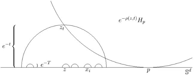
This reflects the fact that this bound does not come from the local dimensions, see Propo-sition 2.8. Suppose δ(Γ) 6 kmax, choose p to be a parabolic fixed point of maximal rank
k(p) = kmax, and let n∈Z+ be a very large integer. Let p6=z0 ∈L(Γ),f be a parabolic
element fixing p, and choose z=fn(z
0)∈L(Γ). Observe thatz6=pand z→pas n→ ∞.
We assumenis large enough to guarantee that the geodesic ray from0toz passes through Hp. Choose T > 0 to be the larger of the two values for which zT lies on the boundary
of Hp (i.e. zT is the ‘exit point’ from Hp). For simplicity, we now restrict our attention
to the 2-dimensional hyperplane H(p, z, zT) containing the pointsp, z, zT and restricted to
Dd+1. Letube the point on the boundary ofHp∩H(p, z, zT) (which is a circle) which is at
hyperbolic distance 1 from zT and lies further away from p thanzT (in Euclidean terms).
Choose t∈(0, T) such that zt∈Hp and such that the geodesic joiningzt and u is normal
Figure 3: ChoosingT and t.
It follows that
ρ(z, t) =dH(zt, u)>dH(zt, zT)−dH(zT, u) =T −t−1.
It follows from (3.1) and the fact thatρ(z, T) =k(z, T) = 0 and k(z, t) =kmaxby
construc-tion, that
µPS(B(z, e−t))
µPS(B(z, e−T)) &
e−t e−T
δ(Γ)
exp(ρ(z, t)(kmax−δ(Γ)))
>
e−t e−T
δ(Γ)
exp((T −t−1)(kmax−δ(Γ)))
&
e−t e−T
kmax .
Finally, basic hyperbolic geometry shows that T −t → ∞ as n → ∞ and therefore dimregµPS > kmax as required. To see why T −t → ∞, switch to the upper half-space
model H2⊆Cand assume that p=∞. Then the boundary ofHp∩H(p, z, zT) is simply a
horizontal Euclidean line and the geodesic ray from 0 (which is represented byi∈H2) to
z is an arc of a circle which meets the boundary at right angles and (linearly) increases in radius with n. Observe that
logIm(zt)
Im(u) =dH(zt, u) =ρ(z, t)6T−t
[image:17.612.178.433.586.689.2]and that Im(u) is fixed but Im(zt) grows without bound inn, see Figure 4.
Figure 4: An explanation of whyT−t→ ∞. For largenthe boundary ofHp appears very
4.2 The lower regularity dimension
The calculation of the lower regularity dimension is similar to the upper regularity dimension and so we only sketch the proof, leaving the details to the reader. The lower bound closely follows the upper bound in the upper regularity case and the upper bound closely follows the lower bound in the upper regularity case. The global measure formula (3.1) is again the key tool and the roles of kmin and kmaxare reversed.
4.2.1 Lower bound: dimregµPS>min{kmin,2δ(Γ)−kmax}
Letz∈L(Γ) andT >t >0. It follows from (3.1) that ifzt andzT lie in the same standard
horoball Hp, then
µPS(B(z, e−t))
µPS(B(z, e−T)) &
e−t e−T
δ(Γ)
exp(ρ(z, t)−ρ(z, T))(k(p)−δ(Γ))
>
e−t e−T
δ(Γ) exp
−(T−t)|k(p)−δ(Γ)| by Lemma 3.1
>
e−t e−T
min{kmin,2δ(Γ)−kmax} .
If zt and zT do not lie in the same standard horoball, then
µPS(B(z, e−t))
µPS(B(z, e−T)) &
e−t e−T
δ(Γ) exp
(ρ(z, t) +ρ(z, T)) min{kmin−δ(Γ), δ(Γ)−kmax}
>
e−t e−T
δ(Γ)
exp(T−t) min{kmin−δ(Γ), δ(Γ)−kmax}
by Lemma 3.1 and since min{kmin−δ(Γ), δ(Γ)−kmax}60
>
e−t e−T
min{kmin,2δ(Γ)−kmax} .
It follows that dimregµPS>min{kmin,2δ(Γ)−kmax}, as required.
4.2.2 Upper bound: dimregµPS6min{kmin,2δ(Γ)−kmax}
Suppose δ(Γ)6kmax, choose pto be a parabolic fixed point of maximal rankk(p) =kmax,
and let ε∈(0,1). By Lemma 3.2 it follows that for T >0 sufficiently large we have
µPS(B(p,1))
µPS(B(p, e−T)) .
1
exp(−δ(Γ)T+ρ(p, T)(kmax−δ(Γ)))
6 1
=
1 e−T
δ(Γ)−(1−ε)(kmax−δ(Γ))
which proves that dimregµPS 62δ(Γ)−kmax+ε(kmax−δ(Γ)) and lettingε→0 provides
the desired upper bound.
Analogous to the upper regularity dimension, showing that dimregµPS 6 kmin is more
subtle since we cannot keep the point z fixed. Suppose δ(Γ)> kmin and choose p to be a
parabolic fixed point of minimal rank k(p) =kmin and let n∈Z+ be a very large integer. Let p 6= z0 ∈L(Γ),f be a parabolic element fixing p, and choose z =fn(z0) ∈L(Γ). As
above, chooseT >0 such thatzT is the ‘exit point’ fromHpand chooset∈(0, T) such that
zt∈Hp andρ(z, t)>T−t−1. It follows from (3.1) and the fact thatρ(z, T) =k(z, T) = 0
and k(z, t) =kmin by construction, that
µPS(B(z, e−t))
µPS(B(z, e−T)) .
e−t e−T
δ(Γ)
exp(ρ(z, t)(kmin−δ(Γ)))
6
e−t e−T
δ(Γ)
exp((T −t−1)(kmin−δ(Γ)))
.
e−t e−T
kmin .
Observe, as before, thatT−t→ ∞asn→ ∞and therefore dimregµPS6kmin as required.
5
The dimensions of
L(Γ)
: proof of Theorem 2.3
5.1 The Assouad dimension
5.1.1 Lower bound: dimAL(Γ)>max{kmax, δ(Γ)}
Since dimAL(Γ)>dimHL(Γ) =δ(Γ) it suffices to prove that dimAL(Γ) >kmax. Letp ∈
L(Γ) be a parabolic fixed point of maximal rank and choose parabolic elementsf1, . . . , fkmax fixingp which are a minimal generating set for a free Abelian groupFmax6Γ lying in the
stabliser of p. Switch to the upper half-space modelHd+1 and assume thatp =∞, which we may do by conjugation which does not alter any dimensions. Therefore fi acts on the
boundary Rdby fi(z) =z+ti for some translation ti∈Rd\ {0}. Observe that theti must
be a linearly independent set or the fi cannot be a minimal generating set for Fmax. Let
z ∈L(Γ)\ {∞} which we know exists since Γ is non-elementary. By Γ-invariance of L(Γ) we have
L(Γ)⊃Γ(z)⊃Fmax(z) =
( z+
kmax X
i=1
niti : (n1, . . . , nkmax)∈Z
kmax )
.
Letα :Rd→Rkmax be an affine map which first sends{t1, . . . , tkmax}to the standard basis in Rkmax and then translates the image of z to the origin. This is a bi-Lipschitz map and so again does not alter any dimensions. It follow that
dimAL(Γ)>dimAα(Fmax(z)) = dimA
Zkmax
To see why dimA Zkmax =kmax consider balls B(0, R) with R tending to ∞ and choose
r = 1/2. Then
Nr
B(0, R)∩Zkmax
= #B(0, R)∩Zkmax &Rkmax &(R/r)kmax
which proves dimA Zkmax>kmax. The other direction is trivial.
5.1.2 Squeezing and counting horoballs
In this section we provide some auxiliary lemmas involving horoballs. Given a horoball Hp
and θ ∈ (0,1], we write θHp ⊆ Hp to denote the squeezed horoball, which still has base
point p but is scaled by a factor of θ. We write |Hp| to denote the Euclidean diameter
of Hp, and thus |θHp| = θ|Hp|. We also write Π : Dd+1 \ {0} →Sd to be the projection defined by choosing Π(z) ∈Sd such that 0, z,Π(z) are collinear with z lying in-between 0
and Π(z). Thus Π(A) is the ‘shadow at infinity’ of a set A⊆Dd+1\ {0}. Note that Π(H
p)
is a ball with Euclidean radius ≈ |Hp|. The following is a well-known result of Stratmann
and Velani [SV, Corollary 3.5].
Lemma 5.1 (Corollary 3.5, [SV]). Let Hp be a standard horoball with base point p ∈ P
and θ∈(0,1] be a ‘squeezing factor’. Then
µPS(Π(θHp))≈θ2δ(Γ)−k(p)|Hp|δ(Γ).
We will also need to be able to count horoballs. This is a standard technique in the study of Kleinian groups, see, for example, [SV]. The following should be interpreted as a partial localisation of [SV, Theorem 1 and 3].
Lemma 5.2. Let z∈L(Γ)and T > t >0. For t sufficiently large we have
X
p∈P∩B(z,e−t):
e−t>|H p|>e−T
|Hp|δ(Γ) . (T −t) µPS(B(z, e−t)).
Proof. It follows from the well-known ‘Dirichlet type Theorem’ for Kleinian groups, see [SV,
Theorem 1], that there is a constant κ >0 depending only on Γ such that for sufficiently larges >0 we have
L(Γ)⊆ [
p∈P:
|Hp|>e−s
Π κ s
e−s |Hp|
Hp
!
with multiplicity.1. In particular, for alls > t >0 with t sufficiently large, the union
[
p∈P∩B(z,e−t):
e−t>|H p|>e−s
Π κ s
e−s |Hp|
Hp
has multiplicity . 1 and is contained in B(z,2e−t). Therefore, applying Lemma 5.1, we have
µPS(B(z,2e−t)) &
X
p∈P∩B(z,e−t):
e−t>|H p|>e−s
µPS Π κ
s e−s
|Hp|
Hp
!!
& X
p∈P∩B(z,e−t):
e−t>|H p|>e−s
κ s
e−s |Hp|
!2δ(Γ)−k(p)
|Hp|δ(Γ)
& e−sδ(Γ) X
p∈P∩B(z,e−t):
e−t>|H p|>e−s
| Hp|
e−s
k(p)/2
> e−sδ(Γ) X
p∈P∩B(z,e−t):
e−t>|Hp|>e−s
1. (5.1)
Therefore
X
p∈P∩B(z,e−t):
e−t>|H p|>e−T
|Hp|δ(Γ) 6
X
m∈Z∩[t,T+1]
X
p∈P∩B(z,e−t):
e−(m−1)>|H
p|>e−m
|Hp|δ(Γ)
. X
m∈Z∩[t,T+1]
X
p∈P∩B(z,e−t):
e−(m−1)>|Hp|>e−m
e−mδ(Γ)
. X
m∈Z∩[t,T+1]
e−mδ(Γ) X
p∈P∩B(z,e−t):
e−t>|Hp|>e−m
1
. X
m∈Z∩[t,T+1]
e−mδ(Γ)emδ(Γ)µPS(B(z,2e−t))
by (5.1)
. (T−t) µPS(B(z, e−t))
since µPS is doubling, which completes the proof.
5.1.3 Upper bound: dimAL(Γ)6max{kmax, δ(Γ)}
Recall that dimAL(Γ) 6 dimregµPS = max{kmax,2δ(Γ)−kmin} and therefore if δ(Γ) 6
(kmin +kmax)/2, then the desired upper bound dimAL(Γ) 6 kmax follows immediately.
From now on we assumeδ(Γ)>(kmin+kmax)/2, although the proof we give actually works
without change in the larger rangeδ(Γ)>kmin. The broad strategy of our argument takes
Let z ∈L(Γ),ε > 0 and T > t > 0 with T −t >max{ε−1,log 10}. Let {x
i}i∈X be a
centrede−T-packing ofB(z, e−t)∩L(Γ) of maximal cardinality, that is,xi∈B(z, e−t)∩L(Γ)
for all i∈X and kxi−xjk>2e−T for alli6=j. Decompose X as the union
X =X0 ∪ X1 ∪
∞
[
n=2
Xn
where
X0=
i∈X : (xi)T ∈Hp with |Hp|>10e−t ,
X1={i∈X\X0 : ρ(xi, T)6ε(T−t)}
and
Xn={i∈X\(X0∪X1) : n−1< ρ(xi, T)6n}.
Note that this is indeed a decomposition because if i /∈ X1, thenρ(xi, T) > ε(T −t) > 1
(by assumption) and so i∈Xnfor somen>2.
We will estimate the cardinalities ofX0,X1 and Xn (n>2) separately, beginning with
X0. An elementary Euclidean volume argument shows that there is at most onep∈P such
that |Hp|>10e−t andHp∩(∪i∈X(xi)T)6=∅. (10 is clearly not the optimal constant here,
but there is no need to optimise it.) Suppose |X0| 6= 0. It follows that we can fix p ∈ P
with |Hp|>10e−t such that (xi)T ∈ Hp for all i∈ X0. Moreover, this forces zt ∈Hp. If
δ(Γ)6k(p), then by (3.1)
(e−t)δ(Γ)exp(−ρ(z, t)(δ(Γ)−k(p))) & µPS(B(z, e−t))
& µPS ∪i∈X0B(xi, e
−T
)
> |X0|min
i∈X0
(e−T)δ(Γ)exp(−ρ(xi, T)(δ(Γ)−k(p)))
since the balls {B(xi, e−T)}i∈X0 are pairwise disjoint. Therefore
|X0| .
e−t e−T
δ(Γ) max
i∈X0
exp((ρ(z, t)−ρ(xi, T)(k(p)−δ(Γ)))
.
e−t e−T
δ(Γ)
exp((T −t)(k(p)−δ(Γ))) by Lemma 3.3
=
e−t e−T
k(p) .
If δ(Γ)> k(p), then we have to work a little harder. In this case, decomposeX0 as
X0 =X00 ∪
∞
[
n=1
X0n
where
and
X0n={i∈X0 : ρ(z, t) +n−1< ρ(xi, T)6ρ(z, t) +n}.
Applying (3.1) we have
(e−t)δ(Γ)exp(−ρ(z, t)(δ(Γ)−k(p))) & µPS(B(z, e−t))
& µPS
∪i∈X0
0B(xi, e
−T)
& |X00|(e−T)δ(Γ)exp(−ρ(z, t)(δ(Γ)−k(p)))
and therefore
|X00|.
e−t e−T
δ(Γ) .
If i∈Xn
0 for somen>1, then the ball B(xi, e−T) is contained in the shadow at infinity of
the squeezed horoball
2e−(ρ(z,t)+n−1)Hp
and therefore
µPS
[
i∈Xn
0
B(xi, e−T)
6 µPS
Π(2e−(ρ(z,t)+n−1)Hp)
. e−(ρ(z,t)+n)(2δ(Γ)−k(p))|Hp|δ(Γ) by Lemma 5.1.
In the other direction, using the fact that {xi}i∈Xn
0 is ane
−T-packing,
µPS
[
i∈Xn
0
B(xi, e−T)
>
X
i∈Xn
0
µPS(B(xi, e−T))
& |X0n|(e−T)δ(Γ)exp(−(ρ(z, t) +n)(δ(Γ)−k(p)))
where the last line comes from (3.1) and the definition of X0n. Therefore
|X0n| . e
−ρ(z,t)|H
p|
e−T
!δ(Γ)
e−nδ(Γ) .
e−t e−T
δ(Γ)
e−nδ(Γ)
where the last inequality uses the estimate
e−ρ(z,t)|Hp| ≈e−t. (5.2)
It is always true that e−ρ(z,t)|Hp|>e−t since zt is on the boundary of e−ρ(z,t)Hp, but the
reverse may not be true in general. However, ife−ρ(z,t)|Hp|>10e−t, say, then the squeezed
Figure 5: Ife−ρ(z,t)|H
p|is much bigger thane−t, then it cannot intersect{(xi)T}i∈X0.
We have
|X0| = |X00|+
∞
X
n=1
|X0n|
.
e−t e−T
δ(Γ) +
∞
X
n=1
e−t e−T
δ(Γ)
e−nδ(Γ)
.
e−t e−T
δ(Γ) .
Therefore, irrespective of the relationship betweenk(p) and δ(Γ), we have the estimate
|X0| .
e−t e−T
max{k(p), δ(Γ)}
6
e−t e−T
max{kmax, δ(Γ)}
. (5.3)
If zt∈Hp with|Hp|610e−t, then
ρ(z, t)6dH(zt, zt−log 10) = log 106T−t
(by assumption) and ifzt∈Hp with|Hp|>10e−tthen eitherX\X0 =∅or there must be
somei∈X\X0 such that xi is not inHp. Then we can apply Lemma 3.3 to obtain
ρ(z, t).T−t. (5.4)
Therefore we may assume the estimate (5.4) when estimating the size of X\X0.
Turning our attention to X1, using (3.1), we have
(e−t)δ(Γ)exp(−ρ(z, t)(δ(Γ)−k(z, t))) & µPS(B(z, e−t))
& µPS ∪i∈X1B(xi, e
−T
)
& X
i∈X1
> |X1|(e−T)δ(Γ)exp(−ε(T −t)(δ(Γ)−kmin))
where the last estimate uses the definition of X1 and our assumption that δ(Γ) > kmin.
Therefore, applying (5.4),
|X1| .
e−t e−T
δ(Γ)
eε(T−t)(δ(Γ)−kmin)e(T−t) max{k(z,t)−δ(Γ),0}
=
e−t e−T
max{k(z,t), δ(Γ)}+ε(δ(Γ)−kmin)
6
e−t e−T
max{kmax, δ(Γ)}+ε(δ(Γ)−kmin)
. (5.5)
Finally, we consider the sets Xn. If i ∈ Xn for n > 2, then ρ(xi, T) > n−1 and
(xi)T ∈ Hp for some p with 10e−t > |Hp| > e−T and, moreover, the ball B(xi, e−T) is
contained in the shadow at infinity of the squeezed horoball
2e−(n−1)Hp.
Since |Hp|<10e−twe also know that p∈B(z,10e−t). For integer k∈[kmin, kmax] let
Xnk = {i∈Xn : k(xi, T) =k}.
For each set Xnk we have
µPS
[
i∈Xk n
B(xi, e−T)
6 µPS
[
p∈P∩B(z,10e−t):
10e−t>|H p|>e−T,
k(p)=k
Π(2e−(n−1)Hp)
6 X
p∈P∩B(z,10e−t):
10e−t>|H p|>e−T,
k(p)=k
µPS(Π(2e−(n−1)Hp))
. e−n(2δ(Γ)−k) X
p∈P∩B(z,10e−t):
10e−t>|H p|>e−T
|Hp|δ(Γ) by Lemma 5.1
. e−n(2δ(Γ)−k)(T−t+ log 10)µPS(B(z, e−t)) by Lemma 5.2
. e−n(2δ(Γ)−k)(T−t)e−tδ(Γ)exp(ρ(z, t)(k(z, t)−δ(Γ))) by (3.1)
by applying (5.4). In the last line we also used the estimate (T −t) 6ε−1n, which holds
providedXn6=∅(which we may assume since we are trying to bound|Xn|from above). In
the other direction, using the fact that {xi}i∈Xk
n is ane
−T-packing, µPS [ i∈Xk n
B(xi, e−T)
>
X
i∈Xk n
µPS(B(xi, e−T))
& |Xnk|(e−T)δ(Γ)exp(−n(δ(Γ)−k)).
Therefore
|Xnk| . ε−1ne−nδ(Γ)e(T−t)δ(Γ)e(T−t) max{k(z,t)−δ(Γ),0} 6 ε−1ne−nδ(Γ)
e−t e−T
max{kmax, δ(Γ)}
and it follows that
|Xn| 6 kmax
X
k=kmin
|Xnk| . ε−1ne−nδ(Γ)
e−t e−T
max{kmax, δ(Γ)}
(5.6)
Finally, combining (5.3), (5.5), and (5.6), we have
|X| = |X0| + |X1| +
∞
X
n=2
|Xn|
.
e−t e−T
max{kmax, δ(Γ)}+ε(δ(Γ)−kmin) +
∞
X
n=2
ε−1ne−nδ(Γ)
e−t e−T
max{kmax, δ(Γ)}
.
e−t e−T
max{kmax, δ(Γ)}+ε(δ(Γ)−kmin)
+ ε−1
e−t e−T
max{kmax, δ(Γ)}
which proves that dimAL(Γ)6max{kmax, δ(Γ)}+ε(δ(Γ)−kmin) and lettingε→0 provides
the desired upper bound.
5.2 The lower dimension of L(Γ)
5.2.1 Upper bound: dimLL(Γ)6min{kmin, δ(Γ)}
The upper bound closely follows the lower bound in the Assouad dimension case, although we rely on a deep result of Bowditch [Bo] which we did not require an analogue of in the Assouad case. Since dimLL(Γ) 6dimHL(Γ) =δ(Γ) it suffices to prove that dimLL(Γ)6
not a conical limit point. Applying the definition of bounded parabolic point to p = ∞, see [Bo, Definition, page 272], one obtains the following lemma. We are grateful to John Parker for bringing this fact to our attention.
Lemma 5.3. There existsλ >0and akmin-dimensional linear subspace V ⊆Rdsuch that L(Γ) ⊆ Vλ ∪ {∞} where Vλ = {x ∈ Rd : infy∈V kx−yk 6 λ} denotes the Euclidean
λ-neighbourhood of V.
Interestingly, this lemma relies on geometric finiteness, see [PS], but our proof of the lower bound in the Assouad dimension case is valid forany non-elementary Kleinian group. Let ∞ 6= z ∈ L(Γ) and consider balls B(z, R) with R tending to ∞ and choose r = 2λ. Then, by Lemma 5.3
Nr(B(z, R)∩L(Γ))6Nr(B(z, R)∩Vλ).(R/r)kmin
which proves dimLL(Γ)6kmin, as required.
5.2.2 Lower bound: dimLL(Γ)>min{kmin, δ(Γ)}
The lower bound is philosophically similar to the upper bound in the Assouad dimen-sion case, although the details turn out to be rather different. Recall that dimLL(Γ) >
dimregµPS = min{kmin,2δ(Γ)−kmax} and therefore if δ(Γ) > (kmax+kmin)/2, then the
desired lower bound dimLL(Γ) >kmin follows immediately and therefore we assume from
now on that δ(Γ)<(kmax+kmin)/26kmax.
Let z ∈ L(Γ), ε ∈ (0,1) and T > t > 1 with T −t > min{ε−1,log 10}. Let
{B(yi, e−T)}i∈Y be a centred e−T-cover of B(z, e−t)∩L(Γ) of minimal cardinality. By
‘centred’ we mean thatyi ∈B(z, e−t)∩L(Γ) for alli∈Y. Decompose Y as the union
Y =Y0 ∪ Y1
where
Y0=
i∈Y : (yi)T ∈Hp with |Hp|>10e−t
and
Y1 =Y \Y0.
Since {B(yi, e−T)}i∈Y is a cover ofB(z, e−t)∩L(Γ) we have
µPS(B(z, e−t)) 6 µPS ∪i∈YB(yi, e−T)
6 µPS ∪i∈Y0B(yi, e
−T
) + µPS ∪i∈Y1B(yi, e
−T
) (5.7)
and therefore at least one of the two terms in (5.7) must be at least µPS(B(z, e−t))/2. We
will consider each of these possibilities separately, beginning with the term involving Y0. In
this case Y0 6=∅ and therefore, as above, we know that we can fixp∈P with|Hp|>10e−t
such that (yi)T ∈Hp for all i ∈Y0 and, moreover, that zt ∈ Hp. If δ(Γ) > k(p), then by
(3.1)
6 2µPS ∪i∈Y0B(yi, e
−T)
. |Y0|max
i∈Y0
(e−T)δ(Γ)exp(−ρ(yi, T)(δ(Γ)−k(p)))
and therefore
|Y0| &
e−t e−T
δ(Γ) min
i∈Y0
exp((ρ(z, t)−ρ(yi, T)(k(p)−δ(Γ)))
&
e−t e−T
δ(Γ)
exp((T −t)(k(p)−δ(Γ))) by Lemma 3.3
=
e−t e−T
k(p)
. (5.8)
Now suppose δ(Γ)< k(p) and write
Y00={i∈Y0 : ρ(yi, T)6ρ(z, t)}.
Ifi∈Y0\Y00thenρ(yi, T)> ρ(z, t) and therefore (yi)T ∈e−ρ(z,t)Hp. The Euclidean distance
from (yi)T toSdise−T ande−ρ(z,t)|Hp| ≈e−t (recall that this is implied byY0\Y00 6=∅, see
(5.2)). Therefore, writing η for the Euclidean radius of e−ρ(z,t)Hp, Pythagoras’ Theorem
guarantees that
kyi−pk6
q
η2−(η−e−T)2 .pηe−T .√e−te−T,
[image:28.612.191.417.444.631.2]see Figure 6.
Figure 6: A right-angled triangle with vertices at (yi)T,pT and the centre ofe−ρ(z,t)Hp.
It follows that B(yi, e−T) is contained in the shadow at infinity of the squeezed horoball
κ0 r
e−T
e−te
−ρ(z,t)H
for someκ0 ≈1. Therefore, by Lemma 5.1, we have
µPS
∪i∈Y
0\Y00B(yi, e
−T)
.
r e−T
e−t
!2δ(Γ)−k(p) µPS
Π
e−ρ(z,t)Hp
≈ e(t−T)(δ(Γ)−k(p)/2)µPS(B(z, e−t))
sincee−ρ(z,t)|H
p| ≈e−t. Sinceδ(Γ)−k(p)/2>0, this proves that forT−tsufficiently large,
balls with centres in Y0\Y00 cannot carry a fixed proportion of theµPS(B(z, e−t)) and so
µPS
∪i∈Y0 0B(yi, e
−T)≈µ
PS ∪i∈Y0B(yi, e
−T)
>µPS(B(z, e−t))/2.
Therefore
(e−t)δ(Γ)exp(ρ(z, t)(k(p)−δ(Γ))) . µPS(B(z, e−t)) by (3.1)
. µPS
∪i∈Y0
0B yi, e
−T
. |Y00|(e−T)δ(Γ)exp(ρ(z, t)(k(p)−δ(Γ)))
by (3.1) and the definition of Y00. This yields
|Y0| > |Y00| &
e−t e−T
δ(Γ)
which, together with (5.8), shows that, irrespective of the relationship between k(p) and δ(Γ), we have the estimate
|Y0| &
e−t e−T
min{k(p), δ(Γ)}
>
e−t e−T
min{kmin, δ(Γ)}
. (5.9)
It remains to consider the case where the second term in (5.7) carries at least half the mass, that is
µPS ∪i∈Y1B(yi, e
−T
)>µPS(B(z, e−t)/2.
Since this guarantees Y1 6=∅, we may assume the estimate (5.4). Write
Y10={i∈Y1 : ρ(yi, T)6ε(T−t)}.
If i∈Y1\Y10 then ρ(yi, T)> ε(T−t) and therefore (yi)T ∈e−ε(T−t)Hp for someHp with
basepoint p ∈ B(z,10e−t) satisfying e−T 6 |Hp| < 10e−t. Since the Euclidean distance
from (yi)T toSd is e−T, we can argue as above (see Figure 6) using Pythagoras’ Theorem to show that
kyi−pk.
q
e−ε(T−t)|H
p|e−T
and therefore B(yi, e−T) is contained in the shadow at infinity of the squeezed horoball
κ00 s
e−ε(T−t)−T |Hp|
for someκ00≈1. Therefore
µPS
∪i∈Y
1\Y10B yi, e
−T
6 X
p∈P∩B(z,10e−t):
10e−t>|H p|>e−T
µPS Π κ00
s
e−ε(T−t)−T |Hp|
Hp
!!
≈ X
p∈P∩B(z,10e−t):
10e−t>|H p|>e−T
s
e−ε(T−t)−T |Hp|
!2δ(Γ)−k(p)
|Hp|δ(Γ)
by Lemma 5.1
6 e−ε(T−t)(δ(Γ)−kmax/2) X
p∈P∩B(z,10e−t):
10e−t>|H p|>e−T
s e−T |Hp|
!2δ(Γ)−k(p)
|Hp|δ(Γ)
6 e−ε(T−t)(δ(Γ)−kmax/2) X
p∈P∩B(z,10e−t):
10e−t>|H p|>e−T
|Hp|δ(Γ)
. e−ε(T−t)(δ(Γ)−kmax/2)(T −t+ log 10)µ
PS(B(z, e−t))
by Lemma 5.2. Since δ(Γ)−kmax/2 >0 this proves that for T −tsufficiently large, balls
with centres in Y1\Y10 cannot carry a fixed proportion ofµPS(B(z, e−t)) and so
µPS
∪i∈Y0 1B(yi, e
−T
)
≈µPS ∪i∈Y1B(yi, e
−T
)>µPS(B(z, e−t)/2.
It then follows from (3.1) that
(e−t)δ(Γ)exp(−ρ(z, t)(δ(Γ)−k(z, t))) . µPS(B(z, e−t))
. µPS
∪i∈Y0 1B(yi, e
−T)
. X
i∈Y0 1
(e−T)δ(Γ)exp(−ρ(yi, T)(δ(Γ)−k(yi, T)))
6 |Y10|(e−T)δ(Γ)exp(ε(T −t)(kmax−δ(Γ)))
where the last estimate uses the definition of Y10 and our assumption that δ(Γ) 6 kmax.
Therefore, applying (5.4),
|Y1| > |Y10| &
e−t e−T
δ(Γ)
eε(T−t)(δ(Γ)−kmax)e(T−t) min{k(z,t)−δ(Γ),0}
=
e−t e−T
>
e−t e−T
min{kmin, δ(Γ)}+ε(δ(Γ)−kmax)
. (5.10)
We have proved that at least one of (5.9) and (5.10) must hold and therefore
|Y| = |Y0|+|Y1| &
e−t e−T
min{kmin, δ(Γ)}+ε(δ(Γ)−kmax)
which proves that dimLL(Γ)>min{kmin, δ(Γ)} −ε(kmax−δ(Γ)) and lettingε→0 provides
the desired lower bound.
6
Local dimensions of
µ
PS: proof of Proposition 2.8
Let z∈L(Γ) andt >0. Then combining (3.1) and the fact thatρ(z, t)6tgives
dimloc(µPS, z) =δ(Γ) + lim sup
t→∞
ρ(z, t)(δ(Γ)−k(z, t))
t 6 δ(Γ) + max{0, δ(Γ)−kmin}
= max{δ(Γ),2δ(Γ)−kmin}
and
dimloc(µPS, z) =δ(Γ) + lim inf
t→∞
ρ(z, t)(δ(Γ)−k(z, t))
t > δ(Γ) + min{0, δ(Γ)−kmax}
= min{δ(Γ),2δ(Γ)−kmax}.
Moreover, the local dimensionδ(Γ) is achieved atµPS-typicalz, see [SV], and ifpa parabolic
fixed point of rank k(p) associated with a standard horoball Hp, then the above estimates
combined with Lemma 3.2 yield
dimloc(µPS, p) = 2δ(Γ)−k(p)
which completes the proof.
Acknowledgements
The author was supported by a Leverhulme Trust Research Fellowship (RF-2016-500). Much of the work was completed while the author was resident at the Institut Mittag-Leffler during the 2017 semester programmeFractal Geometry and Dynamics and is very grateful for the inspiring atmosphere he found there. He is extremely grateful to John Parker for many helpful conversations about Kleinian groups and also thanks Douglas Howroyd for stimulating discussions regarding the regularity dimensions of measures.
References
[AT] J. Angelevska and S. Troscheit. A dichotomy of self-conformal subsets of R with overlaps, preprint, (2016), available at: http://arxiv.org/abs/1602.05821.
[B] A. F. Beardon.The geometry of discrete groups, Graduate Texts in Mathematics, vol. 91, Springer-Verlag, New York, 1983.
[BM] A. F. Beardon and B. Maskit. Limit points of Kleinian groups and finite sided fun-damental polyhedra,Acta Math.,132, (1974), 1–12.
[Be] T. Bedford. Crinkly curves, Markov partitions and box dimensions in self-similar sets,
Ph.D dissertation, University of Warwick, (1984).
[Bi] C. J. Bishop. On a theorem of Beardon and Maskit,Ann. Acad. Sci. Fenn. Math.,21, (1996), 383–388.
[BJ] C. J. Bishop and P. W. Jones. Hausdorff dimension and Kleinian groups,Acta Math.,
179, (1997), 1–39.
[Bo] B. H. Bowditch. Geometrical finiteness for hyperbolic groups, J. Funct. Anal., 113, (1993), 245–317.
[Boy] D. W. Boyd. The residual set dimension of the Apollonian packing, Mathematika,
20, (1973), 170–174.
[CQY] S.Y. Chang, J. Qing and P. C. Yang. On finiteness of Kleinian groups in general dimension, J. Reine Angew. Math.,571, (2004), 1–17.
[F1] K. J. Falconer. Fractal Geometry: Mathematical Foundations and Applications, John Wiley & Sons, Hoboken, NJ, 3rd. ed., 2014.
[F2] K. J. Falconer. Techniques in Fractal Geometry, John Wiley, 1997.
[FM] K. Falk and K. Matsuzaki. The critical exponent, the Hausdorff dimension of the limit set and the convex core entropy of a Kleinian group, Conf. Geom. Dyn., 19, (2015), 159–196.
[Fr] J. M. Fraser. Assouad type dimensions and homogeneity of fractals, Trans. Amer.
Math. Soc.,366, (2014), 6687–6733.
[FH1] J. M. Fraser and D. C. Howroyd. Assouad type dimensions for self-affine sponges,
Ann. Acad. Sci. Fenn. Math.,42, (2017), 149–174.
[FH2] J. M. Fraser and D. C. Howroyd. On the upper regularity dimensions of measures, to appear inIndiana Univ. Math. J., available at: https://arxiv.org/abs/1706.09340. [FHOR] J. M. Fraser, A. M. Henderson, E. J. Olson and J. C. Robinson. On the Assouad
dimension of self-similar sets with overlaps, Adv. Math.,273, (2015), 188–214.
[FY] J. M. Fraser and H. Yu. Arithmetic patches, weak tangents, and dimension, Bull.
Lond. Math. Soc.,50, (2018), 85–95.
[JJKRRS] E. J¨arvenp¨a¨a, M. J¨arvenp¨a¨a, A. K¨aenm¨aki, T. Rajala, S. Rogovin and V. Suo-mala. Packing dimension and Ahlfors regularity of porous sets in metric spaces,Math. Z.,266, (2010), 83–105.
[JV] P. J¨arvi and M. Vuorinen. Uniformly perfect sets and quasiregular mappings, J.
Lon-don Math. Soc.,54, (1996), 515–529.
[KL] A. K¨aenm¨aki and J. Lehrb¨ack. Measures with predetermined regularity and inhomo-geneous self-similar sets, to appear inArk. Mat.,55, (2017), 165–184.
tubu-lar neighborhoods,Indiana Univ. Math. J.,62, (2013), 1861–1889.
[K] M. Kapovich. Kleinian groups in higher dimensions,Geometry and dynamics of groups
and spaces, 487564, Progr. Math., 265, Birkh¨auser, Basel, 2008.
[KV] S.V. Konyagin and A.L. Vol’berg. On measures with the doubling condition, Math.
USSR-Izv.,30, (1988), 629–638.
[L] J. Luukkainen. Assouad dimension: antifractal metrization, porous sets, and homoge-neous measures,J. Korean Math. Soc.,35, (1998), 23–76.
[LS] J. Luukkainen and E. Saksman. Every complete doubling metric space carries a dou-bling measure,Proc. Amer. Math. Soc.,126, (1998), 531–534.
[M] J. M. Mackay. Assouad dimension of self-affine carpets, Conform. Geom. Dyn., 15, (2011), 177–187.
[MT] J. M. Mackay and J. T. Tyson. Conformal dimension. Theory and application, Uni-versity Lecture Series, 54. American Mathematical Society, Providence, RI, 2010. [Ma] B. Maskit. Kleinian groups, Grundlehren der Mathematischen Wissenschaften
[Fun-damental Principles of Mathematical Sciences], vol. 287, Springer-Verlag, Berlin, 1988. [Mat] K. Matsuzaki. The Hausdorff dimension of the limit sets of infinitely generated
Kleinian groups, Math. Proc. Cambridge Philos. Soc.,128, (2000), 123–139.
[MU] D. Mauldin and M. Urba´nski. Dimensions and measures in infinite iterated function systems,Proc. London Math. Soc.,73, (1996), 105–154.
[Mc1] C. McMullen. The Hausdorff dimension of general Sierpi´nski carpets, Nagoya Math. J.,96, (1984), 1–9.
[Mc2] C. McMullen. Hausdorff dimension and conformal dynamics. III. Computation of dimension, Amer. J. Math.,120, (1998), 691–721.
[MPR] G. McShane, J. R. Parker and I. Redfern. Drawing limit sets of Kleinian groups using finite state automata, Exp. Math.,3, (1994), 153–170.
[P] J. R. Parker. Kleinian circle packings,Topology,34, (1995), 489–496.
[PS] J. R. Parker and B. O. Stratmann. Kleinian groups with singly cusped parabolic fixed points, Kodai Math. J.,24, (2001), 169–206.
[Pa] S. J. Patterson. The limit set of a Fuchsian group,Acta Math.,136, (1976), 241–273. [Po] M. Pollicott. Apollonian Circle Packings, online notes available at:
https://homepages.warwick.ac.uk/ masdbl/apollo-29Dec2014.pdf
[R] J. C. Robinson.Dimensions, Embeddings, and Attractors, Cambridge University Press, (2011).
[S] B. O. Stratmann. Weak singularity spectra of the Patterson measure for geometrically finite Kleinian groups with parabolic elements,Michigan Math. J.,46, (1999), 573–587. [SU] B. O. Stratmann and M. Urba´nski. The box-counting dimension for geometrically
finite Kleinian groups, Fund. Math.,149, (1996), 83–93.
[SV] B. O. Stratmann and S. L. Velani. The Patterson measure for geometrically finite groups with parabolic elements, new and old, Proc. Lond. Math. Soc., 71, (1995), 197–220.
[Su] T. Sugawa. Uniform perfectness of the limit sets of Kleinian groups, Trans. Amer.
Math. Soc.,353, (2001), 3603–3615.
[T] P. Tukia. The Hausdorff dimension of the limit set of a geometrically finite Kleinian group,Acta Math.,152, (1984), 127–140.
Jonathan M. Fraser
School of Mathematics and Statistics The University of St Andrews St Andrews, KY16 9SS, Scotland