Using Language Modeling to Select Useful Annotation Data

Using Language Modeling to Select Useful Annotation Data

Dmitriy Dligach

Department of

Computer Science

University of Colorado

at Boulder

Dmitriy.Dligach

@colorado.edu

Martha Palmer

Department of Linguistics

University of Colorado

at Boulder

Martha.Palmer

@colorado.edu

Abstract

An annotation project typically has an abun-dant supply of unlabeled data that can be drawn from some corpus, but because the labeling process is expensive, it is helpful to pre-screen the pool of the candidate instances based on some criterion of future usefulness. In many cases, that criterion is to improve the presence of the rare classes in the data to be annotated. We propose a novel method for solving this problem and show that it com-pares favorably to a random sampling baseline and a clustering algorithm.

1

Introduction

A data set is imbalanced when the distribution of classes in it is dominated by a single class. In Word Sense Disambiguation (WSD), the classes are word senses. The problem of imbalanced data is painfully familiar to WSD researchers: word senses are particularly well known for their skewed distributions that are also highly domain and cor-pus dependent. Most polysemous words have a sense that occurs in a disproportionately high number of cases and another sense that is seen very infrequently. For example, the OntoNotes (Hovy et al., 2006) sense inventory defines two senses for the verb to add. Of all the instances of this verb in the OntoNotes sense-tagged corpus, 93% are the instances of the predominant sense (not the arith-metic sense!). Another fact: there are 4,554 total senses in the OntoNotes sense inventory for 1,713 recently released verbs. Only 3,498 of them are

present in the actual annotated data. More than 1,000 senses (23%) are so rare that they are miss-ing from the corpus altogether. More than a third of the released verbs are missing representative instances of at least one sense. In fact many of the verbs are pseudo-monosemous: even though the sense inventory defines multiple senses, only the most frequent sense is present in the actual anno-tated data. For example, only 1 out of 8 senses of

to rip is present in the data.

The skewed nature of sense distributions is a fact of life. At the same time, a large-scale annota-tion project like OntoNotes, whose goal is the crea-tion of a comprehensive linguistic resource, cannot simply ignore it. That a sense is rare in a corpus does not mean that it is less important to annotate a sufficient number of instances of that sense: in a different domain it can be more common and not having enough annotated instances of that sense could jeopardize the success of an automatic cross-domain WSD system. For example, sense 8 of to rip ("to import an audio file directly from CD") is extremely popular on the web but it does not exist at all in the OntoNotes data. Only the traditional sense of to swap exists in the data but not the com-puter science sense ("to move a piece of program into memory"), while the latter can conceivably be significantly more popular in technical domains.

classifi-er, we conducted 50 supervised learning experi-ments. In each experiment one instance of this verb was selected at random and used for testing while the rest was used for training a maximum entropy model. The resulting confusion matrix shows that the model correctly classified most of the instances of the two predominant senses while misclassify-ing the other classes. The vast majority of the er-rors came from confusing other senses with sense 5 which is the most frequent sense of to call. Clearly, the data imbalance problem has a significant nega-tive effect on performance.

Let us now envision the following realistic sce-nario: An annotation project receives funds to sense-tag a set of verbs in a corpus. It may be the case that some annotated data is already available for these verbs and the goal is to improve sense coverage, or no annotated data is available at all. But it turns out there are only enough funds to an-notate a portion (e.g. half) of the total instances. The question arises how to pre-select the instances from the corpus in a way that would ensure that all the senses are as well represented as possible. Be-cause some senses of these verbs are very rare, the pool of instances pre-selected for the annotation should include as many as possible instances of the rare senses. Random sampling – the simplest ap-proach – will clearly not work: the pre-selected data will contain roughly the same proportion of the rare sense instances as the original set.

If random sampling is not the answer, the data must be selected in some non-uniform way, i.e. using selective sampling. Active learning (e.g. Chen et al., 2006) is one approach to this problem. Some evidence is available (Zhu and Hovy, 2007) that active learning outperforms random sampling in finding the instances of rare senses. However, active learning has several shortcomings: (1) it re-quires some annotated data to start the process; (2) it is problematic when the initial training set only contains the data for a single class (e.g. the pseudo-monosemous verbs); (3) it is not always efficient in practice: In the OntoNotes project, the data is an-notated by two human taggers and the disagree-ments are adjudicated by the third. In classic active learning a single instance is labeled on each itera-tion This means the human taggers would have to wait on each other to tag the instance, on the adju-dicator for the resolution of a possible disagree-ment, and finally on the system which still needs to be-retrained to select the next instance to be

la-beled, a time sink much greater than tagging addi-tional instances; (4) finally, active learning may not be an option if the data selected needs to be manually pre-processed (e.g. sentence segmented, tokenized, and treebanked – as was the case with some of the OntoNotes data). In this setting, on each iteration of the algorithm, the taggers have to also wait for the selected instance to be manually pre-processed before they can label it.

Thus, it would be significantly more convenient if all the data to be annotated could be pre-selected

in advance. In this paper we turn to two unsuper-vised methods which have the potential to achieve that goal. We propose a simple language modeling-based sampling method (abbreviated as LMS) that increases the likelihood of seeing rare senses in the pre-selected data. The basic approach is as follow: using language modeling we can rank the instances of the ambiguous verb according to their probabili-ty of occurrence in the corpus. Because the in-stances of the rare senses are less frequent than the instances of the predominant sense, we can expect that there will be a higher than usual concentration of the rare sense instances among the instances that have low probabilities. The method is completely unsupervised and the only resource that it requires is a Language Modeling toolkit such as SRILM (Stolcke, 2002), which we used in our experiments. We compare this method with a random sampling baseline and semi-supervised clustering, which can serve the same purpose. We show that our method outperforms both of the competing approaches. We review the relevant literature in section 2, explain the details of LMS in section 3, evaluate LMS in section 4, discuss the results in section 5, and de-scribe our plans for future work in section 6.

2

Relevant Work

ones (Weiss, 1995; Japkowicz, 2001). Learning from imbalanced sets can also be problematic if the data is noisy: given a sufficiently high level of background noise, a learner may not distinguish between true exceptions (i.e. rare cases) and noise (Kubat and Matwin, 1997; Weiss, 2004).

In the realm of supervised learning, cost-sensitive learning has been recommended as a so-lution to the problem of learning from imbalanced data (e.g. Weiss, 2004). However, the costs of mis-classifying the senses are highly domain specific and hard to estimate. Several studies recently ap-peared that attempted to apply active learning prin-ciples to rare category detection (Pelleg and Moore, 2004; He and Carbonell, 2007). In addition to the issues with active learning outlined in the introduction, the algorithm described in (He and Carbonell, 2007) requires the knowledge of the priors, which is hard to obtain for word senses.

WSD has a long history of experiments with unsupervised learning (e.g. Schutze, 1998; Puran-dare and Peterson, 2004). McCarthy et al. (2004) propose a method for automatically identifying the predominant sense in a given domain. Erk (2006) describes an application of an outlier detection al-gorithm to the task of identifying the instances of unknown senses. Our task differs from the latter two works in that it is aimed at finding the in-stances of the rare senses.

Finally, the idea of LMS is similar to the tech-niques for sentence selection based on rare n-gram co-occurrences used in machine translation (Eck et al., 2005) and syntactic parsing (Hwa, 2004).

3

Language Modeling for Data Selection

Our method is outlined in Figure 1:

Input

A large corpus that contains Tcandidate instances from which S instances are to be selected for anno-tation

Basic Steps

1. Compute the language model for the corpus 2. Compute the probability distribution over the T candidate instances of the target verb

3. Rank the T candidate instances by their proba-bilities

4. Form a cluster by selecting S instances with the lowest probability

Figure 1. Basic steps of LMS

Let us now clarify a few practical points. Al-though an instance of the target verb can be represented as the entire sentence containing the verb, from the experiments with automatic WSD (e.g. Dligach and Palmer, 2008), it is known that having access to just a few words in the neighbor-hood of the target verb is sufficient in many cases to predict the sense. For the purpose of LMS we represent an instance as the chunk of text centered upon the target verb plus the surrounding words on both sides within a three-word window. Although the size of the window around the target verb is fixed, the actual number of words in each chunk may vary when the target verb is close to the be-ginning or the end of sentence. Therefore, we need some form of length normalization. We normalize the log probability of each chunk by the actual number of words to make sure we do not favor shorter chunks (SRILM operates in log space). The resulting metric is related to perplexity: for a se-quence of words W = w1w2 … wN the perplexity is

N N w w w P W PP

1

2 1 ... ) (

)

( = −

The log of perplexity is

)] ... ( log[ 1 )] (

log[ P w1w2 wN

N W PP =−

Thus, the quantity we use for ranking is nega-tive perplexity.

4

Evaluation

For the evaluation, we selected two-sense verbs from the OntoNotes data that have at least 100 in-stances and where the share of the rare sense is less than 20%. There were 11 such verbs (2,230 in-stances total) with the average share of the rare sense 11%.

rather to group them into a cluster where the rare senses will have a higher concentration than in the original set of the candidate instances. At the same time achieving high recall is important since we want to ensure that most, if not all, of the rare senses that were present among the candidate in-stances are captured in the rare sense cluster.

4.1

The goal of our first set of experiments is to illu-strate the plausibility of LMS. Due to space con-straints, we examine only two verbs: compareand

add. The remaining experiments will focus on a more comprehensive evaluation that will involve all 11 verbs. We computed the normalized log probability for each instance of a verb. We then ordered these candidate instances by their norma-lized log probability and computed the recall of the rare sense at various levels of the size of the rare sense cluster. We express the size of the rare sense cluster as a share of the total number of instances. We depict recall vs. cluster size with a dotted curve. The graphs are in Figures 2 and 3.

Figure 2. Rare sense recall for compare

Figure 3. Rare sense recall for add

The diagonal line on these figures corresponds to the random sampling baseline. A successful

LMS would correspond to the dotted curve lying above the random sampling baseline, which hap-pens to be the case for both of these verbs. For

compare we can capture all of the rare sense in-stances in a cluster containing less than half of the candidate instances. While verbs like compare re-flect the best-case scenario, the technique we pro-posed still works for the other verbs although not always as well. For example, for add we can recall more than 70% of the rare sense instances in a cluster that contains only half of all instances. This is more than 20 percentage points better than the random sampling baseline where the recall of the rare sense instances would be approximately 50%.

4.2

In this experiment we evaluated the performance of LMS for all 11 verbs. For each verb, we ranked the instances by their normalized log probability and placed the bottom half in the rare sense cluster. The results are in Table 2. The second column shows the share of the rare sense instances in the entire corpus for each verb. Thus, it represents the precision that would be obtained by random sam-pling. The recall for random sampling in this set-ting would be 0.5.

Ten verbs outperformed the random sampling baseline both with respect to precision and recall (although recall is much more important for this task) and one verb performed as well. On average these verbs showed a recall figure that was 22 per-centage points better than random sampling. Two of the 11 verbs (compare and point) were able to recall all of the rare sense instances.

Verb Rare Inst Precision Recall account 0.12 0.21 0.93

add 0.07 0.10 0.73

admit 0.18 0.18 0.50 allow 0.06 0.07 0.62 compare 0.08 0.16 1.00 explain 0.10 0.12 0.60 maintain 0.11 0.11 0.53 point 0.15 0.29 1.00 receive 0.07 0.08 0.60 remain 0.15 0.20 0.65 worry 0.15 0.22 0.73 average 0.11 0.16 0.72

4.3

Since LMS is a form of clustering one way to eva-luate its performance is by comparing it with an established clustering algorithm such as K-means (Hastie et al., 2001). There are several issues re-lated to this evaluation. First, K-means produces clusters and which cluster represents which class is a moot question. Since for the purpose of the eval-uation we need to know which cluster is most closely associated with a rare sense, we turn K-means into a semi-supervised algorithm by seeding the clusters. This puts LMS at a slight disadvan-tage since LMS is a completely unsupervised algo-rithm, while the new version of K-means will require an annotated instance of each sense. How-ever, this disadvantage is not very significant: in a real-world application, the examples from a dictio-nary can be used to seed the clusters. For the pur-pose of this experiment, we simulated the examples from a dictionary by simply taking the seeds from the pool of the annotated instances we identified for the evaluation. K-means is known to be highly sensitive to the choice of the initial seeds. Therefore, to make the comparison fair, we perform the clustering ten times and pick the seeds at random for each iteration. The results are aver-aged.

Second, K-means generates clusters of a fixed size while the size of the LMS-produced clusters can be easily varied. This advantage of the LMS method has to be sacrificed to compare its perfor-mance to K-means. We compare LMS to K-means by counting the number of instances that K-means placed in the cluster that represents the rare sense and selecting the same number of instances that have the lowest normalized probability. Thus, we end up with the two methods producing clusters of the same size (with k-means dictating the cluster size).

Third, K-means operates on vectors and there-fore the instances of the target verb need to be represented as vectors. We replicate lexical, syn-tactic, and semantic features from a verb sense dis-ambiguation system that showed state-of-the-art performance on the OntoNotes data (Dligach and Palmer, 2008).

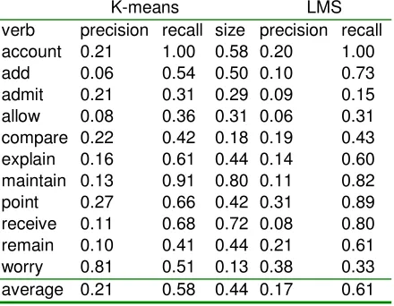
The results of the performance comparison are shown in Table 3. The fourth column shows the relative size of the K-means cluster that was seeded with the rare sense. Therefore it also

de-fines the share of the instances with the lowest normalized log probability that are to be included in the LMS-produced rare sense clusters. On aver-age, LMS showed 3% better recall than K-means clustering.

K-means LMS

verb precision recall size precision recall

account 0.21 1.00 0.58 0.20 1.00

add 0.06 0.54 0.50 0.10 0.73

admit 0.21 0.31 0.29 0.09 0.15

allow 0.08 0.36 0.31 0.06 0.31

compare 0.22 0.42 0.18 0.19 0.43

explain 0.16 0.61 0.44 0.14 0.60

maintain 0.13 0.91 0.80 0.11 0.82

point 0.27 0.66 0.42 0.31 0.89

receive 0.11 0.68 0.72 0.08 0.80

remain 0.10 0.41 0.44 0.21 0.61

worry 0.81 0.51 0.13 0.38 0.33

average 0.21 0.58 0.44 0.17 0.61

Table 3. LMS vs. K-means

5

Discussion and Conclusion

In this paper we proposed a novel method we termed LMS for pre-selecting instances for annota-tion. This method is based on computing the prob-ability distribution over the instances and selecting the ones that have the lowest probability. The ex-pectation is that instances selected in this fashion will capture more of the instances of the rare classes than would have been captured by random sampling. We evaluated LMS by comparing it to random sampling and showed that LMS outper-forms it. We also demonstrated that LMS com-pares favorably to K-means clustering. This is despite the fact that the cluster sizes were dictated by K-means and that K-means had at its disposal much richer linguistic representations and some annotated data.

6

Future Work

First, we would like to investigate the effect of se-lective sampling methods (including LMS) on the performance of WSD models learned from the se-lected data. Next, we plan to apply LMS for Do-main adaptation. Unlike the scenario we dealt with in this paper, the language model would have to be learned from and applied to different corpora: it would be trained on the source corpus and used to compute probabilities for the instances in the target corpus that needs to be adapted. We will also expe-riment with various outlier detection techniques to determine their applicability to data selection. Another promising direction is a simplified active learning approach in which a classifier is trained on the labeled data and applied to unlabeled data; the instances with a low classifier's confidence are selected for annotation (i.e. this is active learning conducted over a single iteration). This approach is more practical than the standard active learning for the reasons mentioned in Section 1 and should be compared to LMS. Finally, we will explore the utility of LMS-selected data as the initial training set for active learning (especially in the cases of the pseudo-monosemous verbs).

Acknowledgments

We gratefully acknowledge the support of the Na-tional Science Foundation Grant NSF-0715078, Consistent Criteria for Word Sense Disambigua-tion, and the GALE program of the Defense Ad-vanced Research Projects Agency, Contract No. HR0011-06-C-0022, a subcontract from the BBN-AGILE Team. Any opinions, findings, and con-clusions or recommendations expressed in this ma-terial are those of the authors and do not necessarily reflect the views of the National Science Foundation.

References

Jinying Chen, Andrew Schein, Lyle Ungar, and Martha Palmer. 2006. An Empirical Study of the Behavior of Active Learning for Word Sense Disambiguation. In Proceedings of the HLT-NAACL.

Dmitriy Dligach and Martha Palmer. 2008. Novel Se-mantic Features for Verb Sense Disambiguation. In Proceedings of ACL-HLT.

Matthias Eck, Stephan Vogel, and Alex Waibel. 2005. Low Cost Portability for Statistical Machine

Transla-tion Based on N-gram Frequency and TF-IDF. Pro-ceedings of IWSLT 2005.

Katrin Erk. Unknown Word Sense Detection as Outlier Detection. 2006. In Proceedings of HLT-NAACL. Trevor Hastie, Robert Tibshirani, and Jerome Friedman.

The Elements of Statistical Learning. Data Mining, Inference, and Prediction. 2001. Springer.

Jingrui He and Jaime Carbonell. 2007. Nearest-Neighbor-Based Active Learning for Rare Category Detection. NIPS.

Hovy, E.H., M. Marcus, M. Palmer, S. Pradhan, L. Ramshaw, and R. Weischedel. 2006. OntoNotes: The 90% Solution. In Proceedings of the HLT-NAACL. Eduard Hovy and Jingbo Zhu. 2007. Active Learning

for Word Sense Disambiguation with Methods for Addressing the Class Imbalance Problem. In Pro-ceedings of EMNLP.

Rebecca Hwa. 2004. Sample Selection for Statistical Parsing. Computational Linguistics. Volume 30. Is-sue 3.

Natalie Japkowicz. 2001. Concept Learning in the Pres-ence of Between-Class and Within-Class Imbalances. Proceedings of the Fourteenth Conference of the Ca-nadian Society for Computational Studies of Intelli-gence, Springer-Verlag.

Miroslav Kubat and Stan Matwin. 1997. Addressing the curse of imbalanced training sets: one-sided selec-tion. In Proceedings of the Fourteenth International Conference on Machine Learning.

Diana McCarthy, Rob Koeling, Julie Weeds, and John Carroll. 2004. Finding Predominant Word Senses in Untagged Text. In Proceedings of 42nd Annual Meeting of Association for Computational Linguis-tics.

Dan Pelleg and Andrew Moore. 2004. Active Learning for Anomaly and Rare-Category Detection. NIPS. Amruta Purandare and Ted Pedersen. Word Sense

Dis-crimination by Clustering Contexts in Vector and Similarity Spaces. 2004. In Proceedings of the Con-ference on CoNLL.

Hinrich Schutze. 1998 Automatic Word Sense Discrim-ination. Computational Linguistics.

Andreas Stolcke. 2002. SRILM - An Extensible Lan-guage Modeling Toolkit. In Proc. Intl. Conf. Spoken Language Processing, Denver, Colorado.

Gary M. Weiss. 1995. Learning with Rare Cases and Small Disjuncts. Proceedings of the Twelfth Interna-tional Conference on Machine Learning, Morgan Kaufmann.