A Multilinear Approach to the Unsupervised Learning of Morphology

A Multilinear Approach to the Unsupervised Learning of Morphology

Anthony Meyer Indiana University [email protected]

Markus Dickinson Indiana University [email protected]

Abstract

We present a novel approach to the un-supervised learning of morphology. In particular, we use a Multiple Cause Mix-ture Model (MCMM), a type of autoen-coder network consisting of two node layers—hidden and surface—and a matrix of weights connecting hidden nodes to sur-face nodes. We show that an MCMM shares crucial graphical properties with autosegmental morphology. We argue on the basis of this graphical similarity that our approach is theoretically sound. Ex-periment results on Hebrew data show that this theoretical soundness bears out in practice.

1 Introduction

It is well-known that Semitic languages pose prob-lems for the unsupervised learning of morphol-ogy (ULM). For example, Hebrew morpholmorphol-ogy exhibits both agglutinative and fusional processes, in addition to non-concatenative root-and-pattern morphology. This diversity in types of morpho-logical processes presents unique challenges not only for unsupervised morphological learning, but for morphological theory in general. Many previ-ous ULM approaches either handle the concatena-tive parts of the morpholgy (e.g., Goldsmith, 2001; Creutz and Lagus, 2007; Moon et al., 2009; Poon et al., 2009) or, less often, the non-concatenative parts (e.g., Botha and Blunsom, 2013; Elghamry, 2005). We present an approach to clustering morphologically related words that addresses both concatenative and non-concatenative morphology via the same learning mechanism, namely the Multiple Cause Mixture Model (MCMM) (Saund, 1993, 1994). This type of learning has direct con-nections to autosegmental theories of morphology

(McCarthy, 1981), and at the same time raises questions about the meaning of morphological units (cf. Aronoff, 1994).

Consider the Hebrew verbszwkr1 _(‘he remem-bers’) and mzkir (‘he reminds’), which share the root z.k.r. In neither form does this root appear as a continuous string. Moreover, each form inter-rupts the root in a different way. Many ULM al-gorithms ignore non-concatenative processes, as-suming word formation to be a linear process, or handle the non-concatenative processes separately from the concatenative ones (see survey in Ham-marstrom and Borin, 2011). By separating the units of morphological structure from the surface string of phonemes (or characters), however, the distinction between non-concatenative and con-catenative morphological processes vanishes.

We apply the Multiple Cause Mixture Model (MCMM) (Saund, 1993, 1994), a type of auto-encoder that serves as a disjunctive clustering al-gorithm, to the problem of morphological learn-ing. An MCMM is composed of a layer of hid-den nodes and a layer of surface nodes. Like other generative models, it assumes that some subset of hidden nodes is responsible for generating each in-stance of observed data. Here, the surface nodes are features that represent the “surface” properties of words, and the hidden nodes represent units of morphological structure.

An MCMM is well-suited to learn non-concatenative morphology for the same reason that the autosegmental formalism is well-suited to representing it on paper (section 2): the layer of morphological structure is separate from the surface layer of features, and there are no de-pendencies between nodes within the same layer. This intra-layer independence allows each hidden node to associate with any subset of features,

con-1_{We follow the transliteration scheme of the Hebrew}

Tree-bank (Sima’an et al., 2001).

tiguous or discontiguous. We present details of the MCMM and its application to morphology in section 3. Our ultimate goal is to find a ULM framework that is theoretically plausible, with the present work being somewhat exploratory.

1.1 Targets of learning

Driven by an MCMM (section 3), our sys-tem clusters words according to similarities in form, thereby finding form-based atomic building blocks; these building blocks, however, are not necessarily morphemes in the conventional sense. A morpheme is traditionally defined as the cou-pling of a form and a meaning, with the meaning often being a set of one or more morphosyntactic features. Our system, by contrast, discovers build-ing blocks that reside on a level between phono-logical form and morphosyntactic meaning, i.e., on themorphomiclevel (Aronoff, 1994).

Stump (2001) captures this distinction in his classification of morphological theories, distin-guishing incremental and realizational theories. Incremental theories view morphosyntactic prop-erties as intrinsic to morphological markers. Accordingly, a word’s morphosyntactic content grows monotonically with the number of mark-ers it acquires. By contrast, in realizational the-ories, certain sets of morphosyntactic properties

license certain morphological markers; thus, the morphosyntactic properties cannot be inherently present in the markers. Stump (2001) presents considerable evidence for realizational morphol-ogy, e.g., the fact that “a given property may be expressed by more than one morphological mark-ing in the same word” (p. 4).

Similarly, Aronoff (1994) observes that the mapping between phonological and morphosyn-tactic units is not always one-to-one. Often, one morphosyntactic unit maps to more than one phonological form, or vice versa. There are even many-to-many mappings. Aronoff cites the En-glish past participle: depending on the verb, the past participle can by realized by the suffixes -ed

or-en, by ablaut, and so on. And yet for any given verb lexeme, thesamemarker is used for the both the perfect tense and the passive voice, despite the lack of a relationship between these disparate syn-tactic categories. Aronoff argues that the complex-ity of these mappings between (morpho-)syntax and phonology necessitates an intermediate level, namely the morphomic level.

MASC FEM

SG mqwmi mqwmi-t PL mqwmi-im mqwmi-wt

(a)mqwmi‘local’

MASC FEM

SG gdwl gdwl-h PL gdwl-im gdwl-wt

(b)gdwl‘big’

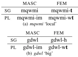
Figure 1: Thetquasi-morpheme

Our system’s clusters correspond roughly to Aronoff’s morphomes. Hence, the system does not require building blocks to have par-ticular meanings. Instead, it looks for pre-morphosyntactic units, i.e., ones assembled from phonemes, but not yet assigned a syntactic or se-mantic meaning. In a larger pipeline, such build-ing blocks could serve as an interface between morphosyntax and phonology. For instance, while our system can find Hebrew’s default masculine suffix-im, it does not specify whether it is in fact masculine in a given word or whether it is fem-inine, as this suffix also occurs in idiosyncratic feminine plurals.

Our system also encounters building blocks like the t in fig. 1, which might be called “quasi-morphemes” since they recur in a wide range of related forms, but fall just short of being entirely systematic.2 _{The t in fig. 1 seems to be} fre-quently associated with the feminine morphosyn-tactic category, as in the feminine nationality suf-fix -it(sinit ‘Chinese (F)’), the suffix -wt for de-riving abstract mass nouns (bhirwt ‘clarity (F)’), as well as in feminine singular and plural present-tense verb endings (e.g., kwtb-t ‘she writes’ and

kwtb-wt‘they (F.PL) write’, respectively).

In fig. 1(a), note that this t is present in both the F.SG and F.PL forms. However, it cannot be assigned a distinct meaning such as “feminine,” since it cannot be separated from thewin theF.PL suffix-wt.3_{Moreover, thistis not always theF.SG} marker; the ending-hin fig. 1(b) is also common. Nevertheless, the frequency with whichtoccurs in feminine words does not seem to be accidental. It seems instead to be some kind of building block, and our system treats it as such.

2_{Though, see Faust (2013) for an analysis positing /-t/ as}

Hebrew’s one (underlying) feminine-gender marker.

3_{If thewin-wtmeant “plural,” we would expect the}

Because our system is not intended to identify morphosyntactic categories, its evaluation poses a challenge, as morphological analyzers tend to pair form with meaning. Nevertheless, we tentatively evaluate our system’s clusters against the mod-ified output of a finite-state morphological ana-lyzer. That is, we map this analyzer’s abstract mor-phosyntactic categories onto categories that, while still essentially morphosyntactic, correspond more closely to distinctions in form (see section 4).

2 Morphology and MCMMs

In this section, we will examine autosegemental (or multi-linear) morphology (McCarthy, 1981), to isolate the property that allows it to handle non-concatenative morphology. We will then show that because an MCMM has this same property, it is an appropriate computational model for learning non-concatenative morphology.

First, we note some previous work connecting autosegmental morphology to computation. For example, Kiraz (1996) provides a framework for autosegmental morphology within two-level mor-phology, using hand-written grammars. By con-trast, Fullwood and O’Donnell (2013) provide a learning algorithm in the spirit of autosegmen-tal morphology. They sample templates, roots, and residues from Pitmor-Yor processes, where a

residue consists of a word’s non-root phonemes, and atemplatespecifies word length and the word-internal positions of root phonemes. Botha and Blunsom (2013) use mildly context-free grammars with crossing branches to generate words with dis-contiguous morphemes. The present work, in con-trast, assumes nothing about structure beforehand. Other works implement certain components of autosegmental theory (e.g., Goldsmith and Xan-thos, 2009) or relegate it to a certain phase in their overall system (e.g., Rodrigues and ´Cavar, 2005). The present work seeks to simulate autosegmental morphology in a more general and holistic way.

2.1 Multilinear morphology

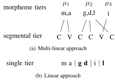
The central aspect of autosegmental theory (Mc-Carthy, 1981) is its multi-linear architecture, i.e., its use of a segmental tier along with many au-tosegmental tiers to account for morphological structure. The segmental tier is a series of place-holders for consonants and vowels, often called theCV skeleton. The other tiers each represent a particular morpheme. Fig. 2(a) shows four tiers.

One is the CV skeleton. The other three, labeled

µ1,µ2, andµ3, are morphemes.4

morpheme tiers

segmental tier _{C V C C V C}

µ1 µ2 µ3

m,a g,d,l i

(a) Multi-linear approach

single tier m a |g d|i|l (b) Linear approach

Figure 2: Multiple tiers vs. a single tier

Notice thatµ2, the consonantal root, is

discon-tinuous; it is interrupted byµ3. If a model has only

one tier, as in fig. 2(b), there would be no way of representing the unity ofµ2, i.e., thatg, d, andl

all belong to the same morpheme. With this multi-tier aspect of autosegmental morphology in mind, we can now state two criteria for a model of non-concatenative morphology:

(1) a. Morphemes are represented as being separate from the segmental tier. b. Each morpheme tier (or node) is

or-thogonal to all other morpheme tiers.

Criterion (1b) implies that the morpheme tiers are unordered. Without sequential dependencies be-tween morpheme tiers, crossing edges such as those in fig. 2(a) are made possible. We should note that autosegmental morphology has other properties to constrain morphological structure, e.g., the well-formedness principle; at present, we are not concerned with capturing all aspects of au-tosegmental morphology, but instead in building a generic system to which one can later add linguis-tically motivated constraints.

2.2 A graph-theoretic interpretation

In graph-theoretic terms, the multi-linear formal-ism of McCarthy (1981) is a type ofmultipartite

graph. This is a graph whose nodes can be parti-tioned intoN sets ofmutually nonadjacentnodes, i.e.,Nsets such that no two nodes within thesame

set are connected by an edge. Fig. 3, for example, shows abipartitegraph, i.e., a graph with two par-titions, in this case the setsMandR. Within each

4_{Although McCarthy uses the termmorphemerather than}

set, all nodes are independent; the only connec-tions are between nodes of different sets.

M

R

Figure 3: Bipartite graph

As it turns out, a bipartite graph suffices to capture the essential properties of McCarthy’s autosegmental framework, for a bipartite graph meets the two criteria stated in (1). We can refor-mulate the morpheme tiers and the segmental tier in fig. 2(a) as the setsM and R, respectively, in fig. 3—disjoint by the definition ofbipartite. This satisfies the first criterion. For the second, each node inM represents a morpheme (or morpheme tier), and, by the definition ofbipartite, the nodes withinM are independent and thus orthogonal.

An MCMM (section 3) is well-suited for the learning of non-concatenative morphology be-cause it is bipartite graph. It has twolayers (equiv-alently, sets) of nodes, a hidden layer and a surface layer—corresponding, respectively, toMandRin fig. 3. There are no intra-layer connections in an MCMM, only connections between layers.

We will henceforth refer to an MCMM’s two partitions of nodes asvectorsof nodes and will use matrix and vector notation to describe the compo-nents of an MCMM: uppercase boldface letters re-fer to matrices, lowercase boldface letters rere-fer to vectors, and italicized lowercase letters refer to the individual elements of vectors/matrices. For ex-ample, mi,k is thekth element in the vector mi,

which is theith_{row in theI×KmatrixM. Thus,}

we will henceforth write theM andRin fig. 3 as

mandr, respectively (ormiandri, whereiis the

index of theith_word).

3 The Multiple Cause Mixture Model

A Multiple Cause Mixture Model (MCMM) (Saund, 1993, 1994) is a graphical model consist-ing of a layer of surface nodes and a hidden layer of causal nodes. The hidden nodes (or units) are connected to surface nodes by weights. Each sur-face node is either ON (active) or OFF (inactive) depending on the hidden-node activities and the weights connecting hidden nodes to surface nodes.

3.1 Architecture

An MCMM can be viewed as a variation of the classical autoencoder network (Dayan and Zemel, 1995), a type of neural network used for unsuper-vised learning. In autoencoders, a hidden layer is forced to learn a compression scheme, i.e., a lower-dimensional encoding, for a dataset.

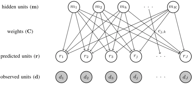
MCMMs are called Multiple Cause Mixture Models because more than one hidden unit can take part in the activation of a surface unit. This is illustrated in figure 4, where the nodesmare the hidden units, and ris the (reconstructed) surface vector. Each arccj,k represents the weight on the

connection betweenmkandrj. The activity ofrj

is determined by a mixing function (section 3.2). The MCMM learns by comparing the recon-structed vectorrito its corresponding original

dat-apoint di. The discrepancy between the two is

quantified by an objective function. If there is a discrepancy, the values of the nodes inmias well

as the weightsCare adjusted in order to reduce the discrepancy as much as possible. See section 3.3 for more on the learning process.

Suppose data pointsdu anddv have some

fea-tures in common. Then, as the MCMM tries to re-construct them inru andrv, respectively,

similar-ities will emerge between their respective hidden-layer vectorsmu andmv. In particular, the

vec-torsmuandmvshould come to share at least one

active node, i.e., at least one k ∈ K such that

mu,k = 1 and mv,k = 1. This can serve as a

basis for clustering; i.e.,mi,k indicates whetherdi

is a member of clusterk. 3.2 Mixing Function

The mapping between the layer of hidden nodesm

and the layer of surface nodesris governed by a

mixing function, which is essentially a voting rule (Saund, 1994); it maps from a set of input “votes” to a single output decision. The output decision is the activity (or inactivity) of a node rij in the

surface layer. Following Saund (1994), we use the Noisy-Or function:

ri,j = 1−

Y

k

(1−mi,kcj,k) (1)

Note that the input to this function includes not only the hidden nodesm, but also theweightscj

on the hidden nodes. That is, the activity of the hidden nodemk is weighted by the valuecjk. A

hidden units (m)

weights (C)

predicted units (r)

observed units (d)

. . .

. . .

. . .

m1 m2 mk mK

r1 r2 r3 rj rJ

d1 d2 d3 dj dJ

cj,k

Figure 4: Architecture of a Multiple Cause Mixture Model (MCMM).

though it is more commonly called an activation functionin autoencoders. The most common ac-tivation function involves a simple weighted sum of the hidden layerm’s activations. The entirely linear weighted sum is then passed to the logistic sigmoid functionσ, which squashes the sum to a number between 0 and 1:

ri,j =σ

X

k

mi,kcj,k

(2)

Notice that both (1) and (2), have the same three primary components: the output (or surface node)

ri,j, the hidden layer of nodesm, and a matrix of

weightsC. Both are possible mixing functions.

3.3 Learning

In both the classical autoencoder and the MCMM, learning occurs as a result of the algorithm’s search for an optimal valuation of key variables (e.g., weights), i.e., a valuation that minimizes the discrepancy between reconstructed and origi-nal data points. The search is conducted via nu-merical optimization; we use the nonlinear conju-gate gradient method. Our objective function is a simple error function, namely the normalized sum of squares error:

E= _I×1_J X

i

X

j

(ri,j−di,j)2 (3)

where I × J is the total number of features in the dataset. The MCMM’s task is to minimize this function by adjusting the values inMandC, whereM is theI ×K matrix that encodes each data point’s cluster-activity vector, and C is the

J ×K matrix that encodes the weights between

miandrifor everyi∈I (see fig. 5).

The MCMM’s learning process is similar to Ex-pectation Maximization (EM) in that at any given time it is holding one set of variables fixed while optimizing the other set. We thus have two func-tions, OPTIMIZE-M and OPTIMIZE-C, which take turns optimizing their respective matrices.

The function OPTIMIZE-M visits each of theI cluster-activity vectorsmiinM, optimizing each

one separately. For eachmi, OPTIMIZE-M enters

an optimization loop over itsK components, ad-justing eachmi,kby a quantity proportional to the

negative gradient ofE atmi,k. This loop repeats

until E ceases to decrease significantly, where-upon OPTIMIZE-M proceeds to the nextmi.

The function OPTIMIZE-C consists of a sin-gle optimization loop over the entire matrix C. Each cj,k is adjusted by a quantity proportional

to the negative gradient of E at cj,k. Unlike

OPTIMIZE-M, which comprises I separate opti-mization loops, OPTIMIZE-C consists of just one, When each of itsJ×Kcomponents has been ad-justed, one round of updates toCis complete. E

is reassessed only between completed rounds of updates. If the change in E remains significant, another round begins.

Both OPTIMIZE-M and OPTIMIZE-C are en-closed within an “alternation loop” that alternates between the two functions, holding Cfixed dur-ing OPTIMIZE-M, and vice versa. This alternation continues untilEcannot be decreased further. At this point, an “outer loop” splits the cluster which contributes the most to the error, adds one to the cluster countK, and restarts the alternation loop. The outer loop repeats until it reaches an overall stopping criterion, e.g.,E= 0.

be-low 0. In other words, it is a task of bound con-strained optimization. Thus, whenever a value in eitherMorCis about to fall below 0, it is set to 0. Likewise, whenever a value is about to exceed 1, it is set to 1 (Ni and Yuan, 1997).

3.4 A Simple MCMM Example

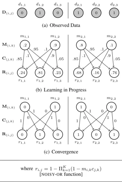
Fig. 5 shows an example of an MCMM for two data points (i.e.,I = 2). The hidden cluster activ-ities M, the weights C, and the mixing function

rconstitute a model that reproduces the observed data points D. The nodes mi,k represent cluster

activities; if m1,2 = 1, for instance, the second

cluster is active for d1 (i.e., d1 is a member of

cluster 2). Note that theJ×Kweight matrixCis the same for all data points, and thekth_{row inC}

can be seen as thekth _{cluster’s “average” vector:}

thejth_{component inc}

kis 1 only if all data points

in clusterkhave 1 at featurej.

D(i,j)

d1,1 d1,2 d1,3 d2,1 d2,2 d2,3

0 1 0 1 0 1

(a) Observed Data

M(i,k)

C(j,k)

R(i,j)

.2 .9 .8 .1

m1,1 m1,2 m2,1 m2,2

.24 .81 .23 .68 .16 .76

r1,1 r1,2 r1,3 r2,1 r2,2 r2,3

.85 .1

.95 .1

.9

.05 .85 .1

.95 .1

.9

.05

(b) Learning in Progress

M(i,k)

C(j,k)

R(i,j)

0 1 1 0

m1,1 m1,2 m2,1 m2,2

0

r1,1 1

r1,2 0

r1,3 1

r2,1 0

r2,2 1

r2,3 1 0

1 0 1

0 1 0

1 0 1

0

(c) Convergence

where ri,j= 1−ΠKk=1(1−mi,kcj,k)

[NOISY-ORfunction]

Figure 5: A simple MCMM example

We can see that while learning is in progress, the cluster activities (mi,k) and the cluster centers

(cj,k) are in flux, as the error rate is being reduced,

but that they converge to values of 0 and 1. At convergence, a reconstruction node (ri,j) is 1 if at

least onemi,kcj,k = 1(and 0 otherwise).

3.5 MCMMs for Morphology

To apply MCMMs to morphological learning, we view the components as follows. For each word

i, the observed (dj) and reconstructed (rj) units

refer to binary surface features extracted from the word (e.g., “the third character iss”). The hidden units (mk) correspond to clusters of words which,

in the ideal case, contain the same morpheme (or morphome). The weights (cj,k) then link specific

morphemes to specific features.

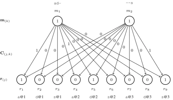
For an example, consider the English wordads. Ideally, there would be two clusters derived from the MCMM algorithm, one for the stem ad and one clustering words with the plural ending -s. Fig. 6 shows a properly learned MCMM, based uponpositionalfeatures: one feature for each let-ter in each position. Note thatadsdoes not have partial membership of thead and-shidden units, but is a full member of both.

4 Experiments 4.1 Gold Standard

Our dataset is the Hebrew word list (6888 unique words) used by Daya et al. (2008) in their study of automatic root identification. This list speci-fies the root for the two-thirds of the words that have roots. Only the roots are specified, how-ever, and not other (non-root) properties. To obtain other morphological properties, we use the MILA Morphological Analysis tool (MILA-MA) (Itai and Wintner, 2008). Because its morphological knowl-edge is manually coded and its output determinis-tic, MILA-MA provides a good approximation to human annotation. The system is designed to an-alyze morphemes, not morphomes, an issue we partially account for in our category mappings and take up further in section 4.4.

As an example of the way we use MILA-MA’s output, consider the wordbycim(‘in trees’), which MILA-MA analyzes as a M%Pl noun bearing the prefixal preposition b- (‘in’). Given this analy-sis, we examine each MCMM-generated cluster that containsbycim. In particular, we want to see if bycimhas been grouped with other words that MILA-MAhas labeled asM%Plor as havingb-.

m(k)

C(j,k)

r(j)

1 1

m1 m2

ad- --s

1

r1 a@1

0

r2 d@1

0

r3 s@1

0

r4 a@2

1

r5 d@2

0

r6 s@2

0

r7 a@3

0

r8 d@3

1

r9 s@3

1 0 0 0 1 0 0 0

0 0

0 0 0 0

0

0 0 1

Figure 6: An MCMM example for the wordads, with nine features (three letters, each at three positions), and two clusters “causing” the word

are irrelevant and are discarded. Each of the 18 re-maining features has at least two values, and some have many more, resulting in a great many feature-value pairs, i.e., categories.

Most part-of-speech (POS) categories are rather abstract; they often cannot be linked to particu-lar elements of form. For example, a noun can be masculine or feminine, can be singular or plural, and can bear one of a variety of derivational af-fixes. But there is no single marker that unifies

allnouns. The situation with verbs is similar: ev-ery Hebrew verb belongs to one of seven classes (binyanim), each of which is characterized by a distinctive vowel pattern.

We thus replace “super-categories” like NOUN andVERBwith finer-grained categories that point to actual distinctions in form. In fact, the only POS categories we keep are those for adverbs, adjec-tives, and numerals (ordinal and cardinal). The rest are replaced by composite (sub-)categories (see below) or discarded entirely, as are negative categories (e.g., construct:false) and un-marked forms (e.g.,M%Sgin nominals).

Sometimes two or more morphosyntactic cate-gories share an element of form; e.g., the future-tense prefix t- can indicate the 2nd person in the MASCgender or, in theFEMgender, either the 2nd or 3rd person:

temwr ‘you (M.SG) will keep’ temwr ‘she will keep’

temwrw ‘you (F.PL) will keep’

Verb inflections are thus mapped to composite cat-egories, e.g., future%(2%M)|(2|3%F), where the symbol | means ‘or’. We also map MILA

-MA’sbinyanandtensefeature-value pairs to stem type, since the shape of a verb’s stem follows from its binyan, and, in some binyanim, past and future tenses have different stems. Both the composite-inflectional andstem type cate-gories represent complex mappings between mor-phosyntax and phonology.

However, since it is not yet entirely clear what would constitute a fair evaluation of the MCMM’s clusters (see section 5), we generally try to retain the traditional morphosyntatctic labels in some form, even if these traditional labels exist only in combination with other labels. Most of our mappings involve fusing “atomic” morphosyntac-tic categories. For example, to capture Hebrew’s fusional plural suffixes for nominals, we combine the atomic categoriesFEMorMASCwithPL; i.e., MASC+PL7→M%PlandFEM+PL7→F%Pl.

Whenever ambiguity is systematic and thus pre-dictable, we choose the most general analysis. For instance, participle analyses are always accom-panied by adjective and noun analyses (cf. En-glish -ing forms). Since a participle is always both a noun and an adjective, we keep the par-ticiple analysis and discard the other two. Finally, we userootless:Nominal to capture ortho-graphic regularities in loan words. In sum, we employ reasonably motivated and informative cat-egories, but the choice of mappings is nontrivial and worthy of investigation in its own right.

4.2 Thresholds and Features

de-creasing significantly, it adds a cluster. It is sup-posed to continue to add clusters until it converges, i.e., until the error is (close to) 0, but so far our MCMM has never converged. As the number of clusters increases, the MCMM becomes increas-ingly encumbered by the sheer number of compu-tations it must perform. We thus stop it when the number of clustersK reaches a pre-set limit: for this paper, the limit wasK = 100. Such a cut-off leaves most of the cluster activities inMbetween 0and1. We set a threshold for cluster membership at0.5: ifmi,kcj,k ≥0.5for at least one indexjin

J, thendiis a member of thekthcluster.

Ifmi,kcj,k ≤0.5for alljinJ, we say that the

kth_{cluster isinactivein thei}th_{word. If a cluster is}

inactive foreveryword, we say that it is currently only apotentialcluster rather than anactualone.

Each word is encoded as a vector of features. This vector is the same length for all words. For any given word, certain features will be ON (with values = 1), and the rest—a much greater portion—will beOFF(with values=0). Each fea-ture is a statement about a word’s form, e.g., “the first letter isb” or “ioccurs beforet”. In our fea-tures, we attempt to capture some of the informa-tion implicit in a word’s visual representainforma-tion.

A positional featureindicates the presence of a particular character at a certain position, e.g., m@[0], for ‘m at the first position’ orl@[-2] for ‘l at the second-to-last position’. Each data pointdi contains positional features

correspond-ing to the firstsand the finalspositions in wordi, wheresis a system parameter (section 4.4). With 22letters in the Hebrew alphabet, this amounts to 22×s×2positional features.

A precedence featureindicates, for two char-actersaandb, whetheraprecedesbwithin a cer-tain distance (or number of characters). This dis-tance is the system parameterδ. We defineδas the difference between the indices of the charactersa

andb. For example, ifδ= 1, then charactersaand

bare adjacent. The number of precedence features is the length of the alphabet squared (222 _{= 484).}

4.3 Evaluation Metrics

We evaluate our clustering results according to three metrics. Let U denote the set of M re-turned clusters andV the set ofN gold-standard categories. The idea behindpurity is to compute the proportion of examples assigned to the correct cluster, using the most frequent category within

a given cluster as gold. Standard purity assumes each example belongs to only one gold category. For a dataset like ours consisting of multi-category examples, this can yield purities greater than 1. We thus modify the calculations slightly to com-puteaverage cluster-wise purity, as in (4), where we divide by M. While this equation yields pu-rities within[0,1], even when clusters overlap, it retains the metric’s bias toward small clusters.

pur_avg(U, V) = _M1 X

m∈M

maxn|um∩vn|

M (4)

Given this bias, we incorporate other metrics: BCubed precision and BCubed recall (Bagga and Baldwin, 1998) compare the cluster mappings ofx with those ofy, for every pair of data points

xandy. These metrics are well-suited to cases of overlapping clusters (Artiles and Verdejo, 2009). Suppose x and y share m clusters and n cate-gories. BCubed precision measures the extent to whichm ≤ n. It is 1 as long there are not more clusters than gold-standard categories. BCubed Recall measures the extent to whichm ≥ n. See Artiles and Verdejo (2009) for calculation details. 4.4 Results

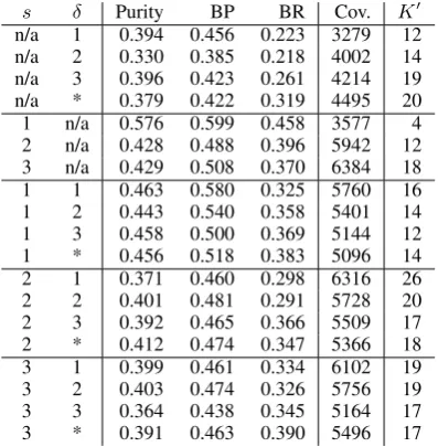
With a cut-off point atK = 100clusters, we ran the MCMM at different valuations ofsandδ. The results are given in table 1, where “δ = ∗” means thatδ is the entire length of the word in question, and “n/a” means that the feature type in question was left out; e.g., in the s column, “n/a” means that no positional features were used. Depending upon the threshold (section 4.2), a cluster may be empty: K0 _{is the number ofactual clusters (see}

section 4.2).Cov(erage), on the other hand, is the number of words that belong to least one cluster. The valuations s = 1 and δ = 1 or 2 seem to produce the best overall results.5

Some of the clusters appear to be capturing key properties of Hebrew morphology, as evidenced by the MILA-MA categories. For example, in one cluster, 677 out of 942 words turn to be of the composite MILA-MA category M%Pl, a pu-rity of 0.72.6 _{In another cluster, this one} contain-ing 584 words, 483 are of theMILA-MAcategory

5_{Whiles = 1indicates an preference for learning short}

prefixes and suffixes, it is important to note that more than one-letter affixes may be learned through the use of the prece-dence features, which can occur anywhere in a word.

6_{Recall that M%Pl is merger of the originally separate}

preposition:l(the prefixal prepositionl-), a purity of 0.83.

Thus, in many cases, the evaluation recognizes the efficacy of the method and helps sort the dif-ferent parameters. However, it has distinct lim-itations. Our gold standard categories are modi-fied categories fromMILA-MA, which are not en-tirely form-based. For example, in one 1016-word cluster, the three most common gold-standard cat-egories areF%Pl(441 words),F%Sg(333 words), andpos:adjective(282 words). Taking the most frequent category as the correct label, the pu-rity of this cluster is 441

1016 = 0.434. However, a

simple examination of this cluster’s words reveals it to be more coherent than this suggests. Of the 1016 words, 92% end int; in 96%,tis one of the final two characters; and in 98%, one of the final three. Whentis not word-final, it is generally fol-lowed by a morpheme and thus is stem-final. In-deed, this cluster seems to have captured almost exactly the “quasi-morpheme”tdiscussed in sec-tion 1. Thus, an evaluasec-tion with more form-based categories might measure this cluster’s purity to be around 98%—a point for future work.

None of the experiments reported here produced

actual (section 4.2) clusters representing conso-nantal roots. However, past experiments did pro-duce some consonantal-root clusters. In these clusters, the roots were often discontinuous, e.g.,

z.k.r in the wordslizkwr, lhzkir, andzikrwn. It is not yet clear to us why these past experiments pro-duced actual root clusters and the present ones did not, but, in any case, we expect to see more root clusters asK(and especiallyK0_{) increases.}

s δ Purity BP BR Cov. K0

n/a 1 0.394 0.456 0.223 3279 12 n/a 2 0.330 0.385 0.218 4002 14 n/a 3 0.396 0.423 0.261 4214 19 n/a * 0.379 0.422 0.319 4495 20 1 n/a 0.576 0.599 0.458 3577 4 2 n/a 0.428 0.488 0.396 5942 12 3 n/a 0.429 0.508 0.370 6384 18 1 1 0.463 0.580 0.325 5760 16 1 2 0.443 0.540 0.358 5401 14 1 3 0.458 0.500 0.369 5144 12 1 * 0.456 0.518 0.383 5096 14 2 1 0.371 0.460 0.298 6316 26 2 2 0.401 0.481 0.291 5728 20 2 3 0.392 0.465 0.366 5509 17 2 * 0.412 0.474 0.347 5366 18 3 1 0.399 0.461 0.334 6102 19 3 2 0.403 0.474 0.326 5756 19 3 3 0.364 0.438 0.345 5164 17 3 * 0.391 0.463 0.390 5496 17

Table 1: Results atK = 100

5 Summary and Outlook

We have presented a model for the unsupervised learning of morphology, the Multiple Cause Mix-ture Model, which relies on hidden units to gener-ate surface forms and maps to autosegmental mod-els of morphology. Our experiments on Hebrew, using different types of features, have demon-strated the potential utility of this method for dis-covering morphological patterns.

So far, we have been stopping the MCMM at a set number (K) of clusters because computa-tional complexity increases withK: the complex-ity is proportional to I ×J ×K, withI ×J al-ready large. But if the model is to find consonan-tal roots along with affixes,K is going to have to be much larger. We can attack this problem by taking advantage of the nature of bipartite graphs (section 2): with intra-layer independence, every

ri,j in the vector ri—and thus each element in

the entire matrixR—can be computedin paral-lel. We are currently parallelizing key portions of our code, rewriting costly loops as kernels to be processed on the GPU.

In a different vein, we intend to adopt a better method of evaluating the MCMM’s clusters, one more appropriate for themorphome-like nature of the clusters. Such a method will require gold-standard categories that are morphomic rather than morphosyntactic, and we anticipate this to be a nontrivial undertaking. From the theoretical side, an exact inventory of (Hebrew) morphomes has not been specified in any work we know of, and annotation criteria thus need to be established. From the practical side, MILA-MA provides nei-ther segmentation nor derivational morphology for anything other than verbs, and so much of the an-notation will have to built from scratch.

Finally, our data for this work consisted of Modern Hebrew words that originally appeared in print. They are spelled according to the or-thographic conventions of Modern Hebrew, i.e., without representing many vowels. As vowel ab-sences may obscure patterns, we intend to try out the MCMM on phonetically transcribed Hebrew.

References

Mark Aronoff. 1994. Morphology by Itself: Stems and

Inflectional Classes, volume 22 ofLinguistic Inquiry

Monograph. MIT Press, Cambridge, MA.

cluster-ing evaluation metrics based on formal constraints.

Information Retrieval12(4):353–371.

Amit Bagga and Breck Baldwin. 1998. Entity-based cross-document coreferencing using the vec-tor space model. InProceedings of the 17th interna-tional conference on Computainterna-tional linguistics:

Vol-ume 1. Association for Computational Linguistics,

pages 79–85.

Jan A. Botha and Phil Blunsom. 2013. Adaptor gram-mars for learning non-concatenative morphology. In

Proceedings of the 2013 Conference on Empirical Methods in Natural Language Processing (EMNLP-13). Seattle, pages 345–356.

Mathias Creutz and Krista Lagus. 2007. Unsupervised models for morpheme segmentation and morphol-ogy learning. ACM Transactions on Speech and

Language Processing4(1):3.

Ezra Daya, Dan Roth, and Shuly Wintner. 2008. Identi-fying semitic roots: Machine learning with linguistic constraints. Computational Linguistics34(3):429– 448.

Peter Dayan and Richard S Zemel. 1995. Competi-tion and multiple cause models. Neural Computa-tion7:565–579.

Khaled Elghamry. 2005. A constraint-based algorithm for the identification of arabic roots. In Proceed-ings of the Midwest Computational Linguistics

Col-loquium. Indiana University.

Noam Faust. 2013. Decomposing the feminine suf-fixes of modern hebrew: a morpho-syntactic anal-ysis. Morphology23(4):409–440.

Michelle Fullwood and Tim O’Donnell. 2013. Learn-ing non-concatenative morphology. InProceedings of the Fourth Annual Workshop on Cognitive

Mod-eling and Computational Linguistics (CMCL). Sofia,

Bulgaria, pages 21–27.

John Goldsmith. 2001. Unsupervised learning of the morphology of a natural language. Computational

Linguistics27:153–198.

John Goldsmith and Aris Xanthos. 2009. Learning phonological categories. Language85(1):4–38. Harald Hammarstrom and Lars Borin. 2011.

Unsuper-vised learning of morphology. Computational

Lin-guistics37(2):309 – 350.

Alon Itai and Shuly Wintner. 2008. Language resources for Hebrew. Language Resources and Evaluation

42(1):75–98.

George Anton Kiraz. 1996. Computing prosodic mor-phology. In Proceedings of the 16th International Conference on Computational Linguistics (COLING

1996). Copenhagen, pages 664–669.

Andreas Kl¨ockner, Nicolas Pinto, Yunsup Lee, B. Catanzaro, Paul Ivanov, and Ahmed Fasih. 2012. PyCUDA and PyOpenCL: A Scripting-Based Ap-proach to GPU Run-Time Code Generation.Parallel

Computing38(3):157–174.

John J McCarthy. 1981. A prosodic theory of noncon-catenative morphology. Linguistic inquiry12:373– 418.

Taesun Moon, Katrin Erk, and Jason Baldridge. 2009. Unsupervised morphological segmentation and clus-tering with document boundaries. InProceedings of the 2009 Conference on Empirical Methods in

Natu-ral Language Processing: Volume 2. Association for

Computational Linguistics, pages 668–677.

Q Ni and Y Yuan. 1997. A subspace limited mem-ory quasi-newton algorithm for large-scale nonlin-ear bound constrained optimization.Mathematics of Computation of the American Mathematical Society

66(220):1509–1520.

Hoifung Poon, Colin Cherry, and Kristina Toutanova. 2009. Unsupervised morphological segmentation with log-linear models. InIn ACL. Ariya Rastrow,

Abhinav Sethy, and Bhuvana Ramabhadran.

Paul Rodrigues and Damir ´Cavar. 2005. Learn-ing arabic morphology usLearn-ing information theory.

In Proceedings from the Annual Meeting of the

Chicago Linguistic Society. Chicago Linguistic

So-ciety, pages 49–58.

Eric Saund. 1993. Unsupervised learning of mixtures of multiple causes in binary data. InNIPS. pages 27–34.

Eric Saund. 1994. A multiple cause mixture model for unsupervised learning. Neural Computation

7(1):51–71.

Khalil Sima’an, Alon Itai, Yoad Winter, Alon Altman, and N. Nativ. 2001. Building a tree-bank of Modern Hebrew text. Traitment Automatique des Langues

42(2).

Gregory T Stump. 2001. Inflectional morphology: A

theory of paradigm structure, volume 93.