Department of Computing
Distributed Abductive Reasoning: Theory,
Implementation and Application
Jiefei Ma
Submitted in part fulfilment of the requirements for the degree of Doctor of Philosophy in Computing of Imperial College London and
I, Jiefei Ma, declare that this thesis is my own work and has not been submitted in any form for another degree or diploma at any university or other institute of tertiary education. Information derived from the published and unpublished work of others has been acknowledged in the text and a list of references is given in the bibliography.
Abductive reasoning is a powerful logic inference mechanism that allows assumptions to be made during answer computation for a query, and thus is suitable for reasoning over incomplete knowledge. Multi-agent hypothetical reasoning is the application of abduction in a distributed setting, where each computational agent has its local knowledge representing partial world and the union of all agents’ knowledge is still incomplete. It is different from simple distributed query processing because the assumptions made by the agents must also be consistent with global constraints.
Multi-agent hypothetical reasoning has many potential applications, such as collaborative plan-ning and scheduling, distributed diagnosis and cognitive perception. Many of these applications require the representation of arithmetic constraints in their problem specifications as well as constraint satisfaction support during the computation. In addition, some applications may have confidentiality concerns as restrictions on the information that can be exchanged between the agents during their collaboration. Although a limited number of distributed abductive sys-tems have been developed, none of them is generic enough to support the above requirements.
In this thesis we develop, in the spirit of Logic Programming, a generic and extensible dis-tributed abductive system that has the potential to target a wide range of disdis-tributed problem solving applications. The underlying distributed inference algorithm incorporates constraint satisfaction and allows non-ground conditional answers to be computed. Its soundness and completeness have been proved. The algorithm is customisable in that different inference and coordination strategies (such as goal selection and agent selection strategies) can be adopted while maintaining correctness. A customisation that supports confidentiality during problem solving has been developed, and is used in application domains such as distributed security policy analysis. Finally, for evaluation purposes, a flexible experimental environment has been built for automatically generating different classes of distributed abductive constraint logic pro-grams. This environment has been used to conduct empirical investigation of the performance of the customised system.
I would like to express my deepest gratitude to my co-supervisors Dr. Alessandra Russo and Dr. Krysia Broda. This thesis would not have been possible without their advice, encouragement, support and guidance. I am also very thankful to my second supervisor Dr. Emil Lupu, whose constructive criticism and invaluable insights were very inspiring and motivational. I would like to express my wholehearted gratitude to all of my supervisors and Professor Morris Sloman for organising the financial support required for me to pursue my PhD studies.
I would also like to thank my PhD examiners Professor Marek Sergot (internal) and Professor Antonis Kakas (external) from University of Cyprus for their very constructive criticism and detailed comments that help improve this thesis.
I am grateful to the academic staff and researchers in the Department of Computing for their guidance and technical advice, in particular Professor Keith Clark, Dr. Francesca Toni, Profes-sor Murray Shanahan and ProfesProfes-sor Morris Sloman. I am also grateful to ProfesProfes-sor Ken Satoh and Professor Hiroshi Hosobe of the National Institute of Informatics (Japan), and Dr. Jorge Lobo and Dr. Seraphin Calo of the IBM T. J. Watson Research Center (USA) for their helpful advice and discussions related to my PhD studies.
Many thanks to my fellow students and friends who have been part of Office 502 or in the Policy research group, namely Dalal Alrajeh, Rudi Ball, Themis Bourdenas, Domenico Corapi, Robert Craven, Luke Dickens, Changyu Dong, Anandha Gopalan, Sye-loong Keoh, Jim Kuo, Srdjan Marinovic, Encrico Scalavino, Alberto Schaeffer-Filho, Vrizlynn Thing and Ryan Wishart, for their friendship and support.
My most profound gratitude goes to my parents, MA Xincai and SHI Baolan, to whom this thesis is dedicated. They provided me with constant care, encouragement and inspiration to never give up.
The work presented in this thesis was partly funded by: the Imperial College London Deputy Rector’s Award 2007–2010; the International Technology Alliance sponsored by the U.S. Army Research Laboratory and the U.K. Ministry of Defence under Agreement Number W911NF-06-3-0001.
Acknowledgements v 1 Introduction 1 1.1 Motivations . . . 1 1.2 Summary of Contributions . . . 4 1.3 Thesis Overview. . . 7 2 Background 9 2.1 First-Order Logic Language and Semantics . . . 9
2.1.1 Herbrand Models . . . 12
2.2 Logic Programming . . . 13
2.2.1 Syntax . . . 13
2.2.2 Semantics . . . 14
2.2.3 Operational Semantics of Logic Programs . . . 22
2.2.4 Constraint Logic Programming . . . 23
2.3 Abductive Logic Programming. . . 24
2.3.1 Abductive Reasoning . . . 24
2.3.2 Abductive Logic Programs . . . 25
2.3.3 Semantics for Abduction . . . 26
2.3.4 Abductive Proof Procedures . . . 28
3 Early Work – Distributed Abductive REasoning (DARE) 36 3.1 Introduction . . . 36
3.2 The Centralised Meeting Scheduling Example . . . 38
3.3 DARE Framework and Algorithm . . . 41
3.3.1 Overview . . . 42
3.3.2 Distributed Algorithm . . . 44
3.3.3 Distributed Meeting Scheduling Example . . . 52
3.4 DARE Implementation . . . 57
3.4.1 Impact of Openness. . . 58
3.4.2 Termination . . . 59
3.5 Limitations of DARE . . . 61
3.6 Conclusion . . . 63
4 Distributed Abductive REasoning with Constraints (DAREC) 65 4.1 Introduction . . . 65
4.2 Distributed Framework for Fixed Agent Systems . . . 69
4.3 Distributed Algorithm . . . 73
4.3.2 Notations of State + Local Abductive Derivation . . . 75
4.3.3 Local Abductive Inference Rules. . . 78
4.3.4 Coordination . . . 88
4.3.5 Example Trace . . . 96
4.4 Soundness and Completeness. . . 98
4.4.1 Soundness . . . 100
4.4.2 Completeness . . . 106
4.5 Discussions . . . 114
4.5.1 Usage of Agent Advertisements . . . 114
4.5.2 Extension for Open Agent Systems . . . 115
4.6 Conclusion . . . 116
5 Multi-agent Hypothetical Reasoning with Confidentiality (DAREC2) 119 5.1 Introduction . . . 119
5.2 Distributed Framework with Confidentiality . . . 124
5.3 Distributed Abduction with Confidentiality. . . 128
5.3.1 Customisation of the Local Inference Rules . . . 129
5.3.2 Customisation of the Coordination . . . 135
5.3.3 Sample Execution Trace of DAREC2 . . . 137
5.4 Discussions . . . 139
5.4.1 Confidential Reasoning by DAREC2 . . . 139
5.4.3 Soundness and Completeness of DAREC2 . . . 141
5.5 Implementation of DAREC2 . . . 141
5.5.1 Agent Knowledge Specifications . . . 143
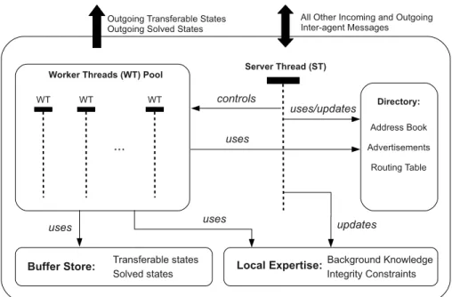
5.5.2 Overview of the Agent Architecture . . . 144
5.5.3 Agent Communications . . . 147
5.5.4 Protocols for Agent Joining, Leaving and Knowledge Update . . . 148
5.5.5 Executions of the Server Thread and the Worker Threads . . . 152
5.6 Related Work . . . 160
5.6.1 Centralised Abductive Systems . . . 160
5.6.2 Distributed Abductive Systems . . . 161
5.6.3 Speculative Multi-agent Reasoning Systems . . . 163
5.7 Conclusion . . . 164
6 Experiments and Benchmarking 166 6.1 A Random Generator for Distributed Abductive Constraint Logic Programs (GenDACLP) . . . 167
6.1.1 The Input and Output of the GenDACLP . . . 168
6.1.2 Implementation of GenDACLP . . . 172
6.2 Experiments and Discussions. . . 177
6.2.1 Environmental Setup . . . 177
6.2.2 Experiments . . . 178
7 Distributed Policy Analysis 188
7.1 Introduction . . . 188
7.2 A Formal Framework for Centralised Policy Analysis . . . 191
7.2.1 Operational Model . . . 191
7.2.2 System Specification . . . 193
7.2.3 Example Policy Analysis Tasks . . . 198
7.3 Extended Framework for Distributed Policy Analysis . . . 201
7.3.1 Extending the Operational Model and the Language . . . 201
7.3.2 Distributed Policy Analysis . . . 206
7.4 Discussions . . . 214
7.5 Conclusion . . . 216
8 Conclusion and Future Work 218 A Example Source Code 221 A.1 The Inequality Solver . . . 221
Bibliography 225
2.1 Kleene’s 3-Valued Logic . . . 20
2.2 Kleene’s Equivalence ↔k vs. Strong Equivalence ↔s . . . 20
5.1 DAREC2 Inter-agent Communication Message Types . . . 154
5.2 DAREC2 Inter-thread (between ST and WTs) Communication Message Types . 157
6.1 List of Input Parameters for GenDACLP . . . 168
6.2 Experiment A (Collected Data(: all thesetswithin atestused the same configuration except the randomly number generator seed for the GenDACLP . . . 181
6.3 Experiment B (Collected Data(: all thesets within atestused the same configuration except the randomly number generator seed for the GenDACLP . . . 184
7.1 Predicates inL =LΠ I ∪ LΠO∪ LΠS ∪ L Gd E ∪ L D S . . . 194 xiii
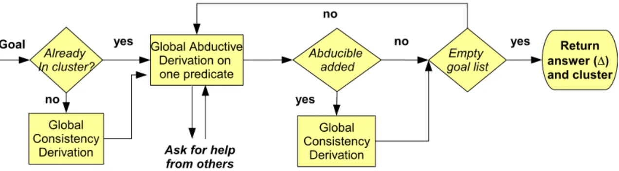
3.1 Global Abductive Derivation . . . 46
3.2 Global Consistency Derivation . . . 46
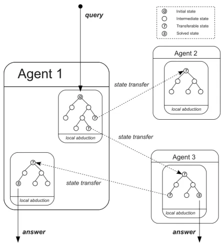
4.1 Distributed Abduction . . . 74
4.2 Pseudo-code of DAREC Agent Execution. . . 93
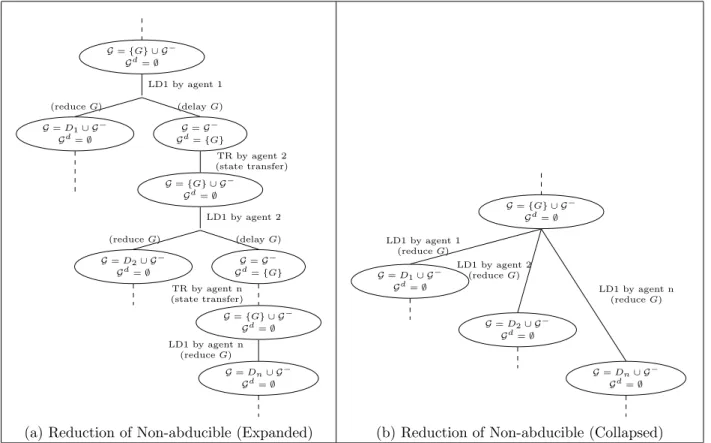
4.3 DAREC Derivation Tree with Pseudo-ASystem Execution Strategy (Reduction of Non-abducible Goal) . . . 109
4.4 DAREC Derivation Tree with Pseudo-ASystem Execution Strategy (Reduction of Abducible or Non-abducible Constraint) . . . 110
4.5 Transformation of Derivations involving LD2 and TR . . . 112
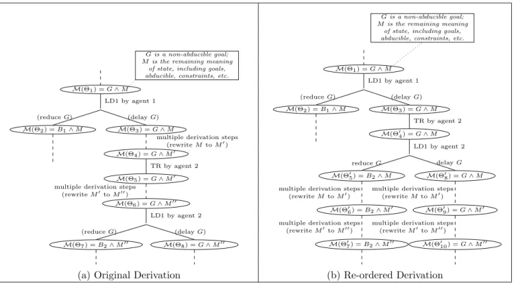
4.6 Transformation of Derivations involving LD1 and TR . . . 113
5.1 DAREC2 Agent Internal Architecture. . . 145
5.2 Changing of Leader . . . 149
5.3 New Agent Joining the System . . . 150
5.4 Existing Agent Leaving the System . . . 151
5.5 Update of Agent Knowledge . . . 152
contain the query ID, and the ST of each agent can use it to identify its corresponding
WT. . . 156
5.7 Usage of the State Buffer by a WT . . . 159
5.8 State Chart Diagram of WT’s Life Cycle . . . 160
5.9 Execution Flow Charts of WT . . . 165
6.1 Example Configuration File for GenDACLP (sample.config) . . . 171
6.2 Example Output File for GenDACLP (total.pl) . . . 172
6.3 Key Steps of the GenDACLP . . . 173
6.4 Pseudo-code for Filling Arguments . . . 174
6.5 Experiment A: Average Centralised/Distributed Computation Time vs. Number of Agents (Size of the Overall Logic Program) . . . 180
6.6 Experiment A: Communication Cost vs. Messages Exchanged . . . 182
6.7 Experiment A: Average Distributed Computation Time vs. Messages Exchanged . . . 182
6.8 Experiment B: Average Centalised/Distributed Computation Time vs. Number of Agents . . . 183
6.9 Experiment B: Average Distributed Computation Time vs. Number of Agents . . . . 185
6.10 Experiment B: Communication Cost vs. Messages Exchanged . . . 185
6.11 Experiment B: Average Distributed Computation Time vs. Messages Exchanged . . . 186
7.1 A Policy Enforcement Point . . . 189
7.2 Operational Model with Centralised PEP/PDP . . . 192
7.3 Coalition Network with Multiple PEPs/PDPs . . . 201
Introduction
1.1
Motivations
Abductive reasoning is a powerful mechanism for reasoning with incomplete knowledge. It can be viewed as a process of finding explanation for an observation, or as a process of generating conditional proofs for a conclusion. The conditions of the proof are abduced assumptions that, together with a given knowledge-base, imply the conclusion of the proof. Abduced assumptions can be viewed, within the context of a knowledge-base, as an explanation of the conclusion. Abductive Logic Programming (ALP) [KKT92] is the combination of abductive reasoning and Logic Programming, in which the knowledge-base is a logic program paired with a set of integrity constraints – queries that must never succeed – used to define constraints upon the assumptions that can be abduced. ALP, as a generalknowledge-basedproblem solving method, has been used in a wide range of real world applications: in cognitive robotics [Sha05] for abducing higher-level descriptions of the world from sense data, in planning [Esh88,Sha00] for abducing action events that would result in a desired state of the world using a knowledge-base about effects of actions on features of the world, in diagnostic analysis of system specifications [CLM+09,BN08] for abducing system traces that would lead to property violations, and many others [Poo88, MBD94,RMNK02].
These application problems have a corresponding formulation in the multi-agent context. For
example, several robots may collaboratively try to abduce an agreed higher-level description of the state of the world, from their separate sense data, that is consistent with their collective constraints on the abduced information. Similarly, parties of a coalition network supporting joint-rescue operations for an earthquake-hit zone may collaboratively reason about the depen-dency of their policies to abduce circumstances of policy violations, which would obstruct the success of their rescue operation. In these distributed knowledge-based problem solving tasks each agent has anincomplete knowledge of the problem domain. A robot’s sense data provides only a partial description of the state of the world, and policies of a rescue party constitute only part of the knowledge involved in a collective rescue operation. Communication overheads and confidentiality concerns often prevent solutions for these tasks being engineered by centralising the agents’ knowledge into a single computation point and using existing ALP proof procedures [KM90b, DS98, FK97, KMM00, EMS+04b, KvND01]. Thus, distributed algorithms for ALP
need to be developed for solving problems that require distributed abductive reasoning.
Distributed Abductive reasoning can be seen as a sub-type of multi-agent reasoning [Dur01], which has two basic characteristics: 1. each agent is an entity (or module) that has only partial knowledge of the world and is capable of performing reasoning individually; 2. there are some global constraints that need to be satisfied by the reasoning results of the agents. The first characteristic implies that these agents need to cooperate and exchange their local reasoning results, whereas the second characteristic implies that the coordination between the agent reasoning and answer sharing is a must. The main difference between distributed abductive reasoning and other multi-agent reasoning is that the union of all the agent knowledge may be incomplete. Thus, agents can make shared assumptions during their reasoning, and exchange conditional answers during cooperation. In addition, the shared assumptions must also satisfy the global constraints. These properties of distributed abductive reasoning give new challenges in agent coordination.
Multi-agent reasoning has been widely studied and several logic-based systems have been de-veloped [CLM+03,II04,ACG+06,HSC07]. However, most of these systems do not consider the
special properties of distributed abductive reasoning. ALIAS [CLM+03] (stands for Abductive
multi-agent setting. In ALIAS, the multi-agent reasoning is based on an distributed algorithm extended from the Kakas-Mancarella abductive proof procedure, and the agent interactions such as coop-eration and answer sharing are controlled through a specifically designed coordination language called LAILA [CLMT01]. Although ALIAS has been shown to be applicable to a number of problems [Cia02,CT04], it has several limitations. First, it assumes local consistency of global constraints – the constraints only need to be satisfied by the shared assumptions with respect to each agent’s partial knowledge, instead of the union of all agent knowledge. Secondly, the distributed abductive algorithm cannot generate non-ground answers and lacks arithmetic con-straint satisfaction support, which is necessary for many abductive reasoning applications, such as planning involving time and cost, or reasoning over infinite domains. Thirdly, the aspect of confidentiality is not considered, and thus there is no restriction on what information agents can exchange during cooperation and answer sharing. Finally, since the agent interactions are explicitly specified by the LAILA language as part of an agent’s knowledge base, the system must assume a fixed group of agents.
The main focus of this thesis is to develop generic agent-based distributed abductive reasoning system(s) that satisfy some or all of the following requirements:
• Consider global consistency: this means that the shared assumptions made by any agent must satisfy the integrity constraints by all agents with respect to the union of all agent knowledge.
• Support Open Agent Groups: this means that the group of agents in the system may change over time, even during agent cooperation. The distributed abductive reasoning must guarantee correctness of the final answer even if an agent joins or leaves the system during the computation of the answer.
• Support Constraint Satisfaction: this means that the knowledge representation language should be expressive enough to allow problem domains involving arithmetic constraints to be specified, and the distributed algorithm should support constraint satisfaction during inference.
• Respect Confidentiality: this means that public and private knowledge of the agents can be distinguished and that during the inference process no private knowledge of an agent can be disclosed to others.
1.2
Summary of Contributions
The contributions of this thesis can be summarised into three parts:
1. Theory: We have developed two distributed abductive reasoning systems, DARE and DAREC.
(a) DARE is our early work in the study of multi-agent abductive reasoning, and is inspired by ALIAS. DARE defines the notation of distributed abductive framework, which allows distributed agent knowledge to be represented as abductive normal logic programs and integrity constraints. Similar to ALIAS, DARE deploys an algorithm that is an extension to the Kakas-Mancarella abductive proof procedure. Different from ALIAS, DARE focuses on global consistency and assumes an open group of agents. To our knowledge, DARE was the first distributed abductive reasoning system that supports both of these two properties.
(b) Based on the experiences gained from the early study, a more powerful system DAREC (standing for DARE with Constraints) has been designed to supplant DARE. DAREC is similar to DARE in that it focuses on global consistency and extends the distributed abductive framework to distributed abductive normal con-straint logic programs and integrity constraints. DAREC is superior to DARE in that it deploys a completely new, yet much more powerful and flexible, distributed algorithm based on the ASystem proof procedure, which supports reasoning over unbound domains and arithmetic constraints. To our knowledge, DAREC is the first distributed abductive reasoning system that can compute non-ground (condi-tional) answers and has (arithmetic) constraint satisfaction support. Soundness and completeness of DAREC are also proven.
(c) Finally, to focus on the confidentiality aspects and to demonstrate the flexibil-ity of DAREC, a customisation of it called DAREC2 (standing for DAREC with Confidentiality) has been developed. DAREC2 inherits all properties of DAREC,
and can guarantee confidential reasoning, i.e., no private knowledge of any agent is disclosed during or after the distributed inference process. This is achieved by two steps. First, syntactic features are added to the knowledge representation lan-guage in order to allow public and private knowledge of agents to be specified and distinguished. Secondly, specialgoal selection strategiesandagent interaction strate-gies, which can affect the execution of the distributed algorithm, are developed and adopted to ensure no private information can be exchanged between agents during cooperation. The resulting system satisfies all of the requirements aforementioned in Section 1.1.
2. Implementation:
(a) We have produced a multi-threaded prototype of our most powerful system DAREC2
in YAP Prolog. The distributed algorithm has been implemented as a meta-interpreter and each agent is implemented as a reasoning module. This system prototype can be used in two ways. It can be used as a stand-alone distributed abductive query pro-cessing system, i.e., reasoning modules contain distributed knowledge and respond to queries submitted to the system. Alternatively, it can be used as a decoupleable multi-purpose tool for larger multi-agent systems (MAS), e.g., each reasoning mod-ule can be embedded into an agent (with some well-known agent architecture such as BDI [RG95]) of a larger MAS to support the agent/system functionalities (e.g., distributed reasoning over BDI agents belief stores [SDDM09]).
(b) We have conducted experiments to study the performance of our distributed abduc-tive reasoning against distributed programs with different structures and of different scales. As part of the automated test-bed we have developed a distributed abductive constraint logic program generator. This generator takes as input a set of tunable parameters and (randomly) generates as output a set of logic programs that satisfy
the properties described by the input parameters. This generator is generic enough to produce example inputs for benchmarking not only our distributed abductive rea-soning systems but also any other (centralised) logic programming rearea-soning system.
3. Application:
(a) We have applied the DAREC2 system to a real world problem of distributed security policy analysis, which is a generalisation of [CLM+09] in the distributed setting. In this problem domain, a policy-managed distributed system consists of a set of nodes, each of which has its own private policies and private domain knowledge. The anal-ysis tasks, such as identifying conflicts in policies, need to be done in a decentralised fashion to respect confidentiality. It can be demonstrated that DAREC2 can be used
to solve these tasks seamlessly.
The research work leading to this thesis has resulted in the following publications:
• Jiefei Ma, Alessandra Russo, Krysia Broda and Keith Clark: DARE: A System for Dis-tributed Abductive REasoning,Journal of Autonomous Agents and Multi-Agent Systems, 16, 271-297, 2008
• Jiefei Ma, Alessandra Russo, Krysia Broda and Keith Clark: A Dynamic System for Dis-tributed Reasoning, AAAI Spring Symposium, Technical Report SS-08-02, 31-36, AAAI Press, 2008
• Robert Craven, Jorge Lobo, Jiefei Ma, Alessandra Russo, Emil Lupu, Arosha Bandara, Seraphin Calo and Morris Sloman: Expressive Policy Analysis with Enhanced System Dynamicity, Proceedings of the 4th International Symposium on Information, Computer and Communications Security, 239-250, ACM, 2009
• Jiefei Ma, Alessandra Russo, Krysia Broda and Emil Lupu: Multi-agent Planning with Confidentiality (Extended Abstract),Proceedings of the 8th International Conference on Autonomous Agents and Multi-agent Systems, 1275-1276, 2009
• Jiefei Ma, Alessandra Russo, Krysia Broda, Hiroshi Hosobe and Ken Satoh: On the Implementation of Speculative Constraint Processing,Post-Proceedings of the 10th Inter-national Workshop on Computational Logic in Multi-Agent Systems, 178-195, 2009
• Jiefei Ma, Krysia Broda, Randy Goebel, Hiroshi Hosobe, Alessandra Russo and Ken Satoh: Speculative Abductive Reasoning for Hierarchical Agent Systems. Proceedings of the 11th International Workshop on Computational Logic in Multi-Agent Systems, 49-64, 2010
• Jiefei Ma, Alessandra Russo, Krysia Broda and Emil Lupu: Distributed abductive reason-ing with constraints (Extended Abstract),Proceedings of the 9th International Conference on Autonomous Agents and Multi-agent Systems, 1381-1382, 2010
• Jiefei Ma, Krysia Broda, Alessandra Russo and Emil Lupu: Distributed Abductive Rea-soning with Constraints, Post-Proceedings of the 8th International Workshop on Declar-ative Agent Languages and Technologies, 148-166, 2010
• Jiefei Ma, Alessandra Russo, Krysia Broda and Emil Lupu: Multi-agent Confidential Abductive Reasoning, Technical Communications of the 27th International Conference on Logic Programming, 175-186, 2011
1.3
Thesis Overview
This thesis is organised as follows.
Chapter 2 gives the background of abductive logic programming. Chapter 3 briefly describes our early work of developing the first distributed abductive reasoning system (DARE). We illustrate its algorithm through a distributed meeting scheduling example. We also summarise the properties and limitations of DARE. Most of the lessons we learned from developing DARE contributed to the design decisions of our new DAREC system.
Chapter 4presents our main contribution – the general-purpose distributed abductive system DAREC. We first focus on a set of fixed agents, and give definitions of the DAREC knowledge
modelling framework and the DAREC distributed reasoning algorithm (in terms of a set of inference rules). The execution of the algorithm is illustrated through an ambient intelligence example. The soundness and completeness of the algorithm are also given. We then show how a “yellow-page” directory similar to the one used in DARE can be used by DAREC to improve efficiency of the algorithm, and how the system can be extended to cope with an open set of agents.
Chapter 5 focuses on the confidentiality aspect of distributed abductive reasoning. We show how the flexible DAREC system is customised (into DAREC2) to address location awareness
and privacy awareness issues in the distributed knowledge modelling and to support confidential reasoning. The ambient intelligence example used in Chapter4is further elaborated to illustrate the extended framework and algorithm of DAREC2. The impact of the customisations to the system’s properties such as soundness and completeness, in addition to confidentiality maintenance during the execution of the algorithm, are also discussed. Finally, a Prolog-based implementation of DAREC2 is also described.
Chapter 6 presents experimental results of the DAREC2 system. We first describe a system
that we have developed for randomly generating example knowledge bases for DAREC2, and
discuss how, by supplying different parameters, the system can also generate examples for the benchmarking of any centralised (abductive) algorithm. Although we have conducted a number of different experiments of DAREC2 with randomly generated distributed logic programs, in
this chapter we only describe and discuss three of the most interesting ones.
Chapter 7describes a case study of distributed security policy analysis, which is an application of DAREC2. We first describe an existing formal policy framework for modelling and analysing
centralised security policies, and show how this framework is extended to model systems where policies and domain knowledge are distributed among, and are private to, different policy enforcement points. We then illustrate, through a coalition example, the usage of DAREC2 for solving policy analysis tasks in a distributed and confidential manner.
Finally, Chapter 8summarises the contributions of the thesis, and discusses related and future work.
Background
2.1
First-Order Logic Language and Semantics
This section gives the syntax and semantics of first-order logic (FOL).
A FOL has the following basic (disjoint) elements:
• constants;
• variables;
• function symbolsof the formf /nwheref is thefunction name, andn is a positive integer called the function arity;
• predicate symbolsof the form p/mwherepis thepredicate name, andm is a non-negative integer called the predicate arity;
• logic connectives ¬,∧,∨,→,↔;
• quantifiers ∃,∀.
By convention, constants, function names and predicate names are often strings starting with a lowercase letter, such as a, bob, . . ., and variables are often strings starting with a uppercase letter, e.g., X, Y, . . ..
Definition 2.1. The signature (or language) L of a FOL consists of a set of constants, a set of function symbols and a set of predicate symbols.
Given a signature, atermis either a constant, a variable or a function such asf(t1, . . . , tn) where
f is a function name with arity of n and t1, . . . , tn are terms called the function arguments. In some literatures, function symbols may have zero arity. In this case functions with zero arguments are often treated as constants. A predicate is p(t1, . . . , tn) where p is a predicate name with arity of n and t1, . . . , tn are terms called the predicate arguments. Sometimes a vector of terms t1, . . . , tn can be abbreviated as~t. An atomic formula (or atom in short) is a predicate.
Definition 2.2. Given a signatureL, a(well-formed) formulawritten inLis defined as follows:
• if A is an atom then A is a formula;
• if A and B are formula then so are (¬A), (A∧B), (A∨B), (A→B) and (A↔B);
• if A is a formula then so are (∃X.A) and (∀X.A) (variable X is said to be quantified or bound by a quantifier ∃ or ∀).
The precedences (or binding powers) of the logic connectives are ordered as¬>∧>∨>→>↔. When there is no confusion, brackets “(” and “)” may be dropped. A variable in a formula
A that is not bound is called a free variable (of A). A formula without any free variable is closed; otherwise it is open. A closed formula is often called a sentence. The universal closure (existential closure) of a formulaAis the sentence∀X.A~ (∃X.A~ ) whereX~ are the free variables of A. Sometimes it is convenient to drop the variables when they are not considered during discussions, i.e., ∀(A) (∃(A)). A (logic) theoryis a set of sentences.
Definition 2.3. An interpretation (or structure) of a FOL signature L has the following in-formation:
• a non-empty set of objects called the domain(DOM);
• for every function symbol f /ninL, a function that mapsnobjects to one object in DOM;
• for every predicate symbol p/n in L, a relation between n objects in DOM.
Given an interpretation, the meaning of a term is an object in the domain, and the meaning of a closed formula is a truth value. An open formula has no meaning. An assignment (or valuation) is a function that allocates an object in the domain to each free variable. We denote the allocation of object o to a variable X with X 7→o.
Definition 2.4. Given an interpretation I with domain DOM for a signature L and an as-signment ϕ, the statement “a formula F in L is true with respect to I and ϕ” (denoted with
I, ϕF) is defined as follows:
• I, ϕp(t1, . . . , tn) if and only if the relation of p between (t1, . . . , tn) is in DOM;
• I, ϕ¬A if and only if not I, ϕA, i.e., I, ϕ6A;
• I, ϕA∧B if and only if I, ϕA and I, ϕB;
• I, ϕA∨B if and only if I, ϕA or I, ϕB;
• I, ϕA →B if and only if I, ϕB whenever I, ϕA;
• I, ϕA ↔B if and only if I, ϕA→B and I, ϕB →A;
• I, ϕ∀X.A if and only if I, ϕ[X 7→o]A for every object o in DOM;
• I, ϕ∃X.A if and only if I, ϕ[X 7→o]A for some object o in DOM.
A sentenceF issatisfiableif there exists some interpretation in which it is true. F isunsatisfiable if there exists no interpretation in which it is true. F is valid if it is true in all possible interpretations, in which caseF is called a tautology.
Definition 2.5. A model of a sentence F is an interpretation in whichF is true. A model of a theory T is an interpretation in which all the sentences in T are true.
Definition 2.6. A sentence F is said to be entailed by a theory T (denoted with T |= F) if and only if all the models of T are also the models of F. |= is called the logical entailment and
6|= is the contrary.
2.1.1
Herbrand Models
Given a theory T with a signature L, there can be infinitely many possible domains and interpretations. There is a significant type of interpretation called the Herbrand interpretation. Let C, F and P be the set of constants, set of function symbols and set of predicate symbols of L, respectively. The Herbrand universe (U) is the set of all the ground terms constructed fromC and F. When F is not empty,U is infinite. For example, let cbe the only constant in
C and f /1 be the only function symbol in F, then U = {c, f(c), f(f(c)), . . .}. The Herbrand base (B) is the (possibly infinite) set of atoms constructed from U and P. For example, let p/1 be the only predicate symbol in P, then B={p(c), p(f(c)), p(f(f(c))), . . .}.
Definition 2.7. AHerbrand interpretation(I) based on theHerbrand baseof a given signature
L is an interpretation such that:
1. each constant is assigned to itself;
2. each function is assigned to its syntactic equivalence;
3. there is no restriction on how I may interpret the predicates.
Usually, a Herbrand interpretation is simply represented as a set of atoms that are assigned to be true(i.e., an atom that is not in the set is assigned to be false). A Herbrand interpretation that is a model of T is called the Herbrand model of T. The following theorem shows the significance of Herbrand models.
Theorem 2.1. [vEK76] A theory T is satisfiable if and only if there is a Herbrand interpre-tation I such that I |=T.
2.2
Logic Programming
2.2.1
Syntax
In Logic Programming (LP), we only consider a special type of sentence called a clause. A literalis either an atomA or the negation of an atom¬A. The former is called apositiveliteral and the latter is called a negative literal. The meaning ofnegation (¬) will be defined later in Section2.2.2. A clause has the following form
∀(H ←L1∧ · · · ∧ ¬Ln) (n ≥0)
whereH is an atom, and eachLi is a literal. Its notation can be conveniently written as a rule by dropping the universal quantifier and replacing ∧ with “,”, e.g.,
H ←L1, . . . , Ln (n≥0)
where H is called the head and L1, . . . , Ln is called the body. A rule with empty body (i.e.,
n = 0) is called a fact. A rule without the head is a denial. A denial with non-empty body (i.e., n >0) is called an integrity constraint, e.g.,
←L1, . . . , Ln (n > 0)
A denial with empty body (i.e., n= 0) is equivalent to falsity(i.e., ⊥).
Let R be a rule. We denote its head with head(R) and its body with body(R). In many literatures, people tend to distinguish between a rule with a head and a denial. In this thesis, unless stated otherwise, a rule usually refers to a rule with a head.
A definite clause (rule, denial) is a clause (rule, denial) whose body contains only positive literals. A normal clause (rule, denial) is a clause (rule, denial) whose body may contain negative literals.
Definition 2.9. A normal logic program is a finite set of normal rules.
It is obvious that any definite logic program is also a normal logic program. Thus, in the rest of this thesis “logic program” usually refers to a normal logic program.
A term or a clause isgroundif it does not contain any variable. A (ground) instance of a clause is obtained by replacing all of its variables with ground terms. The ground instance of a given logic program Π, denoted withground(Π), is a (possibly infinite) set of all the possible ground instances of its clauses.
2.2.2
Semantics
Note that in a clause, though the symbol “ ← ” is used, it does not always correspond to the (reverse of) classical implication. It is definitional (e.g., the body literals defines the head atom) and can be interpreted in different ways. Thus, we usually call a rule R a definition of
p/n if p/n is the predicate symbol of head(R). In addition, the negation “¬” does not always correspond to the classical negation. With the closed world assumption (CWA) it is usually interpreted as negation as failure(NAF). Inextended logic programsit is even possible to allow both classical negations and NAFs. But this type of logic programs are not considered in this thesis. Therefore, the semantics of a given logic program depends on how these symbols are interpreted. This section summarises some popular semantics of logic programs.
Semantics for Definite Logic Programs
Let us first consider definite logic programs. If “←00 is considered as classical implication, then
a definite logic program is a logic theory, and Herbrand models can be used. However, for every definite logic program there may be many Herbrand models, and we need to choose only one from them to represent the semantics of the program. This is the minimal Herbrand model, which is defined as follows.
Theorem 2.2. [vEK76] Every definite logic programΠhas at least one Herbrand model, which is equivalent to the Herbrand base.
Theorem 2.3 (Model Intersection). [vEK76] If M1 and M2 are two Herbrand models for a
(definite) logic program Π, then M1∩ M2 is also a Herbrand model of Π.
Definition 2.10 (Minimal Herbrand Model). Let Π be a definite logic program, a Herbrand model M of Π is said to be minimal if and only if there does not exists a Herbrand model M0
of Π such that M0 ⊂ M.
The next theorem (following from Theorem 2.2 and Theorem 2.3) describes an important property for definite logic programs:
Theorem 2.4. [vEK76] Every definite logic program Πhas aunique minimal Herbrand model, which is equivalent to the intersection of all of its Herbrand models.
Apt et. al. [AvE82] have proposed a fixed-point approach for computing the unique minimal Herbrand model for any given logic program. The key idea is to iteratively compute the set of atoms that are implied by the rules and facts in the logic program.
Definition 2.11 (Immediate Consequence Operator). Given a definite logic program Π, the immediate consequence operator TΠ is a function on the Herbrand interpretations of Π such
that
TΠ(I) = {H |H←A1, . . . , An ∈ground(Π) and {A1, . . . , An} ⊆ I}
If we start an iteration of the application ofTΠwith the Herbrand interpretation∅(i.e., all atoms
being assigned to false), then we can obtain a sequence of interpretations∅, TΠ(∅), TΠ(TΠ(∅)), . . .,
which can be enumerated with a standard notation:
TΠ↑0 ≡ ∅
TΠ↑i+1 ≡ TΠ(TΠ↑i)
It can be shown [AvE82] that there is always a least fixed-point Iw such that T
Π(Iw) = Iw,
and let TΠ ↑ω≡
S∞
model of Π. We call this least fixed-point the least Herbrand model (LHM) of Π and denote it with lhm(Π):
Theorem 2.5. [AvE82] Let Πbe a definite logic program andlhm(Π)its least Herbrand model, then:
• lhm(Π) is the least Herbrand interpretation such that TΠ(lhm(Π)) =lhm(Π);
• lhm(Π) =TΠ↑ω
Semantics for Normal Logic Programs
Normal logic programs allow negation literals in the body of a rule. The immediate consequence operator can be extended such that
TΠ0(I) ={H |H ←A1, . . . , An,¬B1, . . . ,¬Bm ∈ground(Π) and
{A1, . . . , An} ⊆ I and{B1, . . . , Bm} ∩ I =∅}
However, while the least Herbrand model (fixed-point) semantics is adequate for definite logic programs, it does not work for all normal logic programs. For example, the following normal logic program Π1 = p← ¬q. q ← ¬p.
has two minimal Herbrand models {p} and {q} but it does not have a least Herbrand model (LHM). Moreover, the fixed-point computation does not terminate to give any of these (in fact, the computation oscillates between { }and {p, q}).
Apt et. al. [ABW88] have identified a special class of (normal) logic programs called stratified (normal logic) programs, which always have LHMs.
Definition 2.12. A normal logic program Π is stratified if and only if there exists a function
v which maps each predicate (symbol) P of Π to a natural number such that for every rule R
• if Pb is the predicate of a positive body literal of R, then v(Ph)≥v(Pb);
• if Pb is the predicate of a negative body literal of R, then v(Ph)> v(Pb).
As a remark, all definite logic programs are stratified (e.g., we can assign the same value for all the predicates). With the predicate ordering function v, a logic program Π can be partitioned into disjoint sets Π0∪ · · · ∪Πn such that for each rule R in Πi, let P be the head predicate of
R, thenv(P) =i.
Definition 2.13 (Fixed-point Semantics for Stratified Logic Programs). LetΠ = Π0∪ · · · ∪Πn be a stratified logic program, then
M0 =TΠ00 ↑ ω (∅) .. . Mn =TΠ0n ↑ ω (M n−1) and lhm(Π) = Mn.
For example, the logic program
Π2 = p← ¬q. q ← ¬r.
is stratified (i.e., v(p) = 2, v(q) = 1 and v(r) = 0), and it has a LHM of {q} (e.g., M0 = ∅,
M1 ={q}, M2 ={q}).
However, sometimes even if a logic program is not stratified, it may still have a LHM. For example, the logic program
Π3 = p(1)← ¬q(1). q(1) ← ¬p(2).
is not stratified, but it has a LHM of{q(1)}. A more relaxed class of logic programs called the locally stratified programs can be defined similarly to stratified programs by using a function
symbols. For example, Π3 is locally stratified as v0(p(1)) = 2,v0(q(1)) = 1 and v0(p(2)) = 0. As
a remark, all stratified programs are locally stratified (but not vice versa).
For logic programs that are not stratified or locally stratified, fixed-point semantics does not work. We summarise below some of the most popular semantics for logic programs with nega-tions.
Clark Completion In the Clark Completion semantics [Cla78], “¬” in a logic program is interpreted asnegation as failure, which means ¬p is true (or p is false) if every possible proof of p fails in finite time. The semantics of a logic program Π is given by a logic theory obtained by the (Clark) completion of Π, usually denoted with comp(Π). Let X~ = ~t denote a list of equalities between the elements in a list of variables X~ and a list of terms~tof equal length n, i.e., X~ = ~tis V
i∈[1,n]Xi = ti. Let a clause be in a form of p(~t) ← F where F represents its body. The completion of a logic program (with signatureL) is done as follows:
1. for every predicatep/n in L that has at least one definition in Π, let
p(~t1)←F1 (2.1)
..
. (2.2)
p(~tm)←Fm (2.3)
be all the definitions for p/n, the completion of p/n is the following sentence:
∀X.p~ (X~)↔(∃Y~1. ~X =~t1∧F10)∨ · · · ∨(∃Y~m. ~X =~tm∧Fm0 )
where eachY~i is the set of variables appearing in Fi but not in~ti, and eachFi0 is obtained by replacing “,” with ∧ in Fi. Note that each “¬” in such sentence is interpreted as the classical negation and each “↔” is interpreted as the classical if and only if;
of p/n is the following sentence:
∀X.~ ¬p(X~)
3. comp(Π) contains all the completions of the predicates in L, a set of the Clark Equality Theory(CET) axioms [Cla78], and nothing else.
Sincecomp(Π) is a logic theory, a Herbrand model ofcomp(Π) is a model ofcomp(Π). However, given a completed program there may not be a unique minimal Herbrand model. For example, the completed program of Π1 is
comp(Π1) = p↔ ¬q. q ↔ ¬p.
and there are two minimal Herbrand models: {p} and {q}.
Stable Model The stable modelsemantics [GL88] is defined by the means of areductfor the ground instance of a logic program. Let Λ be a set of (ground) atoms and Π be a (ground) logic program, the reduct of Π, denoted with ΠΛ, is obtained from Π as follows:
1. remove any clauseH ←A1, . . . , An,¬B1, . . . ,¬Bm in Π where {B1, . . . , Bm} ∩Λ6=∅;
2. remove all the negative body literals from the remaining clauses in Π
Thus, ΠΛ is a definite logic program. Λ is a stable model of Π if and only if Λ =lhm(ΠΛ).
Again, it is possible that a logic program has two minimal stable models. For example, both
{p} and {q} are stable models of Π1.
3-valued Semantics In the Clark completion semantics, the models of a completed logic program are in 2-valued logic, i.e., each atom can be either true(t) orfalse (f). Fitting [Fit85] studied the models of the same completed program in 3-valued logic, where an atom may have a third value called unknown (u). The 3-valued logic used by Fitting was one proposed by
∧ t f u t t f u f f f f u u f u ∨ t f u t t t t f t f u u t u u ↔ t f u t t f u f f f u u u u u
Table 2.1: Kleene’s 3-Valued Logic
↔k t f u t t f u f f t u u u u u ↔s t f u t t f f f f t f u f f t
Table 2.2: Kleene’s Equivalence↔k vs. Strong Equivalence ↔s
Kleene [Kle52]. In the Kleene’s 3-valued logic, the truth table of the logic connectives “∧”, “∨” and “↔” are shown in Table 2.1.
However, in a given completed logic program, “ ↔00 is interpreted as the strong equivalence
instead of the Kleene’s equivalence(See Table 2.2).
Fitting [Fit85] and Kunen [Kun87] also showed that all such models were fixed points of a 3-valued immediate consequence operator. An interpretation of a logic program Π is usually represented by a pair of two setsI =
T , F
, where T is a set of atoms that are assignedt and
F is a set of atoms that are assigned f. Thus, let BΠ be the Herbrand base of Π, then all the
atoms in BΠ−(T ∪F) are assigned u. A positive literal A is true in I if and only if A ∈ T,
and is false if and only if A∈F; otherwise it is unknown. A negative literal ¬A is true in I if and only if A∈F, and is false if and only if A∈T; otherwise it is unknown.
Definition 2.14 (3-valued Immediate Consequence Operator). Given a normal logic program Π, the 3-valued operator TΠ3 is a function on the 3-valued interpretation I =T , F of Π such that
TΠ3(
T , F
) = DT0F0E
where
and
F0 ={A|f or every clause A←L1, . . . , Ln ∈ground(Π) at least one Li is f alse in I}
Let T1, F1 ∪ T2, F2 denote T1∪T2, F1∪F2
. The 3-valued fixed-point interpretation of any given normal logic program Π can be computed as:
TΠ3 ↑0 ≡ h∅,∅i(i.e., all atoms are initially unknown)
TΠ3 ↑i+1 ≡ T3 Π(T 3 Π↑ i) and TΠ3 ↑ω≡ S∞ i=0T 3
Π ↑i is the least 3-valued fixed-point interpretation (model) for Π. This is
known as the Fitting 3-valued semantics.
Gelder, Ross and Schlipf proposed [GRS91] another type of 3-valued semantics for normal logic programs, called the well-founded semantics. The main difference between the two semantics is how they assign values to atoms that positively depend on themselves in a logic program. Let AB denote that there is a clause in ground(Π) where the atom A is the head and the atomB is a positive body literal. Letdgraph(ground(Π)) be a directed graph where the nodes are the Herbrand base of ground(Π) and the edges are . An atom A positively depends on itself if and only if all the paths in dgraph(ground(Π)) starting from A will eventually visit A
again. In the Fitting semantics A is assigned with u, whereas in the well-founded semantics A
is assigned with f. For example, in the following program
p←q. q ←p. r ← ¬w. w← ¬r.
rand ware assigneduin both semantics. Butpandq are assigneduin the Fitting semantics, and are assigned f in the well-founded semantics.
2.2.3
Operational Semantics of Logic Programs
A query for a logic program is a conjunction of literals of the form
∃(L1 ∧ · · · ∧Ln) (n > 0)
and can be conveniently written as a list, e.g.,
{L1, . . . , Ln}
Each Li is called a (sub-)goal. In some literatures, it may even be written as a denial in the form of ←L1, . . . , Ln. However, it should not be confused with an integrity constraint which
is also written in a denial form (i.e., a query is an existential closure of a denial, whereas an integrity constraint is a universal closure of a denial).
Given a logic program Π and a queryQ, thequerying task is to check whetherP |=s Q, where
|=s is the logic entailment under some selected semantics.
Operationally, there are two main types of algorithms for computing the answers of a query with respect to a logic program –top-downandbottom-up. Top-down algorithms, e.g., SLDNF [AvE82], starts with the query and performsbackwardinference using the clauses in the program. In con-trast, bottom-up algorithms, e.g., Answer Set Programming [Bar03], starts with a set of atoms (known as the partial model) and computes the full model by performing forward inference using the clauses in the program.
SLDNF stands for Selective Linear Definite-clause resolution with Negation by Failure. Given a query←L1, . . . , Ln, a (successful) SLDNF computation can be described as a series of tuples
(← L1, . . . , Ln,∅),(G1, θ1), . . . ,(, θ), where each Gi is a query, each θi is a set of variable
substitutions, and denotes an empty query. Each tuple (Gi+1, θi+1) is obtained by means of
the following two derivation steps:
H0 ←B1, . . . , BmwhereHθ0 =H0θ0, thenGi+1=←(L1, . . . , Li−1, B1, . . . , Bm, Li+1, . . . , Ln)θ,
and θi+1 =θi·θ0 (i.e., the composition ofθi and θ0);
2. the computation selects a ground negative literal Li = ¬H from Gi, if all the SLDNF computations for the query ←H fail (finitely), then Gi+1 =←L1, . . . , Li−1, Li+1, . . . , Ln.
After a successful SLDNF computation, the final set of substitutions θ obtained is the answer for the original given query. Note that at each step, non-ground negative literals must not be selected (in order to guarantee soundness). If at a step the current query contains only non-ground negative literals, then the whole computation stops and is said to befloundered.
2.2.4
Constraint Logic Programming
Constraint programming [Bar99] is a programming paradigm in which relations between vari-ables are expressed asconstraints. A constraint can be anarithmetic constraint(i.e., arithmetic expression connected by comparison operators) such asX ≥Y and T =T1 + 5, or constraints connected by boolean connectives such as (X > 4)∧(X < 6) and ¬(X−Y ≥ 2)∨(Y < X). Given a set of constraints, the problem of finding the numerical assignments to the variables that can make all the constraints true is calledconstraint satisfaction(CSP). Since 1978 [Lau78] CSP has been a very hot research topic. CSP problems can be divided into different categories depending on the domains of the variables, e.g., CSP over finite domain variables, CSP over boolean variables, and CSP over variables with real/rational number domains. A large number of sophisticated and efficient algorithms (solvers) have already been developed [Kum92,Lec09] for these different type of CSPs.
Constraint Logic Programming[JM94] (CLP) is the integration of constraint programming into logic programming. In a CLP program, a rule has the form
H ←L1, . . . , Ln, C1, . . . , Cm
constraints is collected and is solved (incrementally) by a CLP solver, such as CLP(FD) [DCV93] for finite domain constraints, and CLP(R) [JMSY92] for constraints over real numbers.
2.3
Abductive Logic Programming
2.3.1
Abductive Reasoning
Charles Peirce has identified [Pei31] three distinguished types of reasoning: deduction,abduction and induction. Let B ←A be a rule read as “if A then B”:
deduction is to derivethe conclusion B from the given premise A and the given rule B ←A;
abduction is to derive the possible “cause” A from the given observation B and the given rule B ←A;
induction is to learn the possible ruleB ←A from a large example set of A–B pairs.
Informally, abduction could be viewed as the reverse process of deduction: while deduction can be used to predict the effects of given causes, abduction can be used to explain the effects by the causes [Esh88, Sha89]. Abduction is therefore particularly suitable for reasoning over incomplete knowledge. Consider the following example (derived from [Pea87]),
shoes wet←walked on grass, grass wet.
grass wet←rained.
grass wet←sprinkler on.
Given the abovebackground knowledge, suppose that we are given the observation that the shoes are wet. With abduction we can derive the following possible explanations: either someone walked on the grass and it rained, or someone walked on the grass and the sprinkler was on. It is possible that someone walked on the grass while it rained and the sprinkler was on. But
we often prefer the minimal set of sufficient explanations as the results of abduction. The explanations are also calledassumptions, e.g., we do not know whether indeed it rained or not, but if we assume it did then we can prove the observation is correct (together with another assumption – someone indeed walked on the grass). Sometimes we want to restrict the possible explanations for an observation independently from the background knowledge. This can be done via integrity constraints. For example, if we add ←walked on grass, rained (read as “it is impossible that one walks on the grass during/after raining”) to the example, then only the explanation having sprinkler on will be accepted as the result of abduction.
2.3.2
Abductive Logic Programs
Abductive Logic Programming(ALP) [KKT92,KM90a] is the combination of logic programming and abduction. The background knowledge and the integrity constraints are modelled as logic programs. The observations are modelled as queries. Explanations or assumptions are usually formed from a selected set of ground atoms.
Definition 2.15 (Abductive (Logic) Framework). An abductive (logic) framework is a tuple hΠ,AB,ICiwhere
• Π is a normal logic program called the background knowledge
• AB is the set of abducible predicates;
• IC is a set of integrity constraints.
In ALP, predicates are divided into two disjoint sets: abducible and non-abducible. An atom with abducible predicate is called an abducible atom (or abducible in short). An atom with non-abducible predicate is called a non-abducible atom (or non-abduciblein short). Sometimes we may abuse the notation ofABto represent the set of all ground abducible atoms constructed from the abducible predicates. In most literatures, without lost of generality it is assumed that no abducible atom may appear as the head of a rule in the background knowledge, i.e., no abducible atom is defined. Any abductive framework with a defined abducible can always be
transformed into one without. Consider the following example where a logic program contains a rule
a←p.
where a is an abducible. A new logic program can be obtained by replacing every occurrence of a in the old framework with a new non-abducible a def, and adding a new rule a def ←a. Since only non-abducibles can appear as the head of a rule, they are sometimes called defined atoms (or defined in short).
Definition 2.16(Abductive Explanation).Given an abductive logic frameworkhΠ,AB,ICi
and a query Q, the tuple h∆, θi is an abductive explanation for Q if
1. ∆ is a set of abducible atoms and θ is a set of variable substitutions, i.e., ∆θ⊆ AB;
2. Π∪∆θ|=s Qθ
3. Π∪∆θ isconsistent with IC
where |=s is the logical entailment under a selected semantics.
The second condition means that the abductive explanation and the background knowledge must be able to prove the query. The third condition means that the abductive explanation and the background knowledge must be consistent with the integrity constraints. Many literature defines consistency as Π∪∆|=sIC.
2.3.3
Semantics for Abduction
Like normal logic programs, many semantics have been proposed and studied for abductive logic programs. Widely used semantics include the generalised stable modelsemantics and the three-valued completion semantics.
Generalised Stable Model
In [KM90c], Kakas and Mancarella proposed an extension to the stable model semantics for abductive logic programs. Given an abductive (logic) frameworkF =hΠ,AB,ICi, thenegation transformed framework [EK89] is F∗ =hΠ∗,AB∗,IC∗i, where
• Π∗ is a definite logic program obtained from Π by replacing each negative literal ¬p(~t) with a new positive literalp∗(~t) where p∗ is a new predicate;
• similarly IC0 is a set of definite integrity constraints obtained from IC by replacing each
negative literal ¬p(~t) with a new positive literal p∗(~t), where p∗ is a new predicate;
• AB∗ extends AB with the set of new predicates introduced above;
• IC∗ is the union of IC0 and the set of integrity constraints ← p(~t), p∗(~t) for each p∗ in AB∗.
Definition 2.17. Given a negation transformed framework F∗ = hΠ∗,AB∗,IC∗i and a set of
ground abducible atoms ∆ ⊆ AB∗, a model M is a generalised stable model for F∗ and ∆ if
and only if
• M is a stable model of Π∗∪∆;
• I is true in M for each I ∈ IC∗
Three-valued Completion
Abduction through predicate completion was first introduced by Console et al. [CDT91]. In [Teu96], Teusink generalised Fitting (3-valued) semantics for abductive logic programs, based on the completion of abductive logic programs. Let hΠ,AB,ICi be an abductive framework. The completion of Π, denoted as comp(Π), is obtained similar to the Clark completion except that ∀X.~ ¬a(X~) is not in the comp(Π) for any abducible predicate a even though a does not appear as the head of any rule in the program. The completion of abducibles is done separately.
LetAB be the set of all (ground) abducible atoms constructable from the abductive framework. Given a set of (ground) abducible atoms ∆, the two-valued interpretation of AB with respect to ∆ (called the completion of ∆), denoted withI∆, is defined as
I∆ ={A|A∈∆} ∪ {¬A|A∈ AB andA /∈∆}
Definition 2.18. Given an abductive logic framework F =hΠ,AB,ICi and a set of (ground) abducible atoms ∆⊆ AB, letcomp(Π) be the completion for Π and I∆ be the completion of ∆,
a model M is a 3-valued model for F + ∆ if and only if
• M is a three-valued (Fitting) model of comp(Π)∪ I∆;
• I is true in M for each I ∈ IC∗
2.3.4
Abductive Proof Procedures
Over the past two decades, various proof procedures have been developed for abductive logic framework, such as the Kakas-Mancarella proof procedure (KM) [KM90b], IFF [FK97], SLD-NFA [DS92,DS98] for normal abductive logic programs, and ACLP [KMM00], CIFF [EMS+04b,
MTS+09], ASystem [KvND01] for constraint abductive logic programs. Among them, KM is
probably the earliest influential one, and ASystem is known as the latest and fastest implemen-tation. In the next section, we will briefly describe these two proof procedures.
Kakas-Mancarella Proof Procedure
The Kakas-Mancarella proof procedure (KM) is based on the generalised stable model seman-tics, i.e., it treats negative literals as abducibles (called the non-base abducibles, in contrast to the base abducibles with abducible predicates). In addition, it assumes the additional require-ment that each integrity constraint must contain at least one abducible.
KM was first described in [KM90b] and then was re-formulated in several literatures. We describe it here following the convention used in [Ton95]. Both base and non-base abducibles
are calledassumptions. Ldenotes the complement of a literalL, i.e., ifL=p(~t) thenL=¬p(~t), and vice versa. The execution of KM interleaves the abductive derivations and the consistent derivations.
Let F = hΠ,AB,ICi be an abducible framework. An abductive derivation with respect to a safe goal selection strategy Ξ is a sequence (G1,∆1), . . . ,(Gn,∆n), where Gi (1 ≤ i ≤ n) is the set of remaining goals and ∆i is a set of (ground) assumptions. Ξ is safe in the sense that it selects an assumption goal only if it is ground. Fori= 1, . . . , n−1, Ξ selects a goalGfromGi. LetGi− =Gi− {G}, then (Gi+1,∆i+1) is obtained according to one of the following rules:
(A1) if L is not an assumption (i.e., a positive non-abducible), let H ← B be a clause in Π such that L=Hθ, thenGi+1 =Bθ∪ Gi−θ and ∆i+1 = ∆i;
(A2) if Lis an assumption such that L∈∆i, then Gi+1 =Gi− and ∆i+1 = ∆i;
(A3) if L is an assumption such that L /∈ ∆i and L /∈ ∆i, and if there exists a successful consistency derivation (L,∆i∪ {L}), . . . ,(∅,∆0), thenGi+1 =Gi− and ∆i+1 = ∆0.
A successful abductive derivation is an abductive derivation from (G1,∆1) to (∅,∆n) (n≥1).
A consistent derivation with respect to Ξ is a sequence (A,∆1),(F1,∆1), . . . ,(Fn,∆n), whereF1
is the set of all denials of the form ←φ obtained by resolving A with the integrity constraints inIC ∪ {←P,¬P |P is an atom in ground(Π)} (i.e., removing the L from the body of every instantiated integrity constraint that containsL). If none ofφis empty, then fori= 1, . . . , n−1, Ξ selects a denial←φfromFi and a literalLfromφ. Letφ− =φ− {L}andFi−=Fi− {←φ}, then (Fi+1,∆i+1) is obtained according to one of the following rules:
(C1) if Lis not an assumption, let F0 be the set of all denials of the form ←Bθ, φ−θ obtained for each clause H ←B in Π such that L=Hθ, then Fi+1 =F0∪Fi− and ∆i+1 = ∆i;
(C2) if L is an assumption such that L ∈ ∆i and φ− 6= ∅, then Fi+1 = {← φ−} ∪Fi− and ∆i+1 = ∆i;
(C4) if L is an assumption such thatL /∈∆i and L /∈∆i, then
1. if there exists a successful abductive derivation from ({L},∆i) to (∅,∆0), thenFi+1 = Fi− and ∆i+1 = ∆0;
2. otherwise, if φ− 6=∅, then Fi+1 ={←φ−} ∪Fi− and ∆i+1 = ∆i.
A successful consistency derivation is a consistency derivation from (A,∆) to (∅,∆n) (n≥1).
If during an abductive derivation or consistent derivation the set of remaining goals contains only non-ground abducibles, then it flounders and reports error.
Thus, given a queryQ, if there is a successful abductive derivation from (Q,∅) to (∅,∆), then ∆ is the abductive explanation computed by KM for Qwith respect to F.
Under the generalised stable model semantics, KM is sound (Theorem 1 in [KM90b]) for locally stratified programs, and is complete[KM90b] (Theorem 2) for programs that are allowed (i.e., to avoid floundering) and acyclic(i.e., to avoid looping).
Definition 2.19 (Allowedness). [Top87] A logic program is allowed if for each clause any variable appearing in an abducible body literal also appears in a non-abducible body literal. Lemma 2.1. [KM90b] Let F be an allowed abductive framework and Q be a ground query, then no abductive derivation or consistency derivation of KM resulting from Q flounders. Definition 2.20 (Level Mapping). [AB91] Let Π be a logic program and BΠ be the Herbrand
base of Π. A level mapping |.| is a function that maps each atom P ∈ BΠ and its negation to a
natural number, i.e., |.|:BΠ7→N, and |P|=|¬P|.
Definition 2.21 (Acyclic Programs). [AB91] A logic program Π is acyclic if and only if there exists a level mapping |.| such that for each clause H ← L1, . . . , Ln in ground(Π), |H| > |Li| for each i∈[1, n].
ASystem
ASystem [KvND01] extends its predecessor SLDNFA [DS98] by adding finite domain constraint satisfaction support. It also adopts [vN04] some of the properties of other abductive
sys-tems, such as formulating the proof procedure as a state rewriting process like in IFF [FK97] with a set of inference rules inherited from SLDNFA, and collecting arithmetic constraints along the derivation and solving them using an external constraint satisfaction solver like in ACLP [KMM00]. ASystem adopts the three-valued completion semantics (for abductive logic programs). In addition to having constraint satisfaction support, ASystem has two more ad-vantages over KM: it allows non-ground abducibles to be collected (i.e., computing non-ground explanations) and performs constructive negation instead of negation as failure. To see the difference between these two kinds of negations, consider the following program
p(X)← ¬q(X). q(1).
The query p(X) has no answer with negation as failure, while it has an answer X 6= 1 with constructive negation. We briefly describes next the ASystem proof procedure [vN04].
In ASystem, atoms can beabducibles,non-abducibles(ordefined atoms),(in-)equalityand (finite domain) constraints. A goal can be either a literal or a denial of the form ∀X.~ ← L1, . . . , Ln
(n >0), whereX~ are the universally quantified variables appearing in the denial, i.e., all other
variables appearing in the denial are existentially quantified implicitly.
Definition 2.22 (ASystem (Computational) State). An ASystem (computational) state is a tuple S =hG,ST i where G is a set of goals and ST is a tuple of four stores (∆,N,E,C):
• ∆ is a set of collected (possibly non-ground) abducibles;
• N is a set of collected denials (sometimes called the dynamic integrity constraints);
• E is a set of collected (in-)equalities;
• C is a set of collected finite domain constraints.
Definition 2.23 (Meaning of An ASystem State). Given an ASystem state S =hG,ST i, each goal inG and each element in the four stores ofST can be viewed as a first order formulate, and every free variable appearing inS is existentially quantified with the scope of the whole state.
The meaning of S, denoted with M(S), is the conjunction of all the formulas in S, i.e., M(S) = ^ F∈G F ∧ ^ F∈ST F
A tuple of four empty storesh∅,∅,∅,∅iis often denoted withST∅. Given a queryQ, theinitial
state is Q ∪ IC,ST∅
(note that IC becomes part of the initial goals). A successful state is one that has an empty set of goals (i.e., G=∅) and the four stores (i.e.,ST) areconsistent. In this case an ASystem answer h∆, θi can be extracted, whereθ is a set of substitutions induced byST.
Definition 2.24. An ASystem derivation tree for a query Qwith respected to a goal selection strategy Ξ is a tree in which
• each node is an ASystem state;
• the root node is the initial state;
• the children of a node are all the states that can be constructed from that node for the Ξ-selected goal F according to a suitable inference rule.
The set of inference rules [vN04] are summarised below.
Given an abductive framework F = hΠ,AB,ICi, let Si = hGi,(∆i,Ni,Ei,Ci)i be an ASystem state, and let F be a goal selected by Ξ from Gi and thus Gi− = Gi − {F}. A child state
Si+1 =hGi+1,(∆i+1,Ni+1,Ei+1,Ci+1)i is obtained by modifying Si according to the application of an inference rule on F. In the rule specification, only state component modifications are described and OR denotes alternative modifications toSi.
There are five rules for a selected positive goal F:
(D1) if F =p(~u) is a non-abducible, let p(~vj)←Φj (j = 1, ..., n) be n rules in Π, then:
OR ...
OR Gi+1 ={~u=~vn} ∪Φn∪ Gi−
(A1) if F =a(~u) is an abducible, let a(~vj) (j = 1, . . . , n) be n abducibles in ∆i, then:
- Gi+1 ={~u=~v1} ∪ Gi− OR ... OR Gi+1 ={~u=~vn} ∪ Gi− OR ∆i+1={F} ∪∆i and Gi+1 =R∆i ∪RNi ∪ G − i , where ∗ R∆i ={←~u=~v |j = 1, . . . , n}, ∗ RNi ={∀X.~ ←~u=w,~ Φ| ∀X.~ ←a(w~),Φ∈ Ni}
(C1) if F is a (finite domain) constraint, let Cnew ={F} ∪ Ci:
- if Cnew is consistent, then Ci+1 =Cnew and Gi+1 =Gi−
(E1) if F is an (in-)equality, letEnew ={F} ∪ Ei:
- if Enew is consistent, then Ei+1 =Enew and Gi+1 =Gi−
(N1) if F =¬p(~u) (i.e., is a negative literal), then:
- Gi+1 ={←p(~u)} ∪ Gi−
If the selected goal F is a denial ∀X.~ ←Γ where Γ6=∅, then Ξ further selects a literal Lfrom Γ and thus Γ−= Γ− {L}. There are also five rules for the selected literalL:
(D2) if L=p(~u) is a non-abducible, then:
- Gi+1 = {∀Y .~ ← Γ+ | p(~v) ← Φ ∈ Π andY~ = X~ ∪vars(p(~v))∪vars(Φ) andΓ+ =
{~u=~v} ∪Φ∪Γ−} ∪ Gi−
(A2) if L=a(~u) is an abducible, letF0 =X.~ ←a(~u),Γ− then: