Generalized boosted additive models

(1)

Universit`

a degli Studi di Napoli

Federico II

Generalized Boosted Additive Models

Sonia Amodio

Tesi di Dottorato di Ricerca in Matematica per l’Analisi Economica e

la Finanza

(2)

(3)

Generalized Boosted Additive Models

(4)

(5)

Ringraziamenti

´

E difficile in poche righe ricordare e ringraziare tutte le persone che mi sono state vicino durante questo mio percorso formativo.

Desidero ringraziare il mio tutor, il Dr. Antonio D’Ambrosio, per avermi sempre supportato durante questi anni.

Un ringraziamento particolare va alla Prof. Roberta Siciliano, che mi ha sempre fornito ottimi spunti di riflessione e preziosi consigli. Grazie al Dr. Massimo Aria per avermi tante volte ascoltato, confort-ato e consigliconfort-ato.

Grazie a tutti i membri del Dipartimento di Matematica e Statistica ed ai colleghi dottorandi.

Un ringraziamento particolare va alla Prof. Jacqueline Meulman che mi ha insegnato cosa vuol dire avere metodo e fare ricerca.

Un sentito ringraziamento va alla Dr. Anita van der Kooij, sotto la cui guida ho sviluppato le mie abilit`a di programmazione e a tutti i mem-bri dell’Istituto di Matematica dell’Universit`a di Leiden, per avermi accolto e fatto sentire come a casa.

Ma, sopratutto, un ringraziamento va alla mia famiglia che mi ha sup-portato e sopsup-portato con infinita pazienza e amore in questi anni.

(6)

(7)

List of Tables

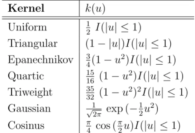
1.1 Kernel functions . . . 14 1.2 Estimating an additive model using the backfitting

al-gorithm . . . 23 1.3 General local scoring algorithm. . . 28 1.4 Eigenvalues and tolerance of independent variables . . 30

2.1 Backfitting algorithm for nonlinear regression with op-timal scaling . . . 46 2.2 Boston Housing dataset . . . 47 2.3 Eigenvalues of the correlation matrix and tolerance of

the predictors . . . 48 2.4 Regression coefficients of the model which considers only

numerical transformations of all predictors . . . 49 2.5 Coefficients of the model considering a nominal spline

transformation (2,2) for predictor AGE and numerical transformation for all the other predictors . . . 51 2.6 Coefficients of the model considering a nominal

trans-formation for predictor AGE and INDUS and numerical transformation for all the others predictors . . . 55

(10)

2.7 Eigenvalues of the correlation matrix and tolerance val-ues before and after applying nominal transformations on AGE and INDUS . . . 58 2.8 Coefficients of the model considering a nominal

formation for AGE and INDUS, and an ordinal trans-formation for LSTAT (numerical transtrans-formation for all others predictors) . . . 59

3.1 Eigenvalues and tolerance for simulated dataset, 5 pre-dictors . . . 66 3.2 EPE and APE and respective standard errors for

dif-ferent boosted models, simulation with five predictors . 67 3.3 Eigenvalues and tolerance for simulated dataset, 5

pre-dictors . . . 68 3.4 Eigenvalues and tolerance for simulated dataset, 13

pre-dictors . . . 69 3.5 EPE and APE and respective standard deviation for

different boosted models, simulation with thirteen pre-dictors . . . 70 3.6 Eigenvalues and tolerance for simulated dataset, 13

pre-dictors . . . 71 3.7 Real dataset, data description . . . 73 3.8 Eigenvalues of the correlation matrix and tolerance

val-ues, real dataset . . . 74 3.9 EPE and APE and respective standard deviation for

different boosted models, real data . . . 75 3.10 Eigenvalues and tolerance values before and after each

(11)

List of Figures

1.1 Example of regressogram: Prestige data fromRpackage car. The number of bins is 10 and binwidth is equal to 0.96. . . 9 1.2 Example of symmetric running-mean: Prestige data

fromR package car. Span is equal to 0.088 (k = 4). . . 11 1.3 Example of symmetric running-line: Prestige data from

R package car. Span is equal to 0.088 (k = 4). . . 13 1.4 Example of Gaussian Kernel estimator: Prestige data

fromR package car. . . 15 1.5 Example of cubic spline estimator: Prestige data from

R package car. Smoothing parameter is 0.86 . . . 17 1.6 Example of Lowess estimator: Prestige data from R

package car. . . 18 1.7 Additive model that relates the outcome variable to the

predictors. Each plot represents the contribution of a term to the additive predictor. The ‘y-axis’ label repre-sents the expression used to specify the corresponding contribution in the model formula. . . 32

(12)

1.8 True function of the effect of predictorxon the outcome variable . . . 33

2.1 Standardized partial linear residuals versus ized predictor AGE. The line represents the standard-ized nominal transformation of predictor AGE . . . 52 2.2 Standardized partial linear residuals versus

standard-ized transformation of predictor AGE. . . 53 2.3 Standardized partial linear residuals versus

standard-ized predictors, AGE and INDUS. The lines in these plots represent the standardized nominal transforma-tions of AGE and INDUS, respectively. . . 56 2.4 Standardized partial linear residuals versus

standard-ized transformations of predictors AGE and INDUS. . . 57 2.5 Standardized partial residuals versus standardized

pre-dictors, AGE, INDUS and LSTAT. The lines in these plots represent, respectively, the standardized nominal transformations for predictors AGE and INDUS, and standardized ordinal transformation for predictor LSTAT. 60 2.6 Standardized partial residuals versus standardized

(13)

Introduction

This monograph is focused on nonparametric nonlinear regression and additive modeling.

Regression analysis is a central method of statistical data analysis. Linear regression concerns the conditional distribution of a dependent variable, Y, as a function of one or more predictors, or independent variables. The main characteristics of this model are its parametric form and the hypothesis that the underlying relationship between the outcome and the predictors is linear. For this reason this method is often inappropriate to model this relationship when it is characterized by complex nonlinear patterns and it can fail to capture important features of the data.

In such cases, nonparametric regression, which allows to determine the functional form between the dependent variable, Y, and the explica-tive variables by the data themselves, is more suitable. Hence, non-parametric methods become increasingly popular and apply to many area of research and practical problems. These methods show a great flexibility compared to parametric ones, but they also present an im-portant drawback known as curse of dimensionality, which involves

(14)

that the precision of the estimates obtained via these methods is in inverse proportion to the number of explicative variables that are in-cluded in the model.

To overcome this problem Generalized Additive Models (GAM) were introduced. GAMs are based on the assumption that the conditional value of the outcome variable can be expressed as the sum of a certain number of univariate nonlinear functions, one for each predictor that is included in the model. One major concern to the use of the GAM is, therefore, when concurvity is present in the data. Concurvity can be defined as the presence of nonlinear dependencies among transfor-mations of the explanatory variables considered in the model. One of the most common case of concurvity directly follows from the presence of collinearity among the untransformed predictors. In the context of generalized additive models the presence of concurvity leads to biased estimates of the model parameters and of their standard errors.

For such reasons we explore an alternative class of models,CATREG, based on the Regression with Transformation approach, applying the optimal scaling methodology as presented in the Gifi system. When we use this class of models in the presence of collinearity among un-transformed predictors, applying nonlinear transformations through optimal scaling implies that interdependence among these predictor decreases.

Moreover in the framework of nonlinear regression with optimal scal-ing, we follow the approach proposed by Meulman (2003) of consid-ering models in which, applying the basic idea of a forward stagewise boosting procedure, we introduce in the model nonlinear prediction components in a sequential way with the aim of improving the predic-tive power of the model itself. We call this approach the Generalized Boosted Additive Model (GBAM).

(15)

Introduction

This monograph is structured as follows.

In first chapter we explore nonparametric regression models and their methodological framework. This chapter deals also with (Generalized) Additive Models, focusing on their advantages and limitations. The second chapter is about nonlinear regression with optimal scal-ing and its theoretical context. In this chapter we focus on the fact that when collinearity is present in the data, applying nonlinear trans-formations via optimal scaling on the predictor results in decreasing the interdependence among them and we present some illustrations through real data analysis.

The third chapter is about Generalized Boosted Additive Models. Af-ter presenting their theoretical background, we show, through the use of simulations and the analysis of a real dataset, that in case of collinearity among predictors, which implies the presence of approxi-mate concurvity among nonlinear transformations of these explicative variables, the proposed strategy leads to a solution that is a huge improvement compared to the linear model in terms of expected pre-diction error. At the same time, the use of prepre-diction components in GBAM has the advantage of reducing the computational burden by decreasing the number of iterations required in each step of the procedure significanlty.

(16)

(17)

Chapter 1 Generalized Additive Models

1.1 Introduction

Regression analysis is a central method of statistical data analysis. By extension and generalization, it provides the basis for much of applied statistics.

Regression analysis concerns the conditional distribution of a response, or dependent variable, Y, as a function of several predictors, or inde-pendent variables. The object is to estimate the the regression coeffi-cients {βj}p₁ of the model.

The expected value of the dependent variable is, for this reason, ex-pressed as a linear combination of the predictors and the parameters in the model.

E(Y|x) =β1x1+β2x2+...+βpxp =xTβ (1.1)

where E(y|x) is the expected value of y and depends on the partic-ular realization of the vector xT _{= (}_x

1, x2, ..., xp)T. If we define as

(18)

expected value E(Y|x):

=Y −E(Y|x) (1.2)

we can write the model as:

Y =xTβ+ (1.3)

The main characteristics of this model are the parametric form (i.e. the regression function is completely determined by the unknown pa-rameters, βj) and the hypothesis of a linear relationship between the

dependent variable and the predictors.

Given a sample, the estimation of the parameters in the model is usually obtained by least squares.

1.2 Nonparametric Regression

If we suppose that the relationship between the dependent variable and the predictors is completely described by a generic functionm(·), which can be either linear or nonlinear, the regression model can be expressed in the following way:

E(Y|x1, x2, ..., xp) = m(x1, x2, ..., xp) (1.4)

The model in equation (1.4) is known as nonlinear regression.

The object of nonparametric regression is to estimate the regres-sion function m(·) directly, rather than to estimate parameters. Most methods of nonparametric regression implicity assume that m(·) is a smooth, continuous function.

The precision of the estimates obtained via this kind of models is in inverse proportion to the number of predictors which are included in the model. This problem is known as curse of dimensionality [2, 29]. The relationship between the dependent variable and the independent

(19)

1.2. Nonparametric Regression

variables can be graphically represented by a surface whose dimensions depend on the number of predictors that are included into the model. In general smoothing techniques used in nonparametric regression are based on the idea of locally averaging the data to obtain an estimate of the mean response curve.

Suppose that we want to estimate the following model:

E[Y|(x1, x2)] =m(x1, x2)

and suppose that m(·) is a smooth function.

These smoothing techniques give an estimate of the functionm(·) in an arbitrary point (x1 =s, x2 =e) using alocal weighted average of the

values of the dependent variable, Y, that correspond to some values of the independent variables that are situated in a small neighborhood of the arbitrary point that has coordinates equal to (s, e). This weighted average is characterized by a proximity concept: the values ofY receive a higher weight if the correspondent couple of values of x1 and x2

are closer to the point (s, e), otherwise they receive a lower weight. The outcome of this non-parametric model characterized by only two predictors will be the approximation of a scatterplot in a 3-dimensional space with a surface. Formally this local weighted average procedure can be defined as:

ˆ m(x) = 1 n n X i=1 wi(x)Yi (1.5)

where w denotes a sequence of weights that may depend on the com-plete vector xT. Section 1.2 describes some of the most important smoothing methods that fall into the class of linear smoothers.

1.2.1 Smoothing methods

According to the definition in [55], an estimator ˆfn of f is a linear

(20)

such that ˆ fn(x) = n X i=1 li(x)Yi (1.6)

If we define the vector of fitted values as ˆf = ( ˆfn(x1), ...,fˆn(xn))T,

where y= (Y1, ..., Yn)T, then follows that:

ˆ_f ₌_Sy _(1.7)

where S is the n×n smoothing matrix, whose i-th row is l(xi)T, the

effective Kernel for estimating f(xi), contains the weights given to

eachYi in forming the estimate ˆfn(xi). Note that the smoother matrix,

S, depends on the dependent variables, as well as on the smoother, but not on Y. The trace of the smoothing matrix represents the degrees of freedom of the linear smoother. The simplest linear smoother is the Regressogram [77]. Suppose that all the predictor values are included in the interval (a, b),a ≤xi ≤b,i= 1, ..., n. If we divide this

interval into m equally spaced bins, bj, j = 1, ..., m, and define

ˆ

fn(x) =

X

i:xi∈bj

li(x)Yi, f or x ∈bj, (1.8)

whereli(x) = _n1_j ifxi ∈bj, 0 otherwise, andni is the number of points

included into bj, then the estimate ˆfn is a step function obtained by

averaging the Yi in each bin (note that in this case we are assigning

equal weights to each observation that falls into a certain bin). The binwidthh = (b−_ma) controls the smoothness of the estimate (the higher the h, the smoother the estimate).

A way to improve the estimate obtained from the regressogram is to consider overlapping regions, instead of disjoint and exhaustive regions. This is the main idea of two other simple smoothers, the

(21)

1.2. Nonparametric Regression ● ● ● ● ● ● ● ● ● ● ● ● ● ● ● ● ●● ● ● ● ● ● ● ● ● ● ● ● ● ● ● ● ● ● ● ●_● ● ● ● ● ● ● ● ● ● ● ● ● ● ● ● ● ● ● ● ● ● ● ● ● ● ● ● ● ● ● ●● ● ● ● ● ● ● ● ● ●● ● ● ● ● ● ● ● ● ●● ●● ● ● ● ● ● ● ● ● ● ● 6 8 10 12 14 16 20 40 60 80 education prestige

Figure 1.1: Example of regressogram: Prestige data fromR package

(22)

Therunning-meansmoother, also known asnearest neighborhood, produces a fit at the target point x by averaging the data points in a

neighborhood Ni aroundx. Conversely to the regressogram, the width

of the neighnorhood is variable and not fixed. In other words, the val-ues of the dependent variable, Y, that are considered to calculate the mean, are those which correspond to the k values of the independent variable X that are closer to the target point. More formally,

ˆ f(xi) = 1 n X j∈N(xi) Yj. (1.9)

The neighborhoods that are commonly used are symmetric nearest neighborhoods consisting of the nearest 2k+ 1 points:

N(xi) = {max(i−k,1), ..., i−1, i, i+ 1, ..., min(i+k, n)}. (1.10)

Therefore thek parameters control the smoothness of the estimate: a large value of k will produce smoother curves, whereas a small value will produce more jagged estimates. We set w = (2k_n+1), which repre-sents the proportion of points that are included in each neighborhood. The proportion w is called the span and controls the smoothness of the estimate (the larger the span, the smoother the functions). Even though this smoother is simple in practice, it tends to be wiggly and to flatten out trends near the endpoints, so it can be severly biased.

A simple generalization of the running-mean smoother is the running-line smoother. This smoother fits a line by ordinary least squares to the data in a symmetric nearest neighborhoodNi around eachxi. The

estimated smooth at xi is the value of the fitted line at xi:

ˆ

f(xi) = ˆα(xi) + ˆβ(xi)xi, (1.11)

where ˆα(xi) and ˆβ(xi) are the coefficients obtained by ordinary least

(23)

Figure 1.2: Example of symmetric running-mean: Prestige data from

(24)

the number of points included in the neighborhood, as in the previous case, determines the shape of the estimate. Moreover, also in this case the span w = (2k_n+1) indicates the proportion of points in each neighborhood. In the extreme case, if w = 2, each neighborhood contains all the data, the running-line smoother is the least square line, while if w = 1_n, each neighborhood contains just one data point and the smoother interpolates the data. The running-line smoother is considered to be an improvement over the running-mean because it reduces the bias near the endpoints. But also this smoother, like the other examined up to this point, can produce jagged curves, because it assigns equal weights to all the points included in a given neighborhood and zero weight to points outside the neighborhood.

Differently from the smoothers presented up to this point, Ker-nel smoothers refine moving average smoothing through the use of a weighted average. In other word, they explicitly use a specified set of weigths Wi, defined by the kernel, to obtain an estimate at each

target value: they describe the shape of the weight function by a den-sity function with a scale parameter, h, that adjusts the size and the form of the weights near the target point. The kernel is a non-negative symmetric real integrable function K which satisfies:

Z +∞ −∞

K(u)du= 1.

More formally, the estimate given by a generic Kernel smoother can be written as: ˆ fh(x) = P iwiyi P iwi (1.12)

The distance from the target point is

di =

xi−x

(25)

Figure 1.3: Example of symmetric running-line: Prestige data from

(26)

and it measures the scaled and signed distance between thex-value for thei-th observation and the target pointx. The scale factorh con-trols the bin width and, so, the smoothness of the estimate. Within each bin, the set of weights results from applying the kernel function to the distances calculated for the observations in the bin,wi =K

_x_i−x h

. Then, these weights are used to calculate the local weighted average in equation (1.12). In Table 1.1 we show several kinds of kernel function which are commonly used [49]. The value u in Table 1.1 is equal to

u= (X−Xi)/h and I(·) is the indicator function.

The kernel specifies how the observations in the neighborhood of the

Kernel k(u) Uniform 1₂ I(|u| ≤1) Triangular (1− |u|)I(|u| ≤1) Epanechnikov 3₄(1−u2)I(|u| ≤1) Quartic 15₁₆ (1−u2)I(|u| ≤1) Triweight 35₃₂ (1−u2)2I(|u| ≤1) Gaussian √1 2π exp (− 1 2u 2₎ Cosinus π₄ cos (π₂u)I(|u| ≤1)

Table 1.1: Kernel functions

target point, x, contribute to the estimate in that point. Whatever the weighting function is, the weights must have certain properties: (1) they must be symmetric with respect to the target point; (2) they must be positive, and (3) they must decrease from the target point to the bin boundaries.

Even though the kernel smoother represents an improvement with re-spect to the simple moving average smoother, it has a drawback: the

(27)

mean cannot be considered as an optimal local estimator, and using a local regression estimate instead of a local mean produces a better fit.

● ● ● ● ● ● ● ● ● ● ● ● ● ● ● ● ● ● ● ● ● ● ● ● ● ● ● ● ● ● ● ● ● ● ● ● ● ● ● ● ● ● ● ● ● ● ● ● ● ● ● ● ● ● ● ● ● ● ● ● ● ● ● ● ● ● ● ● ● ● ● ● ● ● ● ● ● ● ● ● ● ● ● ● ● ● ● ● ● ● ● ● ● ● ● ● ● ● ● ● ● ● 6 8 10 12 14 16 20 40 60 80 education prestige bandwidth = 2 bandwidth = 5

Figure 1.4: Example of Gaussian Kernel estimator: Prestige data

from Rpackage car.

Spline smoothers represent the estimate as a piecewise polyno-mial of a fixed order. Regions that define the pieces are separated by a sequence of knots (or breakpoints) and the piecewise polynomials are forced to joint smoothly in correspondence to these knots. For a given set of knots, the estimate is computed by multiple regression on a set of basis vectors which are the basis functions representing the

(28)

particular family of piecewise polynomials, evaluated at the observed values of the predictors. There are several types of spline smoothers: regression splines, cubic splines, B-splines, P-splines, natural splinse and smoothing splines, and many others. In the simplest regression splines, the piecewise functions are linear. In practice, we fit separate regression lines within the regions between the knots, and the knots tie together the piecewise regression fits. Also in this case, splines are a local model with local fits between the knots instead of within bins, and allow us to estimate the functional form from the data. Like in other smoothing functions we must make several decisions: we need to decide the degree of the polynomial for the piecewise function, the number of knots, and their placement. The evaluation of all the dif-ferent spline smoothers is far beyond the aim of this monograph, for a wider coverage refer to [4, 17, 20, 55].

The locally weighted running-line smoother (LOWESS) [12] combines the local nature of running-line smoother and the smooth weights of the kernel smoother. The idea is to start with a local polynomial least-squares fit computed in different steps. In the first step the k nearest neighbors of the target point, x, are identified. Then, we compute the distance of the furthest near-neighbor from x, ∆(x). The weightswi are assigned to each point in the neighborhood

using the tri-cube weight function

W kx−xik ∆(x) , (1.14) where W(u) = ( (1−u3₎3 _for ₀_≤_{u <}_1; 0 otherwise. (1.15)

Then, the estimate is the fitted value at x from the weighted least-squares fit of ytox in the neighborhood using the computed weights.

(29)

1.2. Nonparametric Regression ● ● ● ● ● ● ● ● ● ● ● ● ● ● ● ● ● ● ● ● ● ● ● ● ● ● ● ● ● ● ● ● ● ● ● ● ● ● ● ● ● ● ● ● ● ● ● ● ● ● _● ● ● ● ● ● ● ● ● ● ● ● ● ● ● ● ● ● ● ● ● ● ● ● ● ● ● ● ● ● ● ● ● ● ● ● ● ● ● ● ● ● ● ● ● ● ● ● ● ● ● ● 6 8 10 12 14 16 20 40 60 80 education prestige

Figure 1.5: Example of cubic spline estimator: Prestige data from R

(30)

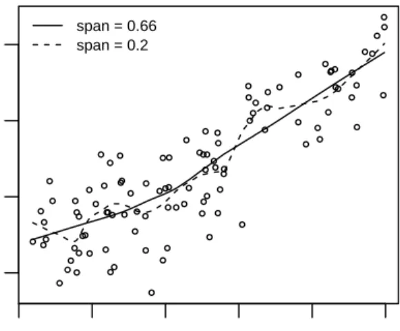
● ● ● ● ● ● ● ● ● ● ● ● ● ● ● ● ● ● ● ● ● ● ● ● ● ● ● ● ● ● ● ● ● ● ● ● ● ● ● ● ● ● ● ● ● ● ● ● ● ● _● ● ● ● ● ● ● ● ● ● ● ● ● ● ● ● ● ● ● ● ● ● ● ● ● ● ● ● ● ● ● ● ● ● ● ● ● ● ● ● ● ● ● ● ● ● ● ● ● ● ● ● 6 8 10 12 14 16 20 40 60 80 education prestige span = 0.66 span = 0.2

Figure 1.6: Example of Lowess estimator: Prestige data fromR

(31)

1.2.2 Span selection and the Bias-Variance

Trade-off

A smoother is considered effective if it produces a small prediction error, usually measured by the Mean Squared Error (MSE).

M SE( ˆfh(x)) =E ˆ fh(x)−f(x) 2 =Bias2( ˆfh(x)) +V ar( ˆfh(x)), (1.16) where Bias=Ehfˆh(x)−f(x) i (1.17) and V ar( ˆfh(x)) =E ˆ fh(x)−Efˆh(x) 2 . (1.18)

We can see that the bandwidth controls the trade-off between the squared bias and the variance: when h is large, the squared bias is large but the variance is small and viceversa. Intuitively, when the size of the local neighborhood is small this neighborhood contains few observations and so the estimate closely approximates f. This results in a small bias of the ˆfh(x). However, since there are only few

obser-vations in the neighborhood, the variance of the estimate is large. The smoothing parameter, from this point on indicated asλ, can be chosen by visual trial and error, picking a value that balances smooth-ness against the fit of the model.

Intuitively, a good smoothing parameter should produce a small aver-age mean squared error:

ASE( ˆfλ) =N−1 N X i=1 M SE( ˆfλ(xi)) = N−1 N X i=1 ˆ fλ(xi)−f(xi) 2 , (1.19)

(32)

but this quantity is not defined because f is an unknown function which has to be estimated. A good estimator for the ASE is the cross-validation score: CV(λ) = N−1 N X i=1 ˆ f_λ−i(xi)−yi 2 , (1.20)

where ˆf_λ−i(xi) is the fitted value at point xi if we use all the data

points except (xi, yi).

The cross-validation procedure selects the λ that minimizes the score in equation (1.20). Moreover, for linear smoother the CV score can be simplified as,

CV(λ) =N−1 N X i=1 ˆ fλ(xi)−yi 1−Sii !2 (1.21)

where Sii is the i-th diagonal element of the smoother matrix S,

see [55] for details. Repeating this procedure for different values of the smoothing parameter will suggest a value that minimizes the cross-validation estimate. Often, Generalized cross-validation, first pro-posed by [86] is used, whereSiiis replaced by its average valuetr(S)/N

and, for this reason, easier to compute.

1.2.3 Curse of dimensionality

With increasing dimensionality p, these techniques suffer under the curse of dimensionality [2]. The relationship between the dependent variable and the independent variables can be graphically represented by a surface whose dimension depends on the number of predictors included in the model. The use of nonparametric estimators, which are for sure more flexible compared to those used in parametric mod-els, is for this reason often used with complementary methods for the

(33)

1.3. Additive Models

reduction of dimensionality. This means that if we define a local neigh-borhood over which we want to average the data to obtain an estimate, then this neighborhood is most likely empty (i.e. has no observations in it). Vice versa, if we choose the neighbourhood such that it is not empty, then the estimate will be no longer local. But even if we could estimate the smooth function reliably, it is not clear how we can vi-sualise the response curve (surface) for large number of predictors to gain the insight that we are looking for.

To overcome these two problems a class of models have been proposed known as (generalized) additive models [50, 76]. Here, we do not as-sume that the response curvef is a smoothp-variate function. Rather, the assumption is that f can be written as the sum of p univariate functions each of which has one predictor as argument.

1.3 Additive Models

A very useful generalization of the ordinary multiple regression

yi =α+βxi+i,

is the class of additive models:

yi =α+f(x1,i) +...+f(xp,i) +i. (1.22)

The form of the multiple regression model is relaxed: as in linear regression, the additive regression model specifies the expected value of Y as the sum of separate terms for each predictor, but now these terms are assumed to be smooth functions of the independent vari-ables. Even in this case the model might have component functions with one or more dimensions, as well as categorical variable terms and their interactions with continuous variables. Obviously we assume that

(34)

otherwise there will be a free constant in each of the functions. A substantial advantage of the additive regression model respect to nonparametric regression is that it eliminates the curse of dimension-ality, as it reduces to a series of two-dimensional partial regression problems.

Moreover, since each variable is represented in a separate way the model has another important interpretative feature which is common to the linear model: the variation of the fitted response surface, hold-ing all predictors constant except one, does not depend on the values of the other predictors. In other words, as each partial regression problem is a two-dimensional problem, we can estimate separately the partial relationship between the dependent variable and each predictor.

The model is fitted by iteratively smoothing partial residuals in a process known as backfitting, which is a block1 _Gauss-Seidel

pro-cedure for solving a system of equations. The idea of the backfitting algorithm goes back to Friedman and Stuetzle [38], who used it for pro-jection pursuit regression, Breiman and Friedman [6], who employed it in their Alternating Conditional Expectation algorithm (ACE) and Young, De Leeuw and Takane [92], who used it in their alternating least squares algorithm (CORALS).

We can notice that in the additive model,

E " Y −α− p X j6=k fj(xj)|xk # =fk(xk) (1.23)

holds for anyk, 1 < k < p. This suggests the use of an iterative algorithm to calculate the fj.

Given a set of initial estimates{α,ˆ fˆj}, we can improve these estimates

iteratively (i.e. looping over j = 1, ..., p ) by calculating the partial

1_{Backfitting constitutes a block Galuss-Seidel procedure for the fact that}

(35)

1.3. Additive Models

residuals from the observations{xj, Yi}. Considering the partial

resid-uals r[1]_i =yi−αˆ− p X l6=k fl(xil), (1.24)

and smoothingr[1] againstxj to update the estimate ˆfi.

The backfitting algorithm for Additive model is sketched in Table 1.2.

1. Set the counterk to zero. Initialise ˆα and ˆfi as

ˆ

α= ¯y= 1_nPn

i=1yi

ˆ

fj(xj) = 0 for j= 1, ..., p and fori= 1, ..., n

2. For j= 1, ..., p do:

Calculate partial residuals: ri=yi−αˆ−Pp_l₌₁ l6=j

ˆ

fl(xil), i= 1, ..., n

Update the jth smooth function: ˆfj(·) =Sj(wi, xij)r

3. Check for convergence.

If the algorithm has not converged yet, set k=k+ 1 and go to 2. Else return.

Table 1.2: Estimating an additive model using the backfitting

algo-rithm

Thefjs are arbitrary univariate and smooth functions, one for each

predictor.

A two-dimensional plot is sufficient to examine the estimated partial regression function ˆfj relating y to xj holding the other explanatory

variables constant. This means that interpretation of additive regres-sion models is relatively simple, assuming that the additive model ad-equately captures the dependence of Y on the independent variables.

(36)

In other words, the backfitting algorithm solves the following system of estimating equations:      I S1 S1 · · · S1 S2 I S2 · · · S2 .. . ... ... . .. ... Sp Sp Sp · · · I           f1 f2 .. . fp      =      S1Y S2Y .. . SpY      (1.25)

where Iis a n×n unit matrix. In a short form we can write:

Pf=QY (1.26)

1.4 Generalized Additive Models

Generalized additive models represent a flexible extension of general-ized linear models [59], allowing non-parametric smoothers in addition to parametric forms combined with a range of link functions and pro-vide one way to extend the additive model. More specifically, the effects of the predictors are assumed to be linear in the parameters, but the distribution of the response variable, as well as the link be-tween the predictors and this distribution, can be quite general. At least two other estensions have been proposed: Friedman and Stue-zle [38] introduced Projection Pursuit Regression and Breiman and Friedman [6] introduced Alternating Conditional Expectation.

A generalized linear models is specified by three components:

a random component: we specify the distribution of the response variable and we assume that it comes from exponential family density, f(Y, θ, φ) = exp Y θ−b(θ) a(θ) +c(Y, φ) , (1.27)

(37)

1.4. Generalized Additive Models

which includes many distributions that are useful for practival modelling, such as the Poisson, Binomial, Gamma and Normal distribution. The canonical parameterθ represents the location, while the dispersion parameter φ represents the scale of the ex-ponential distribution taken into account. Moreover ai(φ), (θi)

and c(yi, φ) are known functions. Generally ai(φ) has the form ai(φ) = _wφ₀, where w0 is a known prior weight, usually equal to

1.

a systematic component: we assume that the expected value of the response variable is related to the set of covariates by a linear predictor,

η =βX.

a link function that describes how the expected value of the response variable is linked to covariates through linear predictor,

g(µ) =η.

Estimation and inference with generalized linear models is based on the theory of maximum likelihood estimation. For a single observation the log-likelihood is:

logL(θi, φ, Yi) = Yiθi −b(θi) ai(φ) +c(Yi, φ) (1.28)

So for independent observations, the log-likelihood will beP

ilogL(θi, φ, Yi).

We can maximize this analytically and find an exact solution for the MLE, ˆβ, only if the response variable has a Gaussian density function, otherwise numerical optimization is required. McCullagh and Nelder [59] showed that the optimization is equivalent to itera-tively reweighted least squares (IRWLS), which turns out to be equivalent to Fisher’s method of scoring, which is simply the Newton-Raphson method with the Hessian replaced by its expected value.

(38)

Given a starting estimate of the parameters ˆβ, we calculate the estimated linear predictor ˆηi = x0iβˆ and use that to obtain the fitted

values ˆµi = g−1( ˆηi). Then we calculate, using these quantities, the

working dependent variable as

zi = ˆηi+ (yi−µˆi) ∂ηi ∂µi (1.29)

The rightmost term in (1.29) is the derivative of the link function eval-uated at the initial estimate. Next we calculate the iterative weights as: wi = 1 b00(θi) ∂ηi ∂µi 2 (1.30)

where b00(θi) is the second derivative of b(θi) evaluated at the starting

estimate assuming ai(φ) = φ. This weight is inversely proportional

to the variance of the working dependent variable, given the current estimate of the parameters, with proportionality factor equal to φ. From this point on we obtain an updated estimate of theβ, regressing the working dependent variablezi on the predictors, using the weights wi. In other words, we calculate the weighted least-square estimate

ˆ

β = (X0WX)−1X0Wz (1.31)

where X is the model matrix, W is a diagonal matrix of weights (with entries wi) and z is the response vector, with entries zi. This

procedure is repeated until two successive estimates change less than a pre-specified small amount.

The linear predictor in GLM, η =βX, specifies that the indepen-dent variables act in a linear way onto the response. According to [50], a more general model can be:

η=α+

p

X

i

(39)

1.5. Degeneracy in GAMs: concurvity

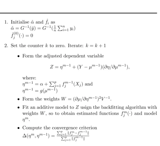
where f(·)s are smooth functions. As in the GLM the estimates are found by regressing repeatedly the adjusted dependent variable z on the predictors. In this ‘smooth’ version of the model in (1.32) it is pos-sible to estimate thef(·) by repeatedly smoothing the adjusted depen-dent variable onX. The authors called this procedure local scoring. A general local scoring algorithm, as reported in [50], is sketched in Table 1.3. As shown in Buja, Hastie and Tibshirani [8], the backfit-ting algorithm will always converge. Being the local scoring simply a Newton-Raphson step, if the step size optimization is performed, it will converge as well. Note moreover that the convergence is moni-tored by a change in the fitted functions rather than in the deviance. Because the deviance is penalized, as analitically shown in [55], it can increase during the iterations, especially when the starting functions are too rough.

1.5 Degeneracy in GAMs: concurvity

As the term collinearity refers to linear dependencies among the in-dependent variables, the term concurvity [8] describes the nonlinear dependencies among the predictor variables. In this sense, as collinear-ity results in inflated variance of the estimated regression coefficients, the result of the presence of concurvity will lead to instability of the estimated coefficients in GAM. As mentioned in [8]:

“Concurvity boils down to collinearity of (nonlinear) transforms of predictors”.[8], p484

Exact concurvity is defined as the existence of a nonzero solution,

(40)

equa-1. Initialise ˆα and ˆfi as ˆ α=G−1(¯y) =G−1(_n1 Pn i=1yi) ˆ f_j(0)(·) = 0

2. Set the counterkto zero. Iterate: k=k+ 1 Form the adjusted dependent variable

Z =ηm−1+ (Y −µm−1)(∂η/∂µm−1), where: ηm−1=α+Pp j=1f m−1 j (Xj) and ηm−1=g(µm−1)

Form the weightsW = (∂µ/∂ηm−1)2V−1.

Fit an additive model toZusign the backfitting algorithm with weights W, so to obtain estimated functions fm

j (·) and model

ηm.

Compute the convergence criterion ∆(ηm, ηm−1) = Pp j=1kfjm−f m−1 j k Pp j=1kf m−1 j k

Repeat step 2 until the convergence criterion is below some small threshold.

(41)

1.5. Degeneracy in GAMs: concurvity tions:      I S1 S1 · · · S1 S2 I S2 · · · S2 .. . ... ... . .. ... Sp Sp Sp · · · I           g1 g2 .. . gp      =      0 0 .. . 0      (1.33)

If such g exists and f = (f1, f2, ..., fp)T is a solution of the system

of normal equations in (1.25), then the system will have an infinite number of solution because for any c also f+cg will be a solution. In other words, the concurvity space of (1.26) is the set of additive functions g(x) =P

gk(xk) such that Pg= 0.

As demonstrated in [55], concurvity is present when the spaces spanned by the eigenvectors of the smoothing matrices are linearly dependent. As demonstrated in [8], if we consider symmetric smoothers, for ex-ample cubic spline smoothers, exact concurvity will be present only in case of a perfect collinearity among the untransformed predictors.

Note that, in contrast to the linear regression framework where collinearity implies that the solution of the equation system cannot be found unless the data matrix is transformed in a full rank matrix or a generalized inverse is defined, the presence of concurvity does not imply that the backfitting algorithm will not converge. It has been demonstrated that backfitting algorithm will always converge to a solution. In case of concurvity the starting functions will determine which solution of (1.25) will be the final solution. While exact con-curvity is highly unlikely, except in the case of symmetric smoothers with eigenvalues [0,1], since it can only derive from an exact collinear-ity among the original predictors, approximate concurvcollinear-ity is of prac-tical concern, because it can lead to upwardly biased estimates of the parameters and to the underestimation of their standard errors.

(42)

1.6 An illustration

In this section we try to illustrate the effects of strong concurvity in fitting a generalized additive model with a simulated example. As mentioned before, concurvity is present in the data when the predic-tors are collinear. We simulate a total of n = 200 observations. We simulate three predictors (x, z and t) independently from a uniform distribution U[0,1]. The forth predictor, g is generated as:

g = 3×x3+N(0,0.0001) to show strong concurvity with predictor x.

Eigenvalues Tolerance

x 1.93871 0.14917

t 1.07470 0.97570

z 0.90923 0.98721

g 0.07736 0.14856

Table 1.4: Eigenvalues and tolerance of independent variables

In Table 1.4 we report the eigenvalues of the correlation matrix of the four predictors and corresponding values of the tolerance. Obvi-ously, there is a strong relation between x and g. Furthermore, we generate the outcome variable, y, as:

y= 3×e−x+ 1.3×x3+t+N(0,0.01),

So, yis function only of x and t. Now we fit a generalized additive model on these data using the R package gam created by Hastie and Tibshirani (smoothing parameters estimates are determined via cross validation).

(43)

1.6. An illustration

Call: gam(formula = y ~ -1 + s(x, df = 5) + s(t, df = 1) + s(z, df = 2) + s(g, df = 1), family = gaussian, data = datas)

Deviance Residuals:

Min 1Q Median 3Q Max

-2.64432 -0.66797 0.02713 0.68381 2.38037

(Dispersion Parameter for gaussian family taken to be 0.9417) Null Deviance: 2166.579 on 200 degrees of freedom

Residual Deviance: 177.984 on 189.0097 degrees of freedom AIC: 568.2313

Number of Local Scoring Iterations: 4

DF for Terms and F-values for Nonparametric Effects

Df Npar Df Npar F Pr(F) s(x, df = 5) 1 4 19.2320 2.743e-13 *** s(t, df = 1) 1 0 0.2410 0.04080 * s(z, df = 2) 1 1 1.5496 0.21474 s(g, df = 1) 1 2 6.5943 0.00178 ** ---Signif. codes: 0 ´S***ˇS 0.001 ´S**ˇS 0.01 ´S*ˇS 0.05 ´S.ˇS 0.1 ´S ˇS 1

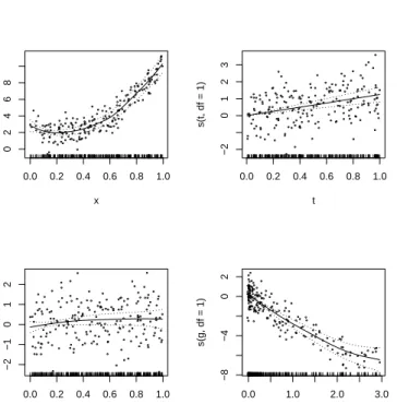
The results obtained above clearly show that the nonparametric effects for variables x and g are significantly different from zero. This arises only from the concurvity between predictors xand g. In Figure 1.7 we show the graphical representation of the model we fit.

Moreover, in Figure 1.8 we show the effect of the true function

(44)

● ● ● ● ● ● ● ● ● ● ● ● ● ● ● ● ● ● ● ● ● ● ● ● ● ● ● ● ● ● ● ● ● ● ● ● ● ● ● ● ● ● ● ● ● ● ● ● ● ● ● ● ● ● ● ● ● ● ● ● ● ● ● ● ● ● ●● ● ● ● ● ● ● ● ● ● ● ● ● ● ● ● ● ● ● ● ● ● ● ● ● ● ● ● ● ● ● ● ● ● ● ● ● ● ● ● ● ● ● ● ● ● ● ● ● ● ● ● ● ● ● ● ● ● ● ● ● ● ● ● ● ● ● ● ● ● ● ● ● ● ● ● ● ● ● ● ● ● ● ● ● ● ● ● ● ● ● ● ● ● ● ● ● ● ● ● ● ● ● ● ● ● ● ● ● ● ● ● ● ● ● ● ● ● ● ● ● ● ● ● ● ● ● ● ● ● ● ● ● 0.0 0.2 0.4 0.6 0.8 1.0 0 2 4 6 8 x s(x, df = 5) ● ● ● ● ● ● ● ● ● ● ● ● ● ● ● ● ● ● ● ● ● ● ● ● ● ● ● ● ● ● ● ● ● ● ● ● ● ● ● ● ● ● ● ● ● ● ● ● ● ● ● ● ● ● ● ● ● ● ● ● ● ● ● ● ● ● ● ● ● ● ● ● ● ● ● ● ● ● ● ● ● ● ● ● ● ● ● ● ● ● ● ● ● ● ● ● ● ● ● ● ● ● ● ● ● ● ● ● ● ● ● ● ● ● ● ● ● ● ● ● ● ● ● ● ● ● ● ● ● ● ● ● ● ● ● ● ● ● ● ● ● ● ● ● ● ● ● ● ● ● ● ● ● ● ● ● ● ● ● ● ● ● ● ● ● ● ● ● ● ● ● ● ● ● ● ● ● ● ● ● ● ● ● ● ● ● ● ● ● ● ● ● ● ● ● ● ● ● ● ● 0.0 0.2 0.4 0.6 0.8 1.0 −2 0 1 2 3 t s(t, df = 1) ● ● ● ● ● ● ● ● ● ● ● ● ● ● ● ● ● ● ● ● ● ● ● ● ● ● ● ● ● ● ● ● ● ● ● ● ● ● ● ● ● ● ● ● ● ● ● ● ● ● ● ● ● ● ● ● ● ● ● ● ● ● ● ● ● ● ● ● ● ● ● ● ● ● ● ● ● ● ● ● ● ● ● ● ● ● ● ● ● ● ● ● ● ● ● ● ● ● ● ● ● ● ● ● ● ● ● ● ● ● ● ● ● ● ● ● ● ● ● ● ● ● ● ● ● ● ● ● ● ● ● ● ● ● ● ● ● ● ● ● ● ● ● ● ● ● ● ● ● ● ● ● ● ● ● ● ● ● ● ● ● ● ● ● ● ● ● ● ● ● ● ● ● ● ● ● ● ● ● ● ● ● ● ● ● ● ● ● ● ● ● ● ● ● ● ● ● ● ● ● 0.0 0.2 0.4 0.6 0.8 1.0 −2 −1 0 1 2 z s(z, df = 2) ● ● ● ● ● ● ● ● ● ● ● ● ● ● ● ● ● ● ● ● ● ● ● ● ● ● ● ● ● ● ● ● ● ● ● ● ● ● ● ● ● ● ● ● ● ● ● ● ● ● ● ● ● ● ● ● ● ● ● ● ● ● ● ● ● ● ●● ● ● ● ● ● ● ● ● ● ● ● ● ● ● ● ● ● ● ● ● ● ● ● ● ● ● ● ● ● ● ●● ● ● ● ● ● ● ● ● ● ● ● ● ● ● ● ● ● ● ● ● ● ● ● ● ● ● ● ● ● ● ● ● ● ● ● ● ● ● ● ● ● ● ● ● ● ● ● ● ● ● ● ● ● ● ● ● ● ● ● ● ● ● ● ● ● ● ● ● ● ● ● ● ● ● ● ● ● ● ● ● ● ● ● ● ● ● ● ● ● ● ● ● ● ● ● ● ● ● ● ● 0.0 1.0 2.0 3.0 −8 −4 0 2 g s(g, df = 1)

Figure 1.7: Additive model that relates the outcome variable to the

predictors. Each plot represents the contribution of a term to the ad-ditive predictor. The ‘y-axis’ label represents the expression used to specify the corresponding contribution in the model formula.

(45)

1.6. An illustration 0.0 0.2 0.4 0.6 0.8 1.0 2.0 2.2 2.4 2.6 2.8 3.0 x1 3 e − x+ 1.3 x 3

Figure 1.8: True function of the effect of predictorx on the outcome

(46)

(47)

Chapter 2 Nonlinear categorical

regression

2.1 Introduction

In this chapter we will focus on the nonlinear categorical regression method,CATREG, which follows the Regression with Transformation approach, applying the optimal scaling methodology as presented in the so called ALSOS system [91] and in the Gifi system [39]. The ideas presented in this section are inspired by [64], in which the author argues that :

‘the particular transformations resulting from the re-gression problem would have a particular influence on the structure of the correlation matrix between the predictors after optimal scaling’ ( [64]; pp 498)

As we know, if the predictors in the linear regression model are inde-pendent, their correlation matrix is equal to the identity matrix with all eigenvalues equal to 1. In contrast, if collinearity is present, the

(48)

predictors are highly linearly related and this influences the size of the distribution of the eigenvalues and the value of the small eigenvalues. When the correlation among the predictors increases, the value of the smaller eigenvalues decreases.

In the presence of multicollinearity, nominal and ordinal transfor-mations obtained via optimal scaling linearize the relationship between the dependent variable and the predictors. In other words, the effect of these transformation is to decrease the interdependence among the predictors. This effect is stronger or weaker depending on the smooth-ness of the transformation itself (the smoother the transformation, the smaller the effect).

2.2 Optimal scaling

The optimal assignment of quantitative values to qualitative scales is an important development in multidimensional data analysis.

Optimal scaling represents a method to find an optimal transforma-tion to convert categorical variables into numeric data. This trans-formation process is known as ‘quantification’ [91]. In a regression framework, quantifications of the categorical variables are estimated in parallel with the estimation of the regression coefficients, via an alter-nating least squares procedure that maximizes the correlation between transformations of the dependent variable and the set of predictors. The result of this procedure is that the optimal scaling transforma-tions linearize the relatransforma-tionship between the dependent variable and the predictors. Numerical variables in this framework are treated as categorical ones, with a number of categories equal to the number of distinct values that the numeric variable presents. Of course optimal-ity must be interpreted in a wide sense because it is obtained always with respect to the particular data set and to a particular criterion that is optimized.

(49)

2.2. Optimal scaling

In the quantification process it is possible to preserve properties of the data in the transformations by choosing an appropriate optimal scaling level for the variables. Note that, when we use the term optimal scaling level, we refer to the level on which the variable is analyzed and not to the measurement level of the original variable, which can be different.

The properties of the data that can be preserved are grouping, ordering and equal relative spacing.

According to its measurement level a variable can have one, two or all of these properties. We can distinguish:

Variables with nominal measurement level: only grouping , i.e. the category values code the observations into the different classes

Variables with ordinal measurement level: grouping and order-ing, i.e. the category values code observations into the different classes and these classes are ordered .

Numeric variable: grouping, ordering and equal relative spacing To choose the scaling level, independent of the measurement level, we make the following distinction:

We use a nominal scaling level when we want just to maintain the class membership information, i.e. objects in the same group according to variable j obtain the same quantification in the transformed variable ϕj(xj).

xij =xi0_j ⇒ ϕ_j(x_ij) = ϕ_j(x_i0_j)

We use anordinal scaling level if a (categorical) variable contains order information on the objects and we want to preserve it in

(50)

the transformation. In this case xj and ϕj(xj) are related by a

monotonic function.

xij < xi0_j ⇒ ϕ_j(x_ij)≤ϕ_j(x_i0_j)

We use a numeric scaling level when we want to preserve all the properties. Note that if we use the numeric scaling level for a variable that is measured on a categorical level we treat the category values as numeric values, whereas if we use this scaling level for a numeric variable, this will result in a linear transformation to standard scores.

The scaling level is also related to the degrees of freedom of the transformation and to the fit of the model: transformations with less degrees of freedom will result in smoother transformations and worse fit and vice versa.

The transformation based on the nominal scaling level has the max-imum number of degrees of freedom, which is equal to the number of categories minus one. Otherwise, the transformation which derives from choosing the ordinal scaling level implies one more restriction on the quantification of the order of thee categories, so the number of degrees of freedom is equal to the number of categories with different quantified values minus one.

Among the different transformations two approaches are available:

step functions and spline functions.

Step functions are generally associated with categorical data, while

spline functions refer to continuous data. Moreover, a continuous vari-able can also be considered as a categorical varivari-able with a number of categories equal to the number of the objects. For this reason we need to limit the number of parameters we want to fit. For splines, the number of parameters is determined by the degree of the spline that we choose and the number of interior knots, thus we have to limit

(51)

2.2. Optimal scaling

both of them. In spline transformation case we consider monotonic and nonmonotonic spline.

Obviously the shape of the transformation is related to the number of degrees of freedom of the transformation itself. Transformations with more freedom will results in less smooth transformations and in a bet-ter fit and vice versa. In other words, this means that if we choose to preserve more properties of the data, using more restrictive transfor-mations, we lose something in terms of fit of the model.

2.2.1 Monotonic splines

Following [69], monotonic splines are a class of piecewise polynomi-als. A polynomial spline is a piecewise polynomial function defined on an interval [a, b] which is divided in a mesh consisting of points

a = ξ1 < ... < ξq = b. This mesh is also divided in subintervals

[ξj, ξj+1) within which the function is a polynomial piece of specified

order k.

Adjacent polynomial are required to join with a specified degree of smoothness at the boundaries of the subintervals. Smoothness is de-fined as the equality of the derivatives of the polynomial pieces at the joining points. In the common case, all orders of continuity, υj, are

specified as the degree k−1 of the polynomial. For example, ifk = 2 the spline consists of straightline segments that are required to match at the boundaries, whereas k = 3 the spline is a piecewise quadratic with matching first derivatives.

The domain and the continuity conditions are incorporated into the knot sequence,t={t1, ..., tn+k}, wherenrepresents the number of free

parameters (total degrees of freedom) that specify the spline function. This sequence has the following properties:

(52)

1.

t1 ≤...≤tn+k

2. For all i there exists aj such thatti =ξj.

3. The continuity characteristics are determined by:

t1 =...=tk =a and b=tn+1 =...=tn+k;

ti < ti+k for all i;

if ti =ξj and ti−1 < ξj then ti =...=ti+k−υj−1.

This means that the sequence of knots,t, is derived from the mesh by placing the number of knots at the boundary value according to the order of continuity desired. A spline of order k−1 is a polyno-mial at any point ξ and so it is determined by k free coefficients in the subinterval containing that point. But the continuity conditions impose υj linear equality constraints on the coefficients which define

adjacent polynomials. So the total degrees of freedom is equal to the value n.

The spline transformation can be computed by defining a set of basis splines, Mi(·|k, t), i = 1, ..., n such that any piecewise polynomial, f,

of orderk and associated sequence of knotst, can be represented as a linear combination f =P

biMi.

In the Monotonic spline family the set of basis spline is defined to be positive in (ti, ti+k) and zero elsewhere, and must comply with the

normalization propertyR Mi(x)dx= 1 [16]. So, eachMi has the

prop-erties of a probability density function over the interval [ti, ti+k]. The

monotonicity is assured by the nonnegativity of bi.

Because monotonic splines are nonnegative we can define integrated spline as:

Ii(x|k, t) =

Z x

L

(53)

2.3. Nonlinear regression with optimal scaling

where L is the lower limit of the domain of the spline. Since each

Mi is a piecewise polynomial of degree k −1, each Ii is a piecewise

polynomial of degree k.

For a simple knot sequence, for which tj ≤ x < tj +k for all x, the

I-spline Ii can be computed as:

Ii(x|k, t) =      0, i > j, Pj m=1(tm+k+1−tm)Mm(x|k+ 1, t)/(k+ 1), j−k+ 1≤i≤j, 1, i < j−k+ 1 (2.2)

2.3 Nonlinear regression with optimal

scal-ing

As mentioned before, in linear regression a dependent variable Y is predicted from a set of p independent variables X. The aim of the regression is to find a linear combination of X that is maximally cor-related with the dependent variable.

In terms of a least squares loss function we write:

L(β) =ky−βXk2 =ky−

J

X

j=1

βjxjk2 (2.3)

We assume that the predictors are normalized to have zero mean and sum of squares equal to one, so we do not need to fit an intercept. The analytic solution of this problem is given by:

ˆ

β = (X0X)−1X0y (2.4)

where (X0X)−1 denotes the inverse of the correlation matrix be-tween the independent variables.

(54)

If we include optimal scaling of the variables we substitute the inde-pendent variables with the one-to-one nonlinear transformations of the original variables. The nonlinear transformation of the j-th predictor is indicated as ϕj(xj).

The loss function in (1) then can be rewritten as:

L(β, x) =ky−

p

X

j=1

βjϕj(xj)k2 (2.5)

whereL(β,x) indicates that the arguments over which the function is to be minimized are the regression coefficients and the set of nonlinear transformations x={ϕj(xj), j = 1, ..., p}.

If the independent variables are correlated in the regression prob-lem, the optimal transformations ϕj(xj) are also interdependent. To

solve this problem we use a backfitting approach which separates each transformed variable and its weight from the rest of the weighted pre-dictors, isolating the current target part βkϕk(xk) from the rest,

de-noted as P

l6=kβlϕl(Xl).

The loss function can be rewritten as:

L(β, ϕ(X),y) =ky−X

l6=k

βlϕl(xl)−βkϕk(xk)k2 (2.6)

This means that we are changing the original multivariate problem into a univariate one.

If we define as auxiliary variable uk:

uk =y− X l6=k βlϕl(xl), (2.7) we have to minimize: L(βk, ϕk(xk)) =kuk−βkϕk(xk)k2 (2.8)

(55)

2.3. Nonlinear regression with optimal scaling

which is a function of βk and ϕk(xk) only.

Using alternating least squares, we minimize over βk and ϕk(xk)

consecutively.

As the variableϕk(xk) is standardized, we can compute the regression

weight βk separately from the transformation.

The new value for the regression weight βk is found as:

ˆ

βk=u0kϕk(xk) (2.9)

After having fixed the new weight βk with respect to the fixed values

ukandϕk(xk), we minimize the loss function overϕk(xk) with respect

to the fixed uk and ˆβk. Using the new value of βk, we minimize the

loss function over all ϕk(xk) over the cone that contains all admissible

transformations of the variable xk, Ck.

For each categorical variablexkwe search a vector of quantification

vk which minimizes the overall value of the associated loss function,

L(β, ϕk(xk)) =kuk−βkGkvkk2 (2.10)

where Gk represents the indicator matrix associated with the k-th

predictor. The number of different categories in the variable xk are

associated with the columns of this matrix and for each of these column a 0 −1 coding registers the presence-absence of the object in that particular category. In case of a spline transformation we construct an I-spline basis matrix Sk of xk and we minimize

L(bk) =kuk−βkSk(xkbk)k2, (2.11)

where bk = {bkt, t = 1, ..., T} is the T-vector with spline coefficients

that have to be estimated, and T depends on the degree of the spline and the number of interior knots. In this last case the problem is further partitioned by separating the t-th column of the spline basis matrix Sk, denoted by skt, from the other columns {skr, r6=t} and the

(56)

t-th element (bk

t) of the spline coefficient vectorbkfrom the remaining

elements {bk

r, r 6= t}. If the I-spline transformation is required to be

monotonic we have also to include this restriction in the model which implies that the the spline coefficients must be non-negative. Then we minimize iteratively: L(bk_t) =k(uk−βk X r6=t bk_rsk_r)−βkbkts k tk 2 (2.12)

When both βk and ϕk(xk) are updated, we move to the next

regres-sion weight and variable to be transformed. When all coefficients and variable transformations have been updated, we move to the outcome variable for which we may apply a similar set of transformation options as the ones described above for the predictor variables. A sketch of the resulting algorithm in the case of a spline transformation is presented in Table 2.1.

(57)

2.4 An illustration

The dataset analyzed in this section is called the Boston Housing dataset. It was collected by Harrison and Rubingeld (1978) an it concerns housing values in suburbs of Boston. This dataset contains 506 instances on 14 variables (13 continuous variable and a binary one) and there are no missing values. These variables are reported in Table 2.2. The dependent variable is MEDV which indicates the median value of owner-occupied homes in $1000’s.

As a first step, we start with a standard linear regression analy-sis. When we use categorical regression and we decide that all the transformations have to be linear we obtain the same result of a linear multivariate regression model. This first step is useful to have an idea about the expected result when we consider the linearity hypothesis and also to inspect the plots of the residuals against the predictors and versus each predictor in turn. Moreover, when we look at the plots of the standardized partial residuals against each predictor, this shall be indicative of the most appropriate non-linear transformation to apply in a next step. In Table 2.3 we show the eigenvalues of the correlation matrix of the predictors and the values of the tolerance for each pre-dictor. Tolerance, in the linear regression framework, is a measure for detecting collinearity. It can be formally expressed as

tj = 1/r−jj1 (2.14)

where rjj is the jth diagonal element of the inverse of the correlation

matrix of the predictors,R. Since the standard errors of the estimated parameters of the predictors depend in inverse proportion on the tol-erance, small values of the tolerance cause large standard errors of the estimates of the regression coefficients, large confidence intervals and, likely, not significant test results. Note also that the Pearson correla-tion coefficient (or zero-order correlacorrela-tion coefficient) has low power in detecting collinearity, because it is sensitive to outliers presence and it

(58)

1. Normalize response variable and predictor variables to obtain

Y ⇒ϑ(Y)

X ⇒ϕ(X)

2. Initialize regression coefficientsβ1, ..., βp

3. Initialize spline coefficientsb1, ..., bT

4. fork in 1 :p minimize the loss function:

L(βk, ϕk(xk)) =kuk−βkϕk(xk)k2,

fortin 1 :T minimize the loss function

L(bt_k) =kuk−βk   X r6=t S_rk(xk)brk−Sk(xk)bk  k2,

to obtain the estimates of the spline coefficients, imposing the normalization condition b0_kS_k0Skbk = N, until the decrease in

the loss functionL(bt_k) is smaller than some pre-specified value. 5. Updateϕk(xk) as

ˆ

ϕk(xk) =Sk(xk)ˆbk (2.13)

6. Minimize L(βk) =kuk−βkϕˆk(xk)k2 to obtain the estimates of the

regression coefficients.

7. Repeat step 4 until the decrease in the loss function L(β, ϕ(x)) is smaller than some pre-specified value.

Table 2.1: Backfitting algorithm for nonlinear regression with optimal

(59)

Label Description

CRIM per capita crime rate by town

ZN proportion of residential land zoned for lots over 25,000 sq.ft. INDUS proportion of non-retail business acres per town

CHAS Charles River adjacency

NOX nitric oxides concentration (parts per 10 million)

RM average number of rooms per dwelling

AGE proportion of owner-occupied units built prior to 1940 DIST weighted distances to five Boston employment centres RAD index of accessibility to radial highways

TAX full-value property-tax rate per $10,000

PTRATIO pupil-teacher ratio by town

B (Bk−0.63)2, where Bk is the proportion of blacks by town

LSTAT % lower status

MEDV median value of owner-occupied homes in $1000’s

(60)

also cannot detect collinearity due to the presence of a high correlation between a predictor and a combination of other predictors. It is well known that, when all the explanatory variables are independent, the correlation matrix is equal to the identity matrix, with all eigenvalues equal to one. Departures from independence thus can be indicated by the largest eigenvalues greater than one.

We notice that the Boston Housing dataset seems to be slightly af-fected by collinearity, for example if we look at the values of the tol-erance for predictor RAD and TAX that are just greater than 0.1. Collinearity us also indicated by the largest eigenvalue being 6.13 and the smallest eigenvalue being 0.06.

Eigenvalues Tolerance CRIM 6.12685 0.55798 ZN 1.43328 0.43502 INDUS 1.24262 0.25053 CHAS 0.85758 0.93110 NOX 0.83482 0.22760 RM 0.65741 0.51713 AGE 0.53536 0.32249 DIS 0.39610 0.25278 RAD 0.27694 0.13361 TAX 0.22024 0.11101 PTRATIO 0.18601 0.55584 B 0.16930 0.74155 LSTAT 0.06351 0.33996

Table 2.3: Eigenvalues of the correlation matrix and tolerance of the

predictors

The estimates of the regression coefficients, theβj’s, and their

(61)

Beta Estimate of Std Error F Sig.

CRIM -0.098 0.036 7.540 0.009 ZN 0.116 0.036 10.742 0.001 INDUS 0.018 0.037 0.226 0.746 CHAS 0.073 0.035 4.327 0.030 NOX -0.223 0.046 23.314 0.000 RM 0.299 0.062 23.467 0.000 AGE -0.002 0.050 0.001 0.931 DIS -0.335 0.045 56.484 0.000 RAD 0.287 0.062 21.431 0.000 TAX -0.229 0.055 17.610 0.000 PTRATIO -0.224 0.028 65.552 0.000 B 0.093 0.029 10.203 0.001 LSTAT -0.402 0.072 30.879 0.000

Table 2.4: Regression coefficients of the model which considers only

(62)

in Table 2.4. The Apparent Prediction Error (APE) for the training set and the Expected Prediction Error (EPE) for the test set, ob-tained by evaluating the Mean Square Error estimates with 10-fold cross-validation, for this first model are respectively equal to

AP E = 0.259 EP E = 0.283.

Note that using standardized coefficients, their interpretation is based on the standard deviation of the variables.

Each coefficient indicates the number of standard deviations that the predicted response changes for a one standard deviation change in a predictor, all the other predictors remaining constant. For example, a one standard deviation change in ZN leads to an increase in predicted MEDV of 0.116 standard deviations. The standard deviation of raw values of ZN is 23.322, so our outcome variable increases by 0.116×

23.322 = 2.745.

We note that the regression coefficient for the predictor AGE is quite close to zero and it is not significantly different from zero according to the F test. For this reason we can try to consider another type of transformation for that predictor, different from the linear one. For example, if we consider a nominal transformation, or more precisely a nonmonotonic spline transformation of order two with two interior knots, for the explicative variable AGE, we obtain different results that are summarized in Table 2.5.

In this way the regression coefficient for the independent variable AGE becomes significantly different from zero. In Figure 2.1, we can see the standardized partial residuals, obtained as the difference be-tween the standardized outcome and the fitted values calculated con-sidering all the predictors except AGE, plotted against the standard-ized values of the variable AGE. The line in Figure 2.1 represents the standardized nominal transformation of predictor AGE. In Figure 2.2, the same standardized linear partial residuals are plotted against the standardized nominal transformation of AGE. In this figure the line