A constructive algorithm for decomposing a tensor into a finite sum of orthonormal rank-1 terms

sum of orthonormal rank-1 terms

Author(s)

Batselier, K; Liu, H; Wong, N

Citation

SIAM Journal on Matrix Analysis and Applications, 2015, v. 36 n.

_{3, p. 1315-1337}

Issued Date

2015

URL

http://hdl.handle.net/10722/216994

A CONSTRUCTIVE ALGORITHM FOR DECOMPOSING A TENSOR INTO A FINITE SUM OF ORTHONORMAL RANK-1 TERMS∗

KIM BATSELIER†, HAOTIAN LIU†, AND NGAI WONG†

Abstract. We propose a constructive algorithm that decomposes an arbitrary real tensor into a finite sum of orthonormal rank-1 outer products. The algorithm, called TTr1SVD, works by converting the tensor into a tensor-train rank-1 (TTr1) series via the singular value decomposition (SVD). TTr1SVD naturally generalizes the SVD to the tensor regime with properties such as unique-ness for a fixed order of indices, orthogonal rank-1 outer product terms, and easy truncation error quantification. Using an outer product column table it also allows, for the first time, a complete characterization of all tensors orthogonal with the original tensor. Incidentally, this leads to a strik-ingly simple constructive proof showing that the maximum rank of a real 2×2×2 tensor over the real field is 3. We also derive a conversion of the TTr1 decomposition into a Tucker decomposition with a sparse core tensor. Numerical examples illustrate each of the favorable properties of the TTr1 decomposition.

Key words. tensor decompositions, multiway arrays, singular values, orthogonal rank-1 terms, CANDECOMP/PARAFAC decomposition

AMS subject classifications.15A69, 15A18, 15A23 DOI.10.1137/141000658

1. Introduction. There has been a recent surge in the research and utilization of tensors, which are high-order generalization of matrices, and their low-rank approx-imations [1,4,9,15,10]. This is due to their natural form to capture high dimensional problems and their efficient compact representation of large-scale data sets.

Among various tensor decompositions, the CANDECOMP/PARAFAC (CP) de-composition1[4,6,9] has found widespread use. CP expresses a tensor as the sum of a finite number of rank-1 tensors, called outer products, so that the tensor (CP-)rank can be defined as the minimum number of terms in the decomposition. Although CP is regarded as the generalization of the matrix singular value decomposition (SVD) to tensors, unlike matrices, there are no feasible algorithms to determine the rank of a specific tensor. Furthermore, most existing CP algorithms are optimization based, such as the “workhorse” algorithm for CP: the alternating least squares- (ALS-) CP method [4]. ALS-CP minimizes the error between the original tensor and its rank-_R approximation (viz., sum of _R outer products) in an iterative procedure. The main problem of ALS-CP is that it only works by prescribing the rank_R; therefore the pro-cedure itself does not directly identify the tensor rank. Moreover, the outer products generated by ALS-CP are not orthogonal with each other, unlike the case for matrix singular vectors.

∗_{Received by the editors December 18, 2014; accepted for publication (in revised form) by} P. Comon June 17, 2015; published electronically September 10, 2015. This work was supported in part by the Hong Kong Research Grants Council under General Research Fund (GRF) Projects 718213E and 17208514, and the University Research Committee of The University of Hong Kong.

http://www.siam.org/journals/simax/36-3/100065.html

†_{Department of Electrical and Electronic Engineering, The University of Hong Kong, Hong Kong,} Hong Kong ([email protected],[email protected],[email protected]).

1_{Originally introduced by Hitchcock [7], the decomposition was rediscovered independently as}

CANDECOMP (CANonical DECOMPosition) by Carroll and Chang [4] and PARAFAC (PARAllel FACtors) by Harshman [6]. The underlying algorithms are, however, the same.

1315

Other tensor decompositions, for example the Tucker decomposition [4,20], com-press a tensor into a core tensor and several factor matrices. The Tucker decomposi-tion of a tensor is not unique. One of its realizadecomposi-tions can be efficiently computed by the higher-order SVD [5]. Each element in its core tensor can be deemed as the weight of a rank-1 factor. In this interpretation, all rank-1 factors of the Tucker decomposition are orthonormal. Nonetheless, the Tucker decomposition is not necessarily canonical and therefore cannot be used to estimate tensor ranks.

To this end, a constructive orthogonal tensor decomposition algorithm, called the tensor-train rank-1 (TTr1) SVD (TTr1SVD), is proposed in this paper. The recent introduction of the tensor-train (TT) decomposition [15] provides a constructive ap-proach to represent and possibly compress tensors. Similar to the TT decomposition, the TTr1 decomposition reshapes and factorizes the tensor in a recursive way. How-ever, unlike the TT decomposition, one needs to progressively reshape and compute the SVD of each singular vector to produce the TTr1 decomposition. The resulting singular values are constructed into a tree structure whereby the product of each branch is the weight of one orthonormal (rank-1) outer product. Most of the main properties and contributions of the TTr1 decomposition are highly reminiscent of the matrix SVD:

1. An arbitrary tensor is for a fixed order of the indices _uniquely decomposed into a linear combination of orthonormal outer products, each associated with a nonnegative TTr1 singular value.

2. The approximation error of an_R-term approximation is easily quantified in terms of the singular values.

3. Numerical stability of the algorithm is due to the use of consecutive SVDs. 4. It characterizes the orthogonal complement tensor space that contains all

tensors whose inner product is 0 with the original tensorA. This orthogonal complement tensor space is, to our knowledge, new in the literature.

5. It is straightforward to convert the TTr1 decomposition into the Tucker for-mat with a sparse core tensor and orthogonal for-matrix factors.

Having developed TTr1SVD, we found that its core routine turns out to be an in-dependent re-derivation of the PARATREE algorithm [16]. However, TTr1SVD bears the physical insight of enforcing a rank-1 constraint onto the TT decomposition [15]. Such a TT rank-1 perspective provides a much more straightforward appreciation of the favorable properties of this orthogonal SVD-like tensor decomposition. In partic-ular, we provide a significantly more in-depth treatment of TTr1 decomposition than in [16], leading to important new results, such as a perturbation analysis of the sin-gular values, a direct conversion of the TTr1 to the Tucker format featuring a sparse core tensor, and a full characterization of orthogonal complement tensors. Specifically, we introduce a TTr1-based tabulation of all orthogonal outer products that span a tensor A, as well its orthogonal complement space opspan(A)⊥ that is proposed for the first time in the literature. This permits, as an immediate application, an elegant and constructive proof that the rank of a real 2×2×2 tensor over the real field is maximally 3. A MATLAB/Octave implementation of our TTr1SVD algorithm can be freely downloaded and modified fromhttps://github.com/kbatseli/TTr1SVD.

The outline of this paper is as follows. First, we introduce some notation and definitions in section 1.1. Section 2 presents a brief overview of the TT decompo-sition together with a detailed explanation of our TTr1 decompodecompo-sition. Properties of the TTr1 decomposition such as uniqueness, orthogonality, approximation errors, orthogonal complement tensor space, perturbation of singular values, and Tucker

conversion are discussed in section 3. These properties are illustrated in section 4

by means of several numerical examples. Section 5 concludes and summarizes the contributions.

1.1. Notation and definitions. We will adopt the following notational conven-tions. A _dth-order tensor, assumed real throughout this paper, is a multiway array

A ∈ Rn1×n2×···×nd _{with elements}A

i1i2···id that can be perceived as an extension of

a matrix to its general _dth-order, also called _d-way, counterpart. We consider only real tensors because we adopt an application point of view. This is, however, without loss of generality; one could easily consider tensors over C, which would require the replacement of the transpose by the conjugate transpose. Although the words “order” and “dimension” seem to be interchangeable in the tensor community, we prefer to call the number of indices_ik(_k= 1_{, . . . , d}) the order of the tensor, while the maximal value_nk(_k= 1_{, . . . , d}) associated with each index is called the dimension. A cubical tensor is a tensor for which_n1=_n2=· · ·=_nd=_n. The_k-mode product of a tensor

A ∈Rn1×n2×···×nd_{with a matrix U} ∈Rpk×nk _{is defined by}

(A_×kU)_{i1···ik−1jkik+1···id} = nk

ik=1

UjkikAi1···ik···id,

so thatA_×kU ∈Rn1×···×nk−1×pk×nk+1×···×nd_{. The inner product between two tensors}

A,B ∈Rn1×···×nd _{is defined as}

A,B =

i1,i2,···,id

Ai1i2···idBi1i2···id.

The norm of a tensor is taken to be the Frobenius norm ||A||_F = A_,A1/2. The vectorization of a tensor A, denoted vec(A) ∈ Rn1···nd_{, is the vector obtained from}

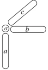
taking all indices together in one mode. A third-order rank-1 tensor can always be written as the outer product [9],

σ(_a◦_b◦_c) with components A_i1i2i3 = _{σ ai1bi2ci3}

with _σ ∈ R, whereas _a, _b, and _c are vectors of arbitrary lengths as depicted in Figure1. Similarly, any_d-way rank-1 tensor can be written as an outer product of_d vectors. Using the _k-mode multiplication, this outer product can also be written as σ×1a×2b×3c, whereσis now regarded as a 1×1×1 tensor. In order to facilitate the

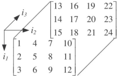
discussion of the TTr1 decomposition we will make use of a running example tensor

A ∈R3×4×2_{shown in Figure2.}

Fig. 1_{. The outer product of three vectors} a, b, c _{of arbitrary lengths forming a rank-1 outer}

product.

i1 i2 i3 1 4 7 10 2 5 8 11 3 6 9 12 13 16 19 22 14 17 20 23 15 18 21 24

Fig. 2_{.A running3}×₄×_{2tensor example.}

2. TTr1 decomposition.

2.1. TT decomposition. Our decomposition is directly inspired by the TT decomposition [15], which we will succinctly review here. The main idea of the TT decomposition is to re-express a tensorAas

(2.1) A_i1i2···id=G₁(_i1)G₂(_i2)· · · G_d(_id)_,

where for a fixed_ik eachG_k(_ik) is an_rk−1×_rk matrix, also called the TT core. Note that the subscript _k of a core G_k indicates the _kth core of the TT decomposition. The ranks _rk are called the TT ranks. Each core G_k is in fact a third-order tensor with indices_{αk−1, ik, αk} and dimensions_{rk−1, nk, rk}, respectively. SinceA_i1i2···idis a scalar we obviously have that_r0=_rd= 1 and for this reason_α0 and_αd are omitted. Consequently, we can write the elements ofAas

(2.2) A_i1i2···id= α1,···,αd−1

G1(i1, α1)G2(α1, i2, α2)· · · Gd(αd−1, id),

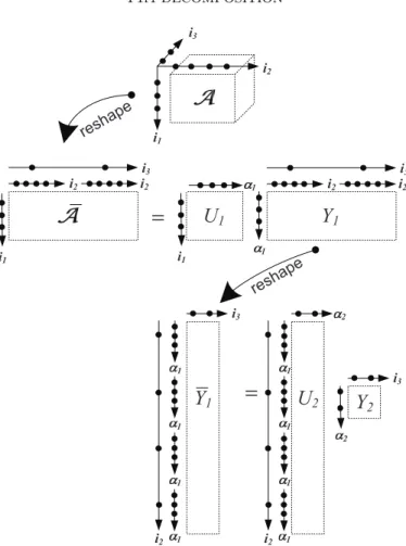
where we always need to sum over the auxiliary indices _{α1, . . . , αd−1}, and therefore (2.2) is equivalent to the matrix product form in (2.1). An approximation of A is achieved by truncating the_αk indices in (2.2) at values smaller than the TT ranks_rk. Computing the TT decomposition consists of doing_d−1 consecutive reshapings and SVD computations. For our running example A ∈ R3×4×2 in Figure 2, this means that the decomposition is computed in two steps. This process is visualized in Figure3, wherebyAwill eventually be converted into its TT format in Figure 4. Referring to Figure 3, the first reshaping of A into a matrix ¯A that needs to be considered is by grouping the indices_{i2, i3}together. This results in the 3×8 matrix

¯ A = ⎛ ⎝12 45 78 1011 1314 1617 2019 2223 3 6 9 12 15 18 21 24 ⎞ ⎠_. The “economical” SVD of the 3×8 matrix ¯Ais then

(2.3) A¯ = _U1S1V1T

with _U1 a 3×3 matrix and _V1 an 8×3 matrix. In fact, any dyadic decomposition can be used for this step in the TT algorithm, but the SVD is often chosen for its numerical stability. The first TT coreG₁is given by the 3×3 matrix_U1indexed by i1, α1. We now form the matrix _Y1 =_S1VT

1 and reshape it such that its rows are

i2 i2

=

U

Y

Y

=

U

Y

Fig. 3_{.Computation of the TT decomposition of}A_.

i

i

i

Fig. 4.TT decomposition ofA. Each set of orthogonal axes represents a coreGk of the TT.

indexed by _{α1, i2} and its columns by _i3. This results in a 12×2 matrix ¯_Y1 and its SVD

¯

Y1=_U2Y2 with_Y2=_S2VT

2 . The second TT coreG2is then given byU2, reshaped into a 3×4×2 tensor. The last TT coreG₃is then_Y2, which is a 2×2 matrix indexed by_α2and_i3.

We therefore have that

Ai1i2i3 =G1(i1)G2(i2)G3(i3)

withG₁(_i1) a 1×3 row vector,G₂(_i2) a 3×2 matrix, andG₃(_i3) a 2×1 column vector for fixed_{i1, i2}, and _i3, respectively (cf. Figure4). Observe how the auxiliary indices α1, α2serve as “links” connecting adjacent TT cores. For tensor orders_d≥3, besides the head and tail tensorsG₁(_i1)_,G_d(_id) which are in fact matrices, there will be (_d−2) third-order TT cores in between.

2.2. TTr1 decomposition. With the TT decomposition in place, we are now ready to introduce our TTr1 decomposition, which is easily understood from Figure5. The main idea of the TTr1 decomposition is to force the rank for each auxiliary index αk link to unity, which gives rise to a linear combination of rank-1 outer products. We go back to the first SVD (2.3) of the TT decomposition algorithm and realize that we can rewrite it as a sum of rank-1 terms

(2.4) A¯ =

3 i=1

σi×1ui×2vi,

where each vector_viis indexed by_{i2, i3}. The next step in the TT decomposition would be to reshape_Y1and compute its SVD. For the TTr1 decomposition we reshape each vi into an i2×i3 matrix ¯vi and compute its SVD. This allows us to write ¯v1 also as a sum of rank-1 terms

¯

v1 = _{σ11×1u11×2v11}+_{σ12×1u12×2v12.}

The same procedure can be done for_v2and_v3: they can also be written as a sum of two rank-1 terms. Combining these six rank-1 terms we can finally writeAas

A= ˜_{σ1×1u1×2u11×3v11}+ ˜_{σ2×1u1×2u12×3v12} (2.5)

+ ˜_{σ3×1u2×2u21×3v21}+ ˜_{σ4×1u2×2u22×3v22} + ˜_{σ5×1u3×2u31×3v31}+ ˜_{σ6×1u3×2u32×3v32}

with ˜_σ1 =_{σ1σ11, . . . ,σ6}˜ =_σ3σ32. Note the similarity of (2.5) with (2.4). The TTr1 decomposition has three main features that render it similar to the matrix SVD:

1. the scalars ˜_{σ1, . . . ,σ6}˜ are the weights of the outer products in the decompo-sition and can therefore be thought of as the singular values ofA,

2. the outer products affiliated with each singular value are tensors of unit Frobe-nius norm, since each product vector (or mode vector) is a unit vector, and 3. each outer product in the decomposition is orthogonal to all the others, which

we will prove in section3.

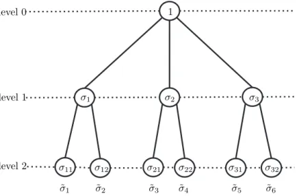
2.3. TTr1SVD algorithm. As was shown in the previous subsection, comput-ing the TTr1 decomposition requires recursively reshapcomput-ing the obtained_vvectors and computing their SVDs. This recursive procedure gives rise to the formation of a tree, where each SVD generates additional branches of the tree. The tree for the TTr1 decomposition of Ain (2.5) is shown in Figure6. As denoted in the figure, we will call a row in the tree a level. Level 0 corresponds to the SVD of ¯Aand generates the first level of singular values. This is graphically represented by the node at level 0 branching off into three additional nodes at level 1. The reshaping and SVD of the different _v vectors at level 1 then generates level 2 and so forth. Observe how the

i1 u1 V1

+

=

+

+

=

+

=

+

=

Fig. 5.Computation of the TTr1decomposition ofA.

σ1 σ2 σ11 σ12 σ21 σ22 level 1 level 2 level 0 σ3 σ31 σ32 1 ˜ σ1 _σ2˜ _σ3˜ _σ4˜ _σ5˜ ˜_σ6

Fig. 6_{. Tree representation of TTr1decomposition, where}σ_{˜i is the product of all nodes down}

a branch.

total number of subscript indices of the singular values are equal to the level at which these singular values occur. For example,_σ2 occurs at level 1 and_σ21occurs at level 2. The number of levels for the TTr1 decomposition of an arbitrary _d-way tensor is d−1. The final singular values ˜_σi’s are the product of all_σ’s along a branch.

The total number of terms in the decomposition is the total number of leaves. This number is easily determined. Indeed, each node at level_kof the tree branches off into rk min nk+1, d i=k+2 ni (k= 0, . . . , d−2)

nodes. Hence, the total number of leaves or terms _N in the TTr1 decomposition is given by N = d−2 k=0 rk.

The algorithm to compute the TTr1 decomposition is presented in pseudocode in Algorithm 1. First the tensor A is reshaped into an _n1×d_i=2ni matrix and its SVD is computed. The computational complexity for this first step is approximately 14_n2₁d_i=2ni+ 8_n3₁ flops. Observe that the computation of the TT or Tucker de-composition has a computational complexity of the same order of magnitude. Then for all remaining nodes in the tree, except for the leaves, the resulting_vi vectors are reshaped into a matrix and their SVDs are also computed. The_{U, S, V} matrices for each of these SVDs are stored. Note that for levels 0 up to _d−2 the _v vectors do not need to be stored. From the tree it is also easy to determine the total number of SVDs required to do the full TTr1 decomposition. This is simply the total number of nodes in the tree from level 0 up to_d−2 and equals

1 + d−3 i=0 i k=0 rk.

Assuming that _rk =_nk for all _k, then the total number of SVDs required for com-puting the TTr1 decomposition of a cubical tensor is

1 +_n+_n2+· · ·+_nd−2 = 1−n d−1 1−_n .

This exponential dependence on the order of the tensor and the computational com-plexity of _O(_n2₁ d_i=2ni) for the first SVD are the two major limiting factors to compute the TTr1 decomposition. Note, however, that the tree structure is perfectly suited to do all SVD computations that generate the next level in parallel, and in that case the runtime is linearly proportional to the number of levels. However, such an implementation requires an exponential growing number of computational units.

Input: arbitrary tensorA

Output: _{U, S, V} matrices of each SVD

¯

A ←reshapeAinto an_n1×d_i=2ni matrix U1, S1, V1←SVD( ¯A)

forall remaining nodes in the tree except the leavesdo ¯ vi←reshapevi Uk, Sk, Vk←SVD(¯vi) add_{Uk, Sk, Vk} to _{U, S, V} end for Algorithm 1. _TTr1SVD.

3. Properties. We now discuss many attractive properties of the TTr1 decom-position. Most of these properties are also shared with the matrix SVD and it is in this sense that the TTr1SVD is a natural generalization of the SVD for tensors.

3.1. Uniqueness. A first attractive feature of the TTr1 decomposition is that it is uniquely determined for a fixed order of indices. This means that for any given arbitrary tensor A its TTr1 decomposition will always be the same. Indeed, Algo-rithm1 consists of a sequence of SVD computations so the uniqueness of the TTr1 decomposition follows trivially from the fact that each of the SVDs in Algorithm 1

is unique up to sign. Although the singular values and vectors of a matrix_A and its transpose_AT are the same, this is not the case for the TTr1SVD. Indeed, applying a permutation of the indices_π(_{i1, . . . , in}) will generally result in a different TTr1SVD, which we illustrate in Example 1 in section4.1. Once the indices are fixed, however, the TTr1SVD algorithm will always return the same decomposition, which is not the case for conventional iterative optimization-based methods.

3.2. Orthogonality of outer products. Any two rank-1 terms ˜_σiT_i and ˜_σjT_j of the TTr1 decomposition are orthogonal with respect to one another, which means thatT_i,T_j= 0. We will use our running example to show why this is so. Let us take two terms of (2.5), for example,T₁= 1_{×1u1×2u11×3v11} and T₂ = 1_{×1u1×2u12×3v12}. Another way of writing T_1,T₂is

T1,T2 = (v11⊗u11⊗u1)T(v12⊗u12⊗u1),

where ⊗ denotes the Kronecker product. These Kronecker products generate the vectorization of each of the rank-1 tensorsT_1,T₂, which allows us to easily write their inner product as an inner product between two mode vectors. Applying properties of the Kronecker product we can now write

(_v11⊗_u11⊗_u1)T(_v12⊗_u12⊗_u1) =_v11T ⊗_uT₁₁⊗_uT₁(_v12⊗_u12⊗_u1)_, =_vT_11v12⊗_u11T _u12⊗_uT_1u1,

where it is clear that the right-hand side vanishes due to the orthogonality_vT_11v12= uT11u12 = 0. This property generalizes to any tensorA. Indeed, if any two rank-1 terms do not originate from the same node at level 1, then their respective _{ui, uj} vectors are orthogonal and ensure that their inner product vanishes. If the two rank-1 terms do originate from the same node at level rank-1 but from different nodes at level 2, then their_{uij, uik} vectors are orthogonal and again the inner product will vanish. This reasoning extends up to level _d−1. If any two terms have their first separate nodes at level_k∈[1_{, d}−1], then their corresponding_uvectors at level_kwill also be orthogonal. The tree structure, together with the orthogonality of all_uvectors that share a same parent node, hence guarantees that any two rank-1 outer factors in the TTr1 decomposition are orthogonal. The TTr1 decomposition is hence an orthogonal decomposition as defined in [8].

3.3. Upper bound on the orthogonal tensor rank. The (CP-)rank of an ar-bitrary_d-way tensorAis usually defined similarly to the matrix case as the minimum number of rank-1 terms thatAdecomposes into.

Definition 3.1. The rank of an arbitrary d-way tensor A, denoted rank(A), is the minimum number of rank-1 _{tensors that yields} A_{in a linear combination.}

In [8, 12] the orthogonal rank, rank_⊥(A), is defined as the minimal number of terms in an orthogonal rank-1 decomposition. Apparently,

rank(A)≤rank_⊥(A)_,

where strict inequality is possible for tensors of orders_{d >}2. The TTr1 decomposition allows a straightforward determination of an upper bound on rank_⊥(A). Indeed, this is simply the total number of leaves in the tree and is therefore

(3.1) rank_⊥(A) ≤ _N =

d−2 k=0

rk. Applying (3.1) to our running exampleA ∈R3×4×2 we obtain

rank_⊥(A) ≤ min(3_,8)·min(4_,2) = 3·2 = 6_. For a cubical tensor with_n1=· · ·=_nd=_n, (3.1) then tells us that

rank_⊥(A) ≤ d−2 k=0 min(_{n, n}d−1) = d−2 k=0 n=_nd−1_.

The dependency of the TTr1SVD on the ordering of the indices implies that a per-mutation of the indices can lead to different upper bounds on the orthogonal rank. Indeed, if we permute the indices ofAto{_{i2, i3, i1}}we get

rank_⊥(A) ≤ min(4_,6)·min(2_,3) = 4·2 = 8_.

Consequently, there exists the notion of a minimum upper bound on the orthogonal rank of a tensor, obtained from computing the rank upper bounds through all per-mutations of indices. Whether the TTr1SVD algorithm is able to derive a minimal orthogonal decomposition needs further investigation. Furthermore, we will demon-strate by an example in section 4 that the orthogonality as it occurs in the TTr1 decomposition is not enough to make the problem of computing a low-rank approxi-mation of an arbitrary tensor well-posed. This agrees with [21], in which a necessary condition of pairwise orthogonality of all rank-1 terms in at least two modes is proved. 3.4. Quantifying the approximation error. As soon as the number of levels is large it becomes very cumbersome to write all the different subscript indices of the u and _v vectors in the TTr1 decomposition. We therefore introduce a shorter and more convenient notation. Herein,_ukidenotes the_uvector at level_kthat contributes to the_ith rank-1 term. Similarly,_vi denotes the_v vector that contributes to the_ith rank-1 term. The TTr1SVD algorithm decomposes an arbitrary tensorAinto a linear combination of_N orthogonal rank-1 terms

(3.2) A = N i=1 ˜ σi×1u1i×2u2i×3. . .×d−1ud−1i×dvi with ||1_{×1u1i×2u2i×3. . .×d−1ud−1i×dvi}||_F = 1 and _N = d−2 k=0 rk.

Suppose that we have ordered and relabeled the terms such that ˜_σ1≥_σ2˜ ≥ · · · ≥˜_σN. An_R-term approximation is then computed by truncating (3.2) to the first_Rterms

˜ A = R i=1 ˜ σi×1u1i×2u2i×3. . .×d−1ud−1i×dvi.

The following lemma tells us exactly what the error is when breaking off the summa-tion at_Rterms.

Lemma 3.2. Let A˜be the summation of the firstR terms in (3.2). Then

||A −_A||˜ F =

˜

σR2+1+· · ·+ ˜σ2N.

Proof. Using the fact that||1_{×1u1i×2u2i×3. . .×d−1ud−1i×dvi}||_F = 1 we can write

||A −_A||˜ F = n i=R+1 ˜ σi×1u1i×2u2i×3. . .×d−1ud−1i×dvi F = ˜ σ2R+1+· · ·+ ˜σN2. Lemma 3.2can also be used to determine the lowest number of terms _R with a guaranteed accuracy. Indeed, once a toleranceis chosen such that it is required that

||A −_A||˜ F ≤ ,

the minimal number of terms_Rin the TTr1 decomposition of ˜Ais easily determined by the requirement that

˜ σ2_R+1+· · ·+ ˜_σN2 ≤such that ˜ σ_R2 +· · ·+ ˜_σN2 _{> .}

It is tempting to choose_Rsuch that ˜_{σR> >}˜_σR+1. However, when the approxi-rank gap, defined as ˜_σR/σ˜_R+1 [13, p. 920], is not large enough, then there is a possibility that√_σ˜2_R+1+· · ·+ ˜_σN2 ≥due to the contributions of the smaller singular values. A large approxi-rank gap implies that the number of terms in the approximation ˜Ais relatively insensitive to the given tolerance. In Example 6 in section4.6a tensor is presented for which this is not the case.

3.5. Reducing the number of SVDs. Suppose that an approximation ˜Aof

Ais desired such that||A −A||˜ _F ≤ . Computing the full TTr1 decomposition and applying Lemma3.2solves this problem. It is, however, possible to reduce the total number of required SVDs by taking into account that the final singular values ˜_σi’s are the product of the singular values along each branch of the TTr1-tree. An important observation is that all singular values_σij···mat levels 2 up to_d−1 satisfy_σij···m≤1. This is easily seen from the fact that they are computed from a reshaped unit vector vij···n at their parent node. Indeed, since||vij···n||2= 1 it follows that||¯vij···n||F = 1. This allows us to make an educated guess about the impact of the singular values at level _l on the final rank-1 terms. Suppose we have a singular value_σk at level _l, preceded by a product _σk0 of parent singular values. An upper bound on the size of the final ˜_σ’s that are descendants from_σk can be derived by assuming that_σk is unchanged throughout each branch. Since one node at level_lresults ind_i=−2_{l ri}rank-1 terms, this then implies that there ared_i=−2_{l ri} rank-1 terms with ˜_σ=_σk0σd_k−l−1, so

˜ σ12+· · ·+ ˜σ2N ≤σ˜21+· · ·+ ˜σ2r+ d−2 i=l ri(σk0σd_k−l−1)2. If now (3.3) _e2_k d−2 i=l ri(σk0σ_kd−l−1)2≤2

is satisfied, then removing_σk at level_l produces an approximation ˜Athat is guaran-teed to satisfy the approximation error bound. Removing _σk at level _l implies that not a full but a reduced TTr1 decomposition is computed. Indeed, the total number of computed rank-1 terms is effectively lowered byd_i=−2_{l ri}terms, decreasing the total number of required SVDs in the TTr1SVD algorithm. This condition on_σk is easily extended to_msingular values at level_l as

(3.4)

m j=1

e2j≤2,

where we compute an_ej term for each of the_msingular values at level_l. Checking whether (3.4) holds for _{m σ}’s at level _l can be easily implemented in Algorithm 1. As shown in section4, a rather gradual decrease of_σk is seen in practice as the level increases. This implies that it might still be possible to find an ˜Aof lower rank that satisfies the approximation error bound from the rank-1 terms of a reduced TTr1 decomposition. Lemma3.2can also be used to find the desired ˜Ain this case.

3.6. Orthogonal complement tensors. We can consider the vectorization of

Aas a vector living in an (_n1· · ·_nd)-dimensional vector space. Naturally, there must be an (_n1· · ·_nd−1)-dimensional vector space opspan(A)⊥ of tensors that are or-thogonal to A. Note that each basis vector of opspan(A)⊥ is required to be the vectorization of an outer product of vectors. The TTr1 decomposition allows us to easily find an orthogonal basis for opspan(A)⊥. We will illustrate how this comes about using tensorAfrom Figure2and notions in (2.5). Recall from section2.2that the first step in the TTr1SVD algorithm was the economical SVD of the 3×8 matrix

¯

A=_{U SV}T_{. Each of the v}

i vectors was then reshaped into a 4×2 matrix ¯vi. Now consider a full SVD of each of these ¯_vi matrices,

(3.5) ¯_vi = _{ui1 ui2 ui3 ui4} ⎛ ⎜ ⎜ ⎝ σi1 0 0 _σi2 0 0 0 0 ⎞ ⎟ ⎟ ⎠ viT1 viT2 ,

which is a sum of eight orthogonal rank-1 outer products with only two nonzero_σ’s. There are hence six additional outer product terms_ui◦_uij◦_vij with a zero singular value, orthogonal to the outer product terms of the economical TTr1 decomposition (2.5). It is easily seen that the rank-1 terms obtained from the zero entries of the_S matrix in (3.5) are orthogonal to A and are therefore basis vectors of opspan(A)⊥. Table1lists all eight orthogonal rank-1 outer product terms that are obtained for the u1branch in the TTr1-tree. Each rank-1 term can be read off from Table1by starting from the top row and going down along a particular branch of the TTr1-tree. For example, the fourth rank-1 term is given by ˜_σ2u1◦_u12◦_v12 and the seventh rank-1 term by 0_u1◦_u14◦_v11. We call such a table that exhibits the TTr1-tree structure and allows us to reconstruct all rank-1 terms an outer product column table. The extra orthogonal terms for the_{u2, u3} branches are completely analogous to the_u1 branch. Note that the economical TTr1 decomposition described in section2.2computes only the ˜_σ1u1◦_u11◦_v11 and ˜_σ2u1◦_u12◦_v12terms.

The full TTr1 decomposition therefore consists of 8×3 = 24 orthogonal terms and can be written in vectorized form as

Table 1

All eight orthogonal rank-1outer products in theu1 branch of the TTr1-tree.

u1

u11 u12 u13 u14

v11 v12 v11 v12 v11 v12 v11 v12

˜

σ1 0 0 σ˜2 0 0 0 0

vec(A) = vec(T₁) · · · vec(T₆) vec(T₇) · · ·vec(T₂₄) ⎛ ⎜ ⎜ ⎜ ⎜ ⎜ ⎜ ⎜ ⎜ ⎝ ˜ σ1 .. . ˜ σ6 0 .. . 0 ⎞ ⎟ ⎟ ⎟ ⎟ ⎟ ⎟ ⎟ ⎟ ⎠ ,

where vec(T₁)_{, . . . ,}vec(T₆) are the orthogonal terms computed in section 2.2 and vec(T₇)_{, . . . ,}vec(T₂₄) are the orthogonal terms that partly span opspan(A)⊥. Note that we have found only 18 basis vectors for opspan(A)⊥. The remaining 5 basis vectors are to be found as the following linear combinations of vec(T₁)_{, . . . ,}vec(T₆),

vec(T₁) · · · vec(T₆)_S⊥_,

where_S⊥is the 6×5 matrix orthogonal to˜_σ1 · · · _σ6˜ . The property that for every tensor B ∈opspan(A)⊥ we have that A_,B = 0 allows us to interpret opspan(A)⊥ as the orthogonal complement of vec(A).

3.7. Constructive proof of the maximal CP-rank of a 2×2×2 tensor. As an application of the outer product column table, we show how it leads to an elegant proof of the maximal CP-rank of a real 2×2×2 tensor overR. It is known that the maximum rank of a real 2×2×2 tensor overR is 3 (i.e., any such tensor can be expressed as the sum of at most three real outer products [9]), for which rather complicated proofs were given in [11,19]. Incidentally, we show that the TTr1 decomposition allows us to formulate a remarkably simpler proof. As in section3.6, we first consider all orthogonal outer products that spanR2×2×2in the outer product table, Table2.

Table 2

Outer product table for a general2×2×2tensor.

u1 u2

u11 u12 u21 u22

v11 v12 v11 v12 v21 v22 v21 v22

˜

σ1 0 0 σ˜2 σ˜3 0 0 ˜σ4

The columns in Table 2 with nonzero singular values are the “active” columns in the TTr1 decomposition of a random real tensor A ∈ R2×2×2. The “inactive” (orthogonal) columns carry zero weights but are crucial for proving the maximum rank-3 property ofA.

We first enumerate two important yet straightforward properties for the columns in Table2, ignoring the bottom row for the time being. First, scaling a column can be regarded as multiplying a scalar onto the whole outer product or absorbing it into

any one of the mode vectors. Taking the first column and a scalar_α∈Rfor instance, this means that

α(_u1◦_u11◦_v11) = (_αu1)◦_u11◦_v11=_u1◦(_αu11)◦_v11=_u1◦_u11◦(_αv11)_. In other words, the scalar is “mobile” across the various modes. The second property is that any two columns differing in only one mode can be added to form a new rank-1 outer product [8]. We list two examples showing the rank-1 outer products resulting from the linear combinations of columns 1 and 3, and columns 3 and 4, respectively,

α(_u1◦_u11◦_v11) +_β(_u1◦_u12◦_v11) =_u1◦(_αu11+_βu12)◦_v11, α(_u1◦_u12◦_v11) +_β(_u1◦_u12◦_v12) =_u1◦_u12◦(_αv11+_βv12)_.

Now to prove the maximum rank-3 property ofA then is to show that the four active columns of the outer product column in Table2 can always be “merged” into three. To begin, it is readily seen that if we add any nonzero multiple of column 3 to column 1, and then subtract the same multiple of column 3 from column 4, the overall tensor by summing all columns in Table2remains unchanged. Our final goal is to merge columns 1 and 5 into one outer product by making two of their modes the same (up to a scalar factor). This is done by appropriately adding column 3 to column 1 such that the second mode vectors of columns 1 and 5 align, while adding column 6 to column 5 such that the third mode vectors of columns 1 and 5 align. Of course, subtractions of column 3 from column 4, and column 6 from column 8, respectively, are necessary to offset the addition. This intermediate step is summarized in Table3, where the four intermediate columns are now shown individually with the ˜

σi’s absorbed into the mode vectors.

Table 3

The four intermediate outer products that can be merged into three outer products.

u1 u1 u2 u2 ˜ σ1u11 ˜σ4u22 +αu12 u11 u21 −γu21 (=βu21) −αv11 ˜σ3v21 v11 +˜σ2v12 +γv22 v22 (=δv11)

The two linear equations that need to be solved in this process are −u12 u21 α β = ˜_σ1u11 and −_{v22 v11} γ δ = ˜_σ3v21.

It is not hard to see that columns 1 and 3 of Table 3 can now be merged into one outer product,

(_βu1+_δu2)◦_u21◦_v11,

due to two of their mode vectors now being parallel. Hence an overall rank-3 repre-sentation for the original tensorAis obtained from its TTr1 decomposition.

Obviously, this rank-3 representation is not unique since alternatively we can first align the third mode of columns 1 and 5, followed by their second mode. Fur-thermore, instead of columns 1 and 3, we can also merge columns 2 and 4, etc.

Details are omitted as they are all based on the same idea of merging columns. An-other big advantage of our rank-3 construction is that the relative numerical error

||A −_A||˜

F/||A||F <10−15, whereas the CP rank-3 decomposition has a median error of≈10−6 over a 100 trials of arbitrary 2×2×2 tensors.

3.8. Perturbations of singular values. When an_m×_nmatrix_Ais additively perturbed by a matrix _E to form ˆ_A=_A+_E, then Weyl’s theorem [18] bounds the absolute perturbations of the corresponding singular values by

|σi−σˆi| ≤ ||E||2,

where the ˆ_σi’s are the singular values of ˆ_A. It is possible to extend Weyl’s theorem to the TTr1 decomposition of the perturbed tensor ˆA=A+E. Suppose we want to determine an upper bound for the perturbation of one of the singular values ˜_σ. We first introduce the simpler notation

˜

σ=_σ1σ2 · · ·_σd−2,

where_σk(_k= 1_{, . . . , d}−2) denotes the singular value at level _kin the branch of the TTr1-tree corresponding with ˜_σ. Applying Weyl’s theorem to the first factor gives

|σ1−ˆ_σ1| ≤ ||E||¯ _2, which we can rewrite into

(3.6) |_σ1ˆ | ≤ |_σ1|+||E||¯ _2.

Each of the remaining factors_{σ2, . . . , σd−2} are the singular values of a reshaped right singular vector_{v1, . . . , vd−3}. Again, application of Weyl’s theorem allows us to write

|ˆ_σk| ≤ |_σk|+||Δ¯_vk−1||₂ (_k= 2_{, . . . , d}−2)_,

≤ |σk|+||Δ¯vk−1||F =|σk|+||Δvk−1||2 (k= 2, . . . , d−2). (3.7)

An upper bound for the ||Δ¯_vk−1||₂ term is difficult to derive. Fortunately, it is pos-sible to replace the||Δ¯_vk−1||₂ term by||Δ¯_vk−1||_F =||Δ_vk−1||₂, for which first-order approximations exist [14]. Multiplying (3.6) with (3.7) over all_kwe obtain

|_σ1ˆ | · · · |_σˆ_d−2| ≤(|_σ1|+||E||¯ ₂)· · ·(|_σk|+||Δ_vk−1||₂)_, which can be simplified by ignoring higher-order terms to

(3.8) |_σ1ˆ | · · · |_σˆ_d−2| ≤ |_σ1| · · · |_σd−2|+|_σ2| · · · |_σd−2| ||E||¯ ₂+ d−2 k=2 ⎛ ⎝ i=k |σi| ⎞ ⎠_||Δ_vk−1||_2. The maximal value for_{σ2, . . . , σd−2}is 1 and hence (3.8) can be written as

|_σ1ˆ | · · · |_σˆ_d−2| ≤ |_σ1| · · · |_σd−2|+||E||¯ ₂+_{σ1 d−3}

k=1

||Δ_vk||_{2 .} Hence we arrive at the expression

(3.9) |_σ˜−_σˆ˜| ≤ ||E||¯ ₂+_{σ1 d−3}

k=1

||Δ_vk||_{2 ,}

which generalizes Weyl’s theorem to the TTr1 decomposition by the addition of a cor-rection term_σ1(d_k−3₌₁||Δ_vk||₂). This correction term depends on the largest singular value of the first level and the perturbations on the right singular vectors for levels 1 up to_d−3.

3.9. Conversion to the Tucker decomposition. It is possible to convert the sum of orthogonal rank-1 terms obtained from a (truncated) TTr1 decomposition into the Tucker decomposition,

A = S_×1U1×2U2· · ·_×dUd, whereS ∈Rr1×r2×···×rd_{is called a core tensor andU}

k∈Rnk×rk are orthogonal factor matrices. In this way it becomes relatively easy to compute an approximation of a tensor with a known approximation error in the Tucker format with orthogonal factor matrices. This conversion is easily achieved using simple matrix operations. To avoid notational clumsiness, we illustrate the conversion from the TTr1 representation into the Tucker form through the specific TTr1 decomposition in (2.5). Suppose only alternate terms in the equation are significant and we therefore keep only the three terms associated with _σ1σ11, _σ2σ21, and _σ3σ31. Then, the mode vectors of these outer products are collected and subjected to economic QR factorization. We note that _U1 = [_{u1 u2 u3}]∈R3×3 is already orthogonal and does not need to go through a QR factorization, while

u11 u21 u31=_{q21 q22 q23} U2 ⎡ ⎣10 α12_α22 α13_α23 0 0 _α33 ⎤ ⎦_, v11 v21 v31=_{q31 q32} U3 1 _{β12 β13} 0 _{β22 β23} . Consequently, the truncated TTr1SVD of (2.5) reads

A ≈σ1σ11(_u1◦_u11◦_v11) +_σ2σ21(_u2◦_u21◦_v21) +_σ3σ31(_u3◦_u31◦_v31) =_σ1σ11(_u1◦_q21◦_q31) +_σ2σ21(_u2◦(_α12q21+_α22q22)◦(_β12q31+_β22q32))

+_σ3σ31(_u3◦(_α13q21+_α23q22+_α33q23)◦(_β13q31+_β23q32)) =S_{×1U1×2U2×3U3,}

(3.10)

where the core tensorS ∈R3×3×2 is filled with coefficients found through expanding the outer products and collecting terms in (3.10). Observe that the dimensions of the core tensorS are completely determined by the ranks of the orthogonal factor matri-ces. From practical examples we observe that the Tucker core obtained in this way is more sparse compared to the Tucker core computed from the ALS algorithm [2, 3]. If we take, for example, a random tensor in∈R4×3×15, then its TTr1 decomposition consists of 12 terms. The ranks of the orthogonal factor matrices_{U1, U2, U3} are then 4_,3_,12, respectively. Consequently, we have that S ∈ R4×3×12 with 3 + 3·9 = 30 nonzero entries. In contrast, computing the Tucker decomposition using the ALS method results in a maximally dense core tensor of 144 nonzero entries.

4. Numerical examples. In this section, we demonstrate some of the proper-ties of the TTr1 decomposition and compare it with the ALS-CP and Tucker decom-positions by means of numerical examples. All experiments are done in MATLAB on a desktop computer. A MATLAB/Octave implementation of the TTr1SVD algorithm can be freely downloaded and modified fromhttps://github.com/kbatseli/TTr1SVD. The ALS-CP and Tucker decompositions are computed by the ALS optimization tool provided in the MATLAB Tensor Toolbox [2, 3]. All ALS procedures are fed by random initial guesses; therefore their errors are defined as the average error over multiple executions.

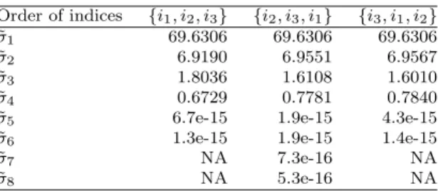
Table 4 ˜ σ’s of TTr1decomposition forA. Order of indices {i1, i2, i3} {i2, i3, i1} {i3, i1, i2} ˜ σ1 69.6306 69.6306 69.6306 ˜ σ2 6.9190 6.9551 6.9567 ˜ σ3 1.8036 1.6108 1.6010 ˜ σ4 0.6729 0.7781 0.7840 ˜

σ5 6.7e-15 1.9e-15 4.3e-15

˜

σ6 1.3e-15 1.9e-15 1.4e-15

˜

σ7 NA 7.3e-16 NA

˜

σ8 NA 5.3e-16 NA

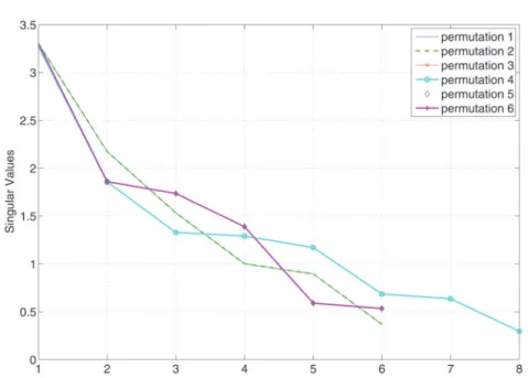
4.1. Example 1: Singular values and permutation of indices. We start with tensor Ain Figure2. Since it is discussed in section3.3that TTr1 decomposi-tion depends on the ordering of the indices, we demonstrate the TTr1 decomposidecomposi-tion with different permutations of the indices. For a three-way tensor, the order of in-dices can be {_{i1, i2, i3}}, {_{i1, i3, i2}}, {_{i2, i1, i3}}, {_{i2, i3, i1}}, {_{i3, i1, i2}}, or {_{i3, i2, i1}}. Since the order of the last two indices will not affect the_σ’s in TTr1 decomposition, we only list the _σ’s under the permutations{_{i1, i2, i3}}, {_{i2, i3, i1}}, and {_{i3, i1, i2}} in Table 4, in descending order. As a result, although permutations of indices may give different upper bounds on the rank, TTr1 decomposition still outputs the same rank(A) = 4 in all permutations. The largest (dominant) singular value (69.6306) differs only slightly with respect to the permutations, which is also the general ob-servation. Note that the singular values are quite similar over all permutations for this example. It can also be seen that some singular values are numerically zero. The same threshold commonly used to determine the numerical rank of a matrix using the SVD can also be used for the TTr1 decomposition. An interesting consequence of the rank-deficiency of Ais that we can interpret the rank-1 terms corresponding with the very small numerical singular values as being related to opspan(A)⊥. For the {_{i1, i2, i3}}_,{_{i3, i1, i2}} permutations there are two extra orthogonal complement tensors, while for the{_{i2, i3, i1}} there are four extra orthogonal complement tensors. Figure7shows the similar singular value curves for all six permutations of a random 3×4×2 tensor, where it can also be seen that there are basically three distinct permu-tations and that the largest singular values differ only slightly over all permupermu-tations. 4.2. Example 2: Comparison with ALS-CP and Tucker decomposition. Next, ALS-CP is applied onA. To begin, we compute the best rank-1 approximation of A. ALS-CP gives the same weight 69.6306 as the TTr1 decomposition, implying that both decompositions result in the same approximation in terms of the Frobenius norm. The errors betweenAand its approximations ˜A, computed using the ALS-CP and TTr1SVD method, are listed in Table5for increasing rank.

Table 5 confirms that the rank_⊥(A) = rank(A) = 4. It also indicates that as an optimization approach, ALS-CP itself cannot determine the rank, only the best rank-_R approximation for a specific _R. Furthermore, it should be noticed that the TTr1 decomposition can always give an_R-rank-1-term approximation with orthonor-mal outer products, while ALS-CP cannot ensure this property. Finally, a Tucker decomposition with a core size (2_,2_,2) is applied on A. The resulting dense core tensorS ∈R2×2×2 is given by Si1i21= 69_.6306 −0_.0181 −0_.0701 −0_.7840 , Si1i22= −0_.0113 −6_.9190 −1_.6108 −0_.7010 .

Fig. 7_{.Singular value curves for each of the six permutations of a random3}×₄×_2tensor.

The rank-1 outer factors obtained from the Tucker decomposition are also orthonor-mal. However, compared to the TTr1 decomposition, the Tucker format needs twice the number of rank-1 terms than TTr1.

Table 5

Errors||A −A||F˜ of ALS-CP and TTr1SVD for increasing rankR.

Rank 1 2 3 4 5

TTr1SVD 7.2 1.9 0.7 6.8e-15 1.3e-15 ALS-CP 7.2 0.8 3.6e-2 1.4e-10 4.7e-11

4.3. Example 3: Rank behavior under largest rank-1 term subtraction. In this example we investigate the behavior of the singular value curves and the rank when the largest rank-1 term obtained from the TTr1 decomposition is consecutively subtracted. This means that we start with A from Figure 2, compute its largest orthogonal rank-1 term T₁ from the TTr1 decomposition, and subtract it to obtain

A−T1, after which the procedure is repeated. Figure8shows the singular value curves from the TTr1 decompositions obtained for each of the iterations, where it is easily seen that each curve gets shifted to the left with each iteration. In other words, the largest singular value in the next iteration is the second largest singular value of the previous iteration, etc. It is also clear that subtracting the largest orthogonal rank-1 term does not necessarily decrease the rank as also described in [17]. Indeed, using a numerical threshold of max(4_,8)·1_.11×10−16·_σ1 = 1_.13×10−13 on the singular values obtained in the first iteration will still return a numerical orthogonal rank of 4. In addition, the rank of the obtained tensors in each iteration was also determined from the CP-decomposition. From Table 5, a numerical threshold of 10−10 was set to the absolute error ||A −A||˜ _F to determine the CP-rank. In Table 6, both the CP-rank and the orthogonal rank from the TTr1 decomposition are compared. It can be seen that the rank determined from ALS-CP increases while the orthogonal

Fig. 8.Singular value curves for consecutive subtractions of the largest rank-1term. Table 6

Ranks determined by ALS-CP and TTr1decomposition for consecutive subtraction of the largest rank-1term.

Iteration 0 1 2 3 4 5

CP-rank 4 4 4 5 3 2

TTr1 rank 4 4 4 4 3 2

rank monotonically decreases. In this sense, the orthogonal rank appears to be more robust under the largest rank-1 term subtraction.

4.4. Example 4: Perturbation of the singular values. In this example we illustrate the robustness of the computed singular values of our running example tensorAwhen it is subjected to additive perturbations. We construct a perturbation tensorE ∈R3×4×2where each entry is drawn from a zero mean Gaussian distribution with variance 10−6. We then compute the following two norms ofE and ¯E:

||E||F = 5.48×10−6 and ||E||¯ 2 = 4.13×10−6,

where ¯E isE reshaped into a 3×8 matrix. Comparing the perturbed singular values ¯

˜

σ1, . . . ,_σ6¯˜ ofA+E with the singular values ˜_{σ1, . . . ,σ6}˜ then shows that (4.1)

(¯_σ1˜ −_σ1˜ )2+· · ·+ (¯_σ6˜ −_σ6˜ )2= 3_.78×10−6_<||E||_F and

(4.2) |_σ¯˜_i−˜_σi| ≤ ||E||¯ ₂ (_i= 1_{, . . . ,}6)_.

These two inequalities (4.1) and (4.2) are very reminiscent of Mirsky’s and Weyl’s theorems [18], respectively, for the perturbation of singular values for matrices.

4.5. Example 5: Gradual decrease of intermediate singular value products. In the discussion on reducing the total number of required SVDs it was shown that the product of the singular values along a branch becomes smaller and smaller for every additional level. In this example we demonstrate this gradual de-crease for a random 2×2×2×2×2 tensor where each entry is drawn from a zero mean Gaussian distribution with variance 1. The TTr1 decomposition always has 16 rank-1 terms. Figure9shows the intermediate singular value products_σiσij· · ·_σij···m as a function of the level for ˜_σ1,˜_σ8,σ13,˜ _σ16˜ . The figure shows that the intermediate singular value products indeed decrease as the level increases. The TTr1-tree for this tensor is a binary tree. Each SVD of a_vvector therefore produces 2 singular values. It is consistently observed that of the two singular values of ¯_v, one is very close to unity, with values around 0_.8 or 0_.9. The other singular value typically has values around 0_.5. Branches of the tree that mostly choose the singular value close to unity therefore exhibit a very slow decrease, while branches that predominantly choose the smaller singular value decrease faster. This is seen in Figure9 as a bigger descent of the intermediate products of ˜_σ8,σ16˜ compared to ˜_σ1,σ13˜ .

Fig. 9_{.Gradual decrease of intermediate singular value products as a function of the level.}

4.6. Example 6: Exponential decaying singular values. In this example we illustrate the computation of an approximation ˜A using Lemma 3.2 when the singular values ˜_σdecay exponentially. Consider the tensorA ∈R5×5×5 with

Ai1i2i3 =

1 i1+_i2+_i3,

which has very smoothly decaying singular values, as shown in Figure 10. There are a total number of 25 rank-1 terms in the TTr1 decomposition. Suppose we are interested in obtaining an approximation ˜Asuch that|A−A||˜ _F ≤10−6. Sorting the

rank-1 terms by descending singular values and using Lemma3.2, the approximation would then consist of 17 terms since

˜

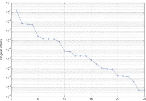
σ16= 3_.18×10−6≥_σ17˜ = 1_.18×10−6≥1_.00×10−6≥_σ18˜ = 9_.00×10−7_. The approxi-rank gap ˜_σ17/σ18˜ = 1_.31, which indicates that there is no clear “gap” between ˜_σ17 and ˜_σ18. In contrast, the tensor in Example 1 (section 4.1) has an approxi-rank gap of ˜_σ4/˜_σ5 ≈ 1014. Also note that it is not possible to reduce the number of SVDs during execution of the TTr1SVD algorithm since none of the first five computed singular values_{σ1, . . . , σ5} satisfy condition (3.3), with _σk0= 1. Next, the approximations obtained from the TTr1 decomposition and CP decomposition of this tensor are compared for increasing rank. The CP decomposition was computed over 10 trials with different initial guesses using the CP-ALS method. The absolute errors in terms of the rank are listed in Table7. For the CP decomposition case the mean absolute error over the 10 trials is reported. From Table 7 it is seen that the errors are almost identical up to the first 24 terms. Since the TTr1 decomposition consists of 25 terms, the error drops at that term to the order of the machine precision, while the ALS-CP method fails to produce any significant improvement in the error. Even when a CP decomposition of 100 rank-1 terms are computed, the average absolute error is around 10−12.

Fig. 10_{. Singular value decay of the function-generated tensor}Ai

1i2i3 = 1/(i1+i2+i3).

Table 7

Errors||A −A||F˜ of ALS-CP and TTr1SVD for increasing rankR.

Rank 1 5 10 15 20 25

TTr1SVD 9.5e−2 2.6e−3 7.6e−5 3.6e−6 2.2e−7 9.9e−16 ALS-CP 9.5e−2 1.6e−3 3.6e−5 4.5e−6 1.2e−7 1.6e−7