Multi-objective particle swarm optimization algorithm for multi-step electric load forecasting

(1)

Article

Multi-Objective Particle Swarm Optimization

Algorithm for Multi-Step Electric Load Forecasting

Yi Yang1, Zhihao Shang2,*, Yao Chen1and Yanhua Chen3

1 _{School of Information Science and Engineering, Lanzhou University, Lanzhou 730000, China;}

[email protected] (Y.Y.); [email protected] (Y.C.)

2 _{Department of Mathematics and Computer Science, Free University of Berlin, 14195 Berlin, Germany} 3 _{School of Information Engineering, Zhengzhou University, Zhengzhou 450000, China;}

[email protected]

* Correspondence: [email protected]

Received: 9 December 2019; Accepted: 13 January 2020; Published: 21 January 2020

Abstract: As energy saving becomes more and more popular, electric load forecasting has played a more and more crucial role in power management systems in the last few years. Because of the real-time characteristic of electricity and the uncertainty change of an electric load, realizing the accuracy and stability of electric load forecasting is a challenging task. Many predecessors have obtained the expected forecasting results by various methods. Considering the stability of time series prediction, a novel combined electric load forecasting, which based on extreme learning machine (ELM), recurrent neural network (RNN), and support vector machines (SVMs), was proposed. The combined model first uses three neural networks to forecast the electric load data separately considering that the single model has inevitable disadvantages, the combined model applies the multi-objective particle swarm optimization algorithm (MOPSO) to optimize the parameters. In order to verify the capacity of the proposed combined model, 1-step, 2-step, and 3-step are used to forecast the electric load data of three Australian states, including New South Wales, Queensland, and Victoria. The experimental results intuitively indicate that for these three datasets, the combined model outperforms all three individual models used for comparison, which demonstrates its superior capability in terms of accuracy and stability.

Keywords: electric load forecasting; extreme learning machine; recurrent neural network; support vector machines; multi-objective particle swarm optimization algorithm

1. Introduction

At present, electricity can be stored on a large scale by hydropower. It is completed at the same time as the production, transmission and distribution. Maintaining the balance between power generation, supply, and use is essential to ensure the quality of power, which is an important part of the stable operation of a power system. In view of the real-time characteristics of electricity and the uncertainty change of the electric load, electric load forecasting has gradually begun to attract people’s attention. Improving the accuracy of short-term electric load forecasting is important for suppliers and consumers. The accuracy results can provide scientific guidance to large-scale factories, thus avoiding the waste of resources.

The electric load forecasting method can be divided into traditional statistical learning-based methods, machine learning methods, and a combined model as well as hybrid forecasting methods [1]. Traditional statistical learning-based methods are accurate and easy to implement, but when the fluctuation of the electric load is severe, they usually perform poorly. These methods include regression analysis [2], trend extrapolation [3], time series method [4,5], autoregressive integrated moving average

(2)

(ARIMA) [6–8], and so on. Liu et al. [9] built a large vector autoregression (VAR) model to forecast three important weather variables for 61 cities around the United States. In addition, traditional statistical learning-based methods generally use statistical models to establish mathematical prediction formulas. However, because the electric load is affected by many uncertain factors, such as time, region, climate, and economic environment, it is difficult to establish an accurate mathematical model for prediction.

The machine learning methods have a strong fitting ability, can fully reflect the nonlinear characteristics of the electric load [10], and can get better forecasting results in short-term electric load forecasting. These methods include the expert system method [11], fuzzy clustering method [12], wavelet analysis method [13,14], artificial neural network [15–19], and so on. For example, Yang et al. [20] first used the autocorrelation function to select informative input variables, and then applied the least-squares support-vector machine (LSSVM) to predict the electric load. The experimental results show that the proposed method can improve the forecasting accuracy. Using the cluster analysis method to divide 12-month data into seasonal-based data, and considering multi-input and multi-output, Bedi and Toshniwal [21] used long short-term memory (LSTM) to forecast the long-term electric load. Eseye et al. [22] first used the binary genetic algorithm (BGA) to select features, then applied gaussian process regression (GPR) to evaluate the fitness function of the feature, and finally employed feedforward artificial neural network (FFANN) to predict the electric load. The annual MAPE value of the proposed method can reach 1.96%. Liu et al. [23] applied the stacked denoising auto-encoder (DAE) method to forecast electricity demand in a city in southern China. Moreover, distance-based predictive clustering [24,25] is used in time series forecasting.

In short-term electric load forecasting, each method has defects, and it is rare for an individual forecasting model to perform well in all cases due to its superiorities and weaknesses. For example, the linear regression model cannot capture the nonlinear and seasonal features of an electric load, and the artificial neural network may fall into the local optimum [26]. Therefore, when there are multiple models that can be used, without considering the best model, we can use a hybrid model and combined method. For example, Foley et al. [27] applied the optimization algorithm to optimize the model parameters, and introduced denoising methods into electric load preprocessing. Li et al. [28] proposed a hybrid model based on wavelet transform, ELM, and improved artificial bee colony compared with the traditional neural network, the number of iterations of the hybrid model is greatly reduced, and the forecasting accuracy of the hybrid model is higher. A novel hybrid model based on the support vector machine (SVM) and cuckoo search optimization (CSO) is presented in [29]. The data is first denoised by singular spectrum analysis (SSA), and then the parameters of SVM are optimized by CSO to overcome the defects caused by manual selection. Xiao et al. [30] used CSO to determine the weight coefficient of the combined model for electric load forecasting. The parameter setting of CSO is simpler, and the result is better than particle swarm optimization (PSO). Wang et al. [31] proposed a combined electric load forecasting model based on ARIMA, seasonal exponential smoothing, and weighted support vector machine. The adaptive PSO was used to determine the weight coefficient of the combined model, and the accuracy was higher than the single model. Liu et al. [32] proposed a hybrid prediction method based on SVM, ensemble empirical mode decomposition (EEMD), and the whale optimization algorithm (WOA), where EEMD is used for denoising and WOA is used to optimize the parameters of SVM. Similar to the literature [32], forecasting the Australian electric load, Zhang et al. [33] proposed a new combined forecasting method based on multi-objective optimization. Although the above-mentioned method can obtain the expected forecasting results with given the electric load data, these methods usually do not consider the stability of time series prediction. This paper proposes a new combined forecasting model, which not only considers the accuracy of electric load forecasting but also considers the stability of electric load forecasting. The proposed model first uses three neural networks to forecast the electric load data separately, and then the combined theory is applied to combine the three intermediate forecasting results [10]. These three neural networks include extreme learning machine (ELM), recurrent neural network (RNN), and support vector machines (SVM). In addition, the multi-objective particle swarm optimization algorithm (MOPSO) is used to

(3)

optimize the parameters of the combined model. As a special time series forecasting, multi-step electric load forecasting is usually much more difficult, because as the steps increase, the errors accumulate and the prediction accuracy decreases. In order to verify the proposed model, 1-step, 2-step, and 3-step were used to forecast the electric load data of three Australian states, including New South Wales, Queensland, and Victoria. Finally, we compared the forecasting results of the proposed model with three individual models and evaluated the four models using different evaluation metrics.

The main contribution of this paper is to propose a novel combined electric load forecasting model based on ELM, RNN, SVM, and MOPSO, which can improve the accuracy and stability of electric load forecasting. In addition, to evaluate the model presented in this paper more comprehensively, we used multi-step electric load forecasting and evaluated the forecasting results by three states of Australia. A scientific and reasonable model evaluation system examines whether the proposed prediction model achieves an excellent prediction effect. In this evaluation system, three performance metrics, i.e., the mean absolute percent error (MAPE), mean absolute error (MAE), and root mean square error (RMSE), were used to verify the predictive accuracy of the combined model.

The rest of this paper is organized as follows. Section2introduces the related methodology, which includes ELM, RNN, SVM, and MOPSO. The proposed combined model is presented in Section3. Section4presents the experimental results. Section5concludes the whole paper.

2. Related Methodology

In this section, four components of the proposed combined forecasting model are presented, namely, the extreme learning machine, recurrent neural network, support vector machine, and multi-objective particle swarm optimization algorithm.

2.1. Extreme Learning Machine

Suppose the extreme learning machine model (ELM) has N samples xj,tj

, where xj =

h

xj1,xj2,· · ·,xjn

i

represents the j-th input sample of the ELM network, and tj = htj1,tj2,· · ·,tjn

i

is the expected output of thej-th input sample. If the number of hidden layer nodes in ELM isL, then the mathematical model of ELM can be described as:

L X i=1 βigixj = L X i=1 βig wixj+bi =y_j, j=1, 2,· · ·_,_N_, ₍₁₎ wherey_j=yj1,yj2,· · ·,yjn T

represents the actual output value of the ELM,wi = (ωi1,ωi2,· · · ,ωin)T is the input weight vector between the input layer node and thei-th hidden layer node,biis thei-th hidden layer node threshold,βi = (βi1,βi2,· · ·,βim)T is the output weight vector between thei-th hidden layer node and the output layer node, andg(·₎_{is the activation function, where the Sigmoid}

function is often used. At this point, assuming that the actual output of the ELM network is equal to the expected output, then:

L X i=1 βig wixj+bi =tj,j=1, 2,· · ·,N. (2)

TheNequations in Equation (2) can be abbreviated as:

(4)

whereHrepresents the output matrix of the hidden layer,βis the output weight matrix, andTis the expected output matrix. The expanded formulas are as follows:

H=H(w1,w2,· · ·_,_w_L_,_b₁_,_b₂_,· · ·_,_bL_,_x1_,_x2_,· · ·_,_x_N_{) =}             g(w1·x1+b1) · · · g(wL·x1+b1) .. . · · · .._. g(w1·xN+b1) · · · g(wL·xN+bL)             N×_L , (4) β=             βT 1 .. . βT L             L×_m , T=             tT₁ .. . tT_L             N×_m . (5)

In the ELM algorithm, the input weight vector and the bias of the hidden layer can be given randomly. From Equation (4), it can be seen that the hidden layer output matrix,H, becomes a fixed matrix. At this time, the training of ELM can be translated into seeking the least squares solution of the output weight matrix,β. The output weight matrix,β, is calculated by the following formula:

β=H+T, (6)

whereH+represents the Moore–Penrose generalized inverse of the hidden layer output matrix,H.

2.2. Recurrent Neural Network

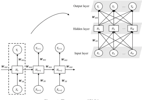
Unlike feedforward neural networks, the recurrent neural network (RNN) can use historical information to help the current decision. RNN mainly uses the neurons with self-feedback to memorize the previous information and applies it to the calculation of the current output. The input of the hidden layer includes not only the input of the input layer at the current time but also the output of the hidden layer at the previous moment. That is, the output of the current time of a sequence is related to the output of the previous time, as shown in Figure1.

Energies 2020, 13, x FOR PEER REVIEW 4 of 21

𝛽 = 𝛽⋮ 𝛽 _× , 𝑻 = 𝒕 ⋮ 𝒕 _× . (5)

In the ELM algorithm, the input weight vector and the bias of the hidden layer can be given randomly. From Equation (4), it can be seen that the hidden layer output matrix, 𝑯, becomes a fixed matrix. At this time, the training of ELM can be translated into seeking the least squares solution of the output weight matrix, 𝛽. The output weight matrix, 𝛽, is calculated by the following formula:

𝛽 = 𝑯 𝑻, (6)

where 𝑯 represents the Moore–Penrose generalized inverse of the hidden layer output matrix, 𝑯.

2.2. Recurrent Neural Network

Unlike feedforward neural networks, the recurrent neural network (RNN) can use historical information to help the current decision. RNN mainly uses the neurons with self-feedback to memorize the previous information and applies it to the calculation of the current output. The input of the hidden layer includes not only the input of the input layer at the current time but also the output of the hidden layer at the previous moment. That is, the output of the current time of a sequence is related to the output of the previous time, as shown in Figure 1.

Figure 1. The structure of RNN.

From Figure 1, we can see that a simple RNN model consists of three layers: The input layer, hidden layer, and output layer, and the connection between the layers is fully connected. Where 𝑊 represents the weight matrix between the input layer and the hidden layer, 𝑊 represents the weight matrix between the previous hidden layer to the current hidden layer, and 𝑊 represents the weight matrix between the hidden layer and the output layer. The weight matrix at each moment is shared, and the expanded RNN can be regarded as a multi-layer feedforward neural network with

parameter sharing. Suppose the input sequence of RNN with length 𝑇 is 𝑋 =

𝑋 , ⋯ , 𝑋 , 𝑋 , 𝑋 , ⋯ , 𝑋 , the dimension of the input data, 𝑋, at each moment is 𝑁, namely 𝑋 =

𝑾 𝑾 𝑾 𝑾 𝑌 𝐻 𝑋 𝑌 𝐻 𝑋 𝑌 𝐻 𝑋 𝑾 𝑾 𝑾 𝑾 𝑾 𝑾 𝑌 𝑌 … 𝑌 𝐻 𝐻 … 𝐻 … 𝑾 𝑾 Output layer Hidden layer Input layer 𝑋 𝑋 𝑋

Figure 1.The structure of RNN.

From Figure1, we can see that a simple RNN model consists of three layers: The input layer, hidden layer, and output layer, and the connection between the layers is fully connected. WhereWIH represents the weight matrix between the input layer and the hidden layer,WHHrepresents the weight

(5)

matrix between the previous hidden layer to the current hidden layer, andWHOrepresents the weight matrix between the hidden layer and the output layer. The weight matrix at each moment is shared, and the expanded RNN can be regarded as a multi-layer feedforward neural network with parameter sharing. Suppose the input sequence of RNN with lengthTisX=

X1,· · ·,Xt,Xt+1,Xt+2,· · ·,XT , the

dimension of the input data,Xt, at each moment isN, namelyXt= (x1,x2,· · ·,xN); the number of

nodes in the hidden layer isM, namelyHt= (h1,h2,· · ·,hM); and the number of nodes in the output

layer isP, namelyYt = (y1,y2,· · ·,yP). Then, the hidden layer,Ht, at timetcan be calculated by

Equations (7) and (8):

Ot=WIHXt+WHHHt−₁+b_h, (7)

Ht= fH(Ot), (8)

where fH(·₎_{is the activation function of the hidden layer and}_b_h_{is the bias vector of the hidden layer. It}

is worth noting that whent=0, that is, when the model starts the first calculation, in order to improve the stability and the overall performance, we usually initializeH0to a number that is relatively small

but not zero [34]. The calculation of the output layer,Yt, at timetcan be obtained by the following equation:

Yt= fO(WHOHt+bo), (9)

where fO(·)is the activation function of the output layer,bois the bias vector of the output layer, and the feedforward process of the model starts fromt=1.

As a model of supervised learning, the training goal of RNN is to minimize the objective function. In order to achieve the training objectives, RNN uses the backpropagation through time (BPTT) [35] to perform gradient calculation on the model to optimize the parameters of RNN.

2.3. Support Vector Machine Given a set of points,M=

(x1,y1),(x2,y2),· · ·,(xn,yn),xn∈Rk.xnis the input feature variable,

which belongs to either of the two categories according to its labelyn∈ {−_1,₊₁}_{. For the nonlinearly}

separable problem, a high-dimensional maximum margin hyperplane can be represented as follows:

y=b+Xω_iyiK(x(i),x), (10)

wherexis the test example,x(i)is the support vector, andK(·)is the kernel function. The kernel function can map low-dimensional feature variables to high-dimensional feature variables. Common choices of the kernel function include the polynomial kernel function and Gaussian radial basis function (RBF).

To obtain an optimal hyperplane, the above problem can be converted into the following quadratic programming (QP) problem: Minimize1₂kωk2₊_CPn i=1ξi Subject to ( yi(ω·φ₍_xi_{) +}_b_{) +}ξ_i≥_1, _i₌_1,· · ·_,_n ξi≥0, i=1,· · · ,n , (11)

whereCis the penalty factor,ξiis the slack variable,·is the dot product,φ(·)is the nonlinear map,ωis the normal vector of the hyperplane, andbis the bias.

2.4. Multi-Objective Particle Swarm Optimization (MOPSO) 2.4.1. Multi-Objective Optimization

For optimization problems that achieve more than one objective function, it is often referred to as multi-objective optimization. The multi-objective optimization problem can be described by the following mathematical form:

(6)

min f(x) = [f1(x),f2(x),· · ·,fn(x)], (12)

subject to (

gi(x)≤_0, _i₌_{1, 2,}· · ·_,_m

hj(x) =0, j=1, 2,· · ·_,_p , (13)

wherex= [x1,x2,· · ·,xn]Trepresents the decision vector, fi(x)i=1, 2,· · ·krepresents thei-th objective

function, andgi(x),hj(x):i=1, 2,· · ·m, j=1, 2,· · ·prepresents the constraints of the target problem, respectively, and finally, the optimal solution of the total target, f(x), should be found. In order to better understand the concept of optimal solutions, this paper introduces the following definition [36]: Definition 1. Pareto dominance.

Given two vectorsx= (x1,x2,· · ·,xt)andy=y1,y2,· · ·,yt,xdominatesy(xy)if:

∀_i∈_[_1,_t_]_, _[_f₍_x_i₎≥ _f₍_y_i_)]∧_[∃_i∈_[_1,_t_]_: _f₍_x_i_)]_. ₍₁₄₎

Definition 2. Pareto optimality.

A pareto-optimalxbelongs toXif:

@y∈Xsubject toF(x)≺F(y). (15)

Definition 3. Pareto optimal set.

Ps :=

x,y∈_X|∃_F₍_x₎≺_F₍_y₎_. ₍₁₆₎

Definition 4. Pareto optimal front.

A set includes the value of objective functions for pareto solutions set:

Pf :=F(x)|x∈Ps . (17)

2.4.2. MOPSO

For the problem of multi-objective function optimization, Moore J et al. [37] first tried to use particle swarm optimization (PSO) to explore multi-objective problems, and then other researchers [38,39] improved the PSO algorithm to solve the multi-objective optimization problem. In 2004, Coello et al. [40] proposed the multi-objective particle swarm optimization (MOPSO) algorithm, which has been widely used in many fields by researchers.

When the PSO algorithm performs single-objective optimization, once the leader in the particle population (the individual optimal solution and the global optimal solution after the last iteration) is determined in each iteration, the search direction is also determined. However, in the optimization process of multi-objective problems, each particle may have multiple different leaders, and one of these leaders needs to be selected to determine the search direction of the particles. In multi-objective optimization, such a group of leaders needs to be stored in a repository, and the repository contains the non-dominated solution set searched so far (generally, its storage location is different from the particle population, called the external archive). In the iterative update of the particle swarm, the algorithm will select the non-dominated solution from the repository as the leader. After the algorithm completes the iterative search, the solution set in the external archive is the output of the algorithm.

(7)

3. Proposed Model

In recent years, many combined methods have been proposed to improve the accuracy and performance of electric load forecasting [41]. The main issue in these combinations is how to connect and combine the models with each other so that they have the desired accuracy of prediction and simultaneously exert the benefits of single-mode models. In this paper, the components of the three artificial neural networks (ANNs) are combined, based on their weight, as follows:

ˆ

YCom,t=W1YˆSVM,t+W2YˆELM,t+W3YˆRNN,t(t=1, 2,· · ·,m), (18) where the forecasted value of the combined model at timetis illustrated by ˆfCom,t,(t=1, 2,· · ·,m);

ˆ

YSVM,t, ˆYELM,t, and ˆYRNN,t are the forecasting results at time t by SVM, ELM, and RNN; and Wi,(i=1, 2, 3)is the weight coefficient allocated to the three ANNs. The weights of each component of

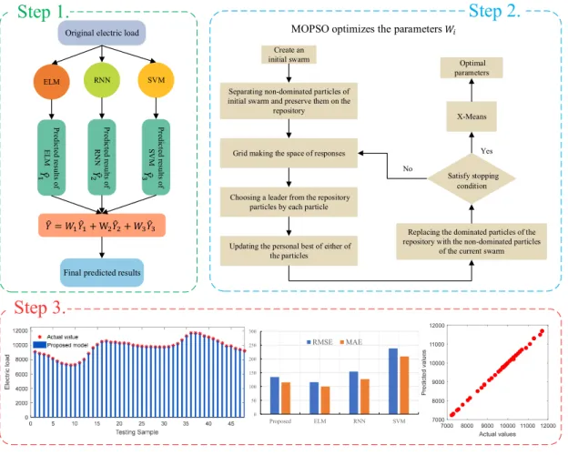
the combined model are calculated in such a way that the error values are minimized. Several different heuristic and meta-heuristic optimization techniques, such as genetic algorithms (GAs), differential evolution (DE), particle swarm optimization (PSO), etc., have been proposed in recent years in order to improve the forecasting performance. However, these methods only consider the accuracy of the combined model. In this paper, MOPSO is used to optimize the weight coefficient, which can not only improve the accuracy but also consider the stability of the combined model. The general flowchart of the proposed model is illustrated in Figure2. From Figure2, we can see that the proposed combined model includes the following three steps.

RNN SVM

ELM

MOPSO optimizes the parameters Create an

initial swarm _Optimal

parameters

Yes

No

Satisfy stopping condition

Final predicted results

Pr ed ic te d r es ult s o f ELM Pr ed ic te d r es ult s o f RN N Pr ed ic te d r es ult s o f SV M

Separating non-dominated particles of initial swarm and preserve them on the

repository

Grid making the space of responses

Choosing a leader from the repository particles by each particle

Updating the personal best of either of the particles

Replacing the dominated particles of the repository with the non-dominated particles

of the current swarm X-Means

Yes

Original electric load

Step 1.

Step 2.

7000 8000 9000 10000 11000 12000 Actual values 7000 8000 9000 10000 11000 12000

Step 3.

𝑌 = 𝑊 𝑌 + W 𝑌 + 𝑊 𝑌 𝑌 𝑌 𝑌 𝑊 0 50 100 150 200 250 300 Proposed ELM RNN SVM RMSE MAE

Figure 2. The flowchart of the proposed model.

Figure 2.The flowchart of the proposed model.

Step 1. Three ANNs, which include ELM, RNN, and SVM, are applied separately to forecast the electric load. After that, combined theory [10] is used to combine the three intermediate forecasting results.

(8)

Step 2. MOPSO is applied to optimize the weight coefficients of the combined model. When using MOPSO to get the optimal weight coefficient, it will get a lot of weights, and each weight is actually a particle. In this paper, X-Means [42] is used to cluster the particles, and then a cluster that contains the most particles is selected. The selected cluster has a center, and the particle closest to the center is the final weight.

Step 3.If the weight coefficient obtained in Step 2 does not reach the expected forecasting result, we continue to use MOPSO to optimize the weight coefficient; otherwise, the final forecasting result can be obtained.

4. Experimental Results and Discussion

In order to verify whether the combined model proposed in this paper can achieve accurate prediction effect when applied to electric load forecasting, the following two experiments were carried out. All the data collected for electric load forecasting in this experiment came from Australia. For the first experiment, three models, including ELM, RNN, and SVM, were used to forecast the electric load independently. In the second experiment, the combined model, which is aimed at improving the accuracy and stability, was applied for multi-step prediction.

4.1. Dataset

The original data used in this article includes three data sets from Australia, which are new data from New South Wales (NSW)) from May 2 2011 to July 3 2011, data from Queensland (QLD)) from April 20 2015 to June 21 2015, and data from Victoria (VIC) from April 30 2007 to July 1 2007. These data sets were obtained based on observation records with a length of two months. In addition, it is composed of data collected by every half hour from 00:00 to 23:30, so 48 observations could be obtained in one day. To test the stability of this model, datasets were collected from Monday to Sunday, so 48 values were obtained every day. Because eight weeks of data were collected, these data were used to predict values for the same day in the next week. Therefore, the dataset was divided into two parts, namely the training set and testing set. Because the data was recorded every half hour, the length of the training data sequence was 2688 (48*8*7), and the length of the testing data sequence was 336 (48*1*7).

For multi-step forecasting, the rolling prediction mechanism was applied in this paper to deal with the input vector every time the input data slides back once. The steps of forecasting minus one was the delayed operator. More specifically, for one-step-ahead forecasting, the delayed operator was 0; for two-steps-ahead forecasting, the delayed operator was 1; and for three-steps-ahead forecasting, the delayed operator was 2. In addition, every time, the output vector was 1. For the SVM and RNN used in this paper, the following parameters were used: The number of hidden layers in RNN was 4, and the regularization parameter and the kernel parameter of SVM were 100 and 0.1, respectively. 4.2. Forecasting Performance Metrics

There is no doubt that there is no perfect model for obtaining the best electric load forecasting performance. In the process of continuously evaluating the prediction results of various models, many evaluation indexes have appeared, but there is no unified standard. Therefore, in order to fully understand the advantages and disadvantages of a model, this paper used the most commonly used three indicators for the evaluation. These are the mean absolute error (MAE), root mean square error (RMSE), and mean absolute percentage error (MAPE), respectively, and the formulas are as follows:

MAE= 1 N n X n=1 |_yn− eyn|, (19) MAPE= 1 N n X n=1 |yn−eyn yn | ×100%, , (20)

(9)

RMSE= 1 N n X n=1 (yn− eyn) 2 , (21)

whereynis the original value andeynis the predicted value, and the smaller the evaluation result value, the higher the accuracy of the model.

4.3. Experimental Results and Analysis

In this section, we first use ELM, RNN, and SVM to predict the electric load, respectively, and then adjust the prediction results by using these models as the three sub-models to construct the combined model. This paper is conducted in two parts: One is the single-model electric load forecasting, which consists of three components; and the other includes a comparison of the forecasting results of the combined model in three datasets against the single models. For the reason that the advantages of the combined model could be shown perfectly, the four forecasting results from New South Wales, Victoria, and Queensland were selected. To put the results in this paper in detail, in this section, the four forecasting models will be described in the following section.

4.3.1. The Forecasting Results of ELM

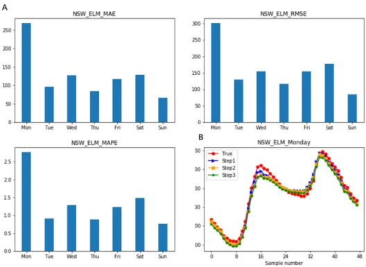
In order to evaluate ELM from various angles, MAE, MAPE, and RMSE were adopted to reveal the effect of ELM. Figure3shows the prediction results of a week. According to the analysis, it can be seen that ELM can achieve a good prediction effect during the week except on Monday, and the best performance is on Sunday. The MAE, MAPE, and RMSE are 66.2811, 0.7571, and 84.2174, respectively. Due to the six days’ good performance, we know that ELM performs well when using this dataset. When looking at the value of Sunday, the forecasting results of the multi-step are shown in Figure3. We can see that compared to the original values and predicted values, the coincidence of the two curves is very high, thus it can be seen that ELM can obtain a good prediction effect.

forecasting results of the combined model in three datasets against the single models. For the reason that the advantages of the combined model could be shown perfectly, the four forecasting results from New South Wales, Victoria, and Queensland were selected. To put the results in this paper in detail, in this section, the four forecasting models will be described in the following section.

4.3.1. The Forecasting Results of ELM

In order to evaluate ELM from various angles, MAE, MAPE, and RMSE were adopted to reveal the effect of ELM. Figure 3 shows the prediction results of a week. According to the analysis, it can be seen that ELM can achieve a good prediction effect during the week except on Monday, and the best performance is on Sunday. The MAE, MAPE, and RMSE are 66.2811, 0.7571, and 84.2174, respectively. Due to the six days’ good performance, we know that ELM performs well when using this dataset. When looking at the value of Sunday, the forecasting results of the multi-step are shown in Figure 3. We can see that compared to the original values and predicted values, the coincidence of the two curves is very high, thus it can be seen that ELM can obtain a good prediction effect.

However, after observing the more detailed data in Table 1, it was found that only three days out of seven days in one-week ELM achieved a better prediction value while the prediction effect of the remaining four days was not ideal, especially as the difference between the predicted value on Monday and the original value was relatively large. Therefore, there is no doubt that we can draw the following conclusions:

(1) ELM can achieve a perfect prediction effect on most days of the week, but it does not have a stable prediction ability.

(2) The prediction effect of ELM on each day is relatively average, being neither good nor bad.

Figure 3. Comparison of the 1-step, 2-step, and 3-step forecasting results of ELM on Monday. (A):

three evaluation metrics results of ELM. (B): ELM forecasting results on Monday.

Figure 3.Comparison of the 1-step, 2-step, and 3-step forecasting results of ELM on Monday. (A): three evaluation metrics results of ELM. (B): ELM forecasting results on Monday.

However, after observing the more detailed data in Table1, it was found that only three days out of seven days in one-week ELM achieved a better prediction value while the prediction effect of

(10)

the remaining four days was not ideal, especially as the difference between the predicted value on Monday and the original value was relatively large. Therefore, there is no doubt that we can draw the following conclusions:

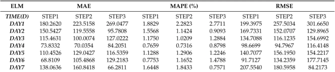
Table 1.One-step, 2-step, and 3-step of the typical results of ELM for a week in NSW.

ELM MAE MAPE (%) RMSE

TIME(D) STEP1 STEP2 STEP3 STEP1 STEP2 STEP3 STEP1 STEP2 STEP3

DAY1 180.2620 223.5158 269.0477 1.8829 2.2823 2.7711 199.3975 257.5034 301.6650 DAY2 150.5427 119.5558 95.7808 1.5568 1.1424 0.9093 169.7331 152.0707 129.8965 DAY3 115.4631 100.0074 127.0222 1.1750 1.0209 1.2884 134.7088 116.1235 154.6992 DAY4 73.8332 70.0354 84.2051 0.7659 0.7316 0.8798 98.6699 94.7967 116.4148 DAY5 110.4526 129.0427 116.5359 1.1288 1.2906 1.2246 140.7077 156.1950 154.2217 DAY6 68.8109 105.4868 129.2183 0.7753 1.1652 1.4788 91.7127 134.2359 177.7145 DAY7 138.0636 160.8418 66.2811 1.6448 1.8433 0.7571 207.5540 180.5958 84.2173

(1) ELM can achieve a perfect prediction effect on most days of the week, but it does not have a stable prediction ability.

(2) The prediction effect of ELM on each day is relatively average, being neither good nor bad. 4.3.2. The Forecasting Results of RNN

Figure4shows the prediction results of the RNN model. Similarly, the performance was also evaluated by MAE, MAPE, and RMSE. As can be seen from part A of Figure4, on the whole, the trend of the predicted results of RNN is similar to ELM, and what impresses us most is that RNN had better predictive values on Thursday than on the other six days. What is more, the RNN model not only performs poorly like ELM on Monday but also has a higher prediction value on Tuesday. In order to estimate the stability of this model intuitively, we used Thursday’s forecasting result as an example. The experimental results on Thursday of RNN are shown in part B of Figure4. Although Thursday represents the best prediction effect of the RNN model, we cannot ignore the fact that the three curves of step 1, step 2, and step 3 on Thursday are not completely consistent with the actual value from the figure.

Table 1. One-step, 2-step, and 3-step of the typical results of ELM for a week in NSW.

ELM MAE MAPE (%) RMSE

4.3.2. The Forecasting Results of RNN

Figure 4 shows the prediction results of the RNN model. Similarly, the performance was also evaluated by MAE, MAPE, and RMSE. As can be seen from part A of Figure 4, on the whole, the trend of the predicted results of RNN is similar to ELM, and what impresses us most is that RNN had better predictive values on Thursday than on the other six days. What is more, the RNN model not only performs poorly like ELM on Monday but also has a higher prediction value on Tuesday. In order to estimate the stability of this model intuitively, we used Thursday's forecasting result as an example. The experimental results on Thursday of RNN are shown in part B of Figure 4. Although Thursday represents the best prediction effect of the RNN model, we cannot ignore the fact that the three curves of step 1, step 2, and step 3 on Thursday are not completely consistent with the actual value from the figure.

In Table 2, we can clearly see each value of the forecasting results of RNN. If the value of MAPE is less than 1.00, the prediction effect of this day is better, and the conditions are met on Thursday and Friday. In addition, the maximum, minimum, and fluctuation of MAE, MAPE, and RMSE can also be observed. Therefore, for the RNN model, the following conclusion can be drawn:

(1) The prediction effect of the RNN model is relatively average, and unacceptable extreme values may occur.

(2) The three evaluation metrics’ values of the RNN model are generally high.

Figure 4. Comparison of the 1-step, 2-step, and 3-step forecasting results of RNN on Thursday. (A):

three evaluation metrics results of RNN (B): RNN forecasting results on Thursday.

Figure 4.Comparison of the 1-step, 2-step, and 3-step forecasting results of RNN on Thursday. (A): three evaluation metrics results of RNN (B): RNN forecasting results on Thursday.

(11)

In Table2, we can clearly see each value of the forecasting results of RNN. If the value of MAPE is less than 1.00, the prediction effect of this day is better, and the conditions are met on Thursday and Friday. In addition, the maximum, minimum, and fluctuation of MAE, MAPE, and RMSE can also be observed. Therefore, for the RNN model, the following conclusion can be drawn:

Table 2.One-step, 2-step, and 3-step of the typical results of RNN for a week in NSW.

RNN MAE MAPE (%) RMSE

(1) The prediction effect of the RNN model is relatively average, and unacceptable extreme values may occur.

(2) The three evaluation metrics’ values of the RNN model are generally high. 4.3.3. The Forecasting Results of SVM

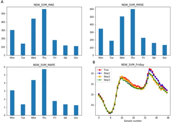
In part A of Figure5, the prediction results obtained using SVM in NSW are displayed. According to the bar chart in Figure5, the performance of Tuesday, Friday, Saturday, and Sunday is better, in which the best one of the four days can be obtained in a week. Besides, no one can deny the fact that the forecasting result of Wednesday was very unsatisfactory. In order to highlight the gap between the original value and the predicted value, it can be clearly seen from part B of Figure5that the predicted result of SVM on Friday almost coincides with the curve of the original data. On the one hand, we can see when the accuracy at all the moments is the highest. On the other hand, we can see that the curve of SVM was less consistent with the actual data at a specific time point

Table 2. One-step, 2-step, and 3-step of the typical results of RNN for a week in NSW.

RNN MAE MAPE (%) RMSE

DAY1 204.1581 100.5311 101.6679 2.0580 1.0004 1.0509 213.0676 161.3429 110.6075 DAY2 98.1426 167.0452 122.8477 0.9296 1.6683 1.1735 134.0583 182.9610 160.6650 DAY3 121.8523 72.2479 97.6225 1.2474 0.7655 1.0284 139.6238 85.7970 118.0915 DAY4 67.4409 67.5249 82.0695 0.6929 0.7009 0.8547 93.1168 93.0551 113.8564 DAY5 114.3743 95.8134 92.7150 1.1588 0.9740 0.9485 136.1701 113.4121 114.0553 DAY6 76.4809 109.1112 109.3341 0.8619 1.2323 1.2266 103.1139 136.8135 129.6750 DAY7 110.8216 82.7990 121.9677 1.2929 1.0041 1.3783 130.8743 114.4017 153.7139 4.3.3. The Forecasting Results of SVM

In part A of Figure 5, the prediction results obtained using SVM in NSW are displayed. According to the bar chart in Figure 5, the performance of Tuesday, Friday, Saturday, and Sunday is better, in which the best one of the four days can be obtained in a week. Besides, no one can deny the fact that the forecasting result of Wednesday was very unsatisfactory. In order to highlight the gap between the original value and the predicted value, it can be clearly seen from part B of Figure 5 that the predicted result of SVM on Friday almost coincides with the curve of the original data. On the one hand, we can see when the accuracy at all the moments is the highest. On the other hand, we can see that the curve of SVM was less consistent with the actual data at a specific time point

From Table 3, we can see that the SVM model does not behave well on one day, as the lowest value of MAPE is 1.2377 on Sunday and the highest value of MAPE is 5.7218 on Thursday. Meanwhile, the value of MAE and RMSE can be easily observed.

Figure 5. Comparison of the 1-step, 2-step, and 3-step forecasting results of SVM on Friday. (A): three evaluation metrics results of SVM. (B): SVM forecasting results on Friday.

Figure 5.Comparison of the 1-step, 2-step, and 3-step forecasting results of SVM on Friday. (A): three evaluation metrics results of SVM. (B): SVM forecasting results on Friday.

(12)

From Table3, we can see that the SVM model does not behave well on one day, as the lowest value of MAPE is 1.2377 on Sunday and the highest value of MAPE is 5.7218 on Thursday. Meanwhile, the value of MAE and RMSE can be easily observed.

Table 3.One-step, 2-step, and 3-step of the typical results of SVM for a week in NSW.

SVM MAE MAPE (%) RMSE

4.3.4. The Forecasting Results of Combined

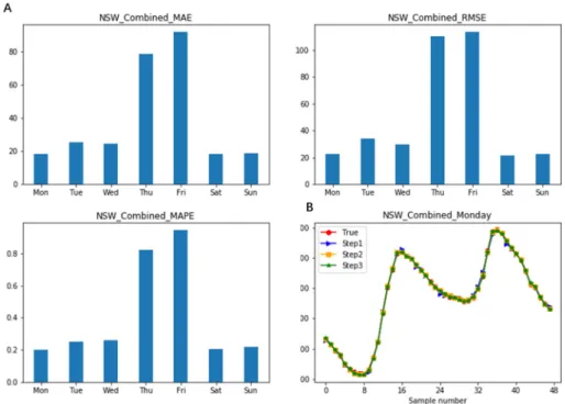
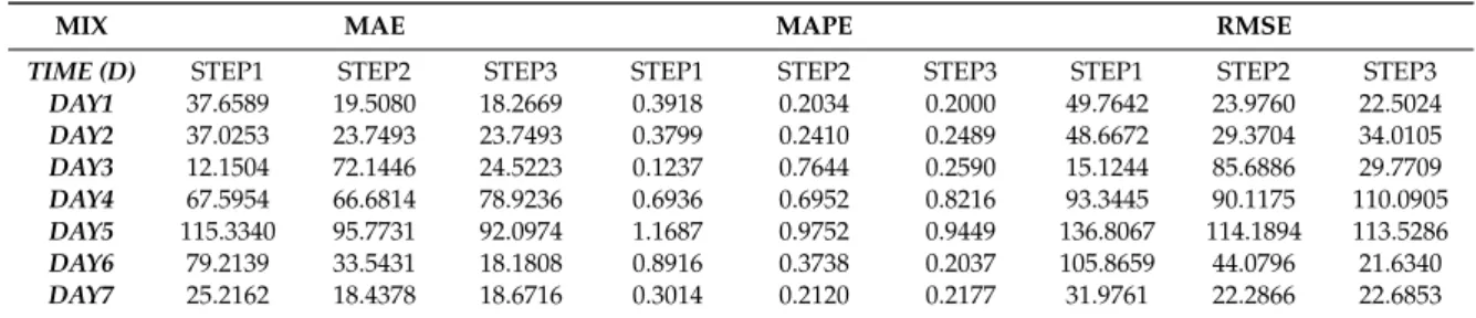
To further show that the combined model could capture the characteristics of each model effectively, the performance of the proposed model, which consists of ELM, RNN, and SVM, is displayed in this part. Firstly, we cannot ignore the fact that the three forecasting metric values (MAE, MAPE, and RMSE) of the three ANNs on Friday are very high, which also means that the result of the combined model on Friday is not accurate. After carefully observing part A of Figure6, we can see that the three performance metrics are very average expect on Friday, and Figure6also shows that there is no negative value. From part B of Figure6, we can directly know that there is almost no gap between the original value and the predicted value on Monday. Unlike NSW, SVM can perform well in local optimization, and the combined model performs good in all 48 moments. The performance of the combined model for each day is presented in Table4. All values of MAPE are much smaller than the lower limits at 0.30, and the maximum value is also below 1.00.

Table 3. One-step, 2-step, and 3-step of the typical results of SVM for a week in NSW.

SVM MAE MAPE (%) RMSE

4.3.4. The Forecasting Results of Combined

To further show that the combined model could capture the characteristics of each model effectively, the performance of the proposed model, which consists of ELM, RNN, and SVM, is displayed in this part. Firstly, we cannot ignore the fact that the three forecasting metric values (MAE, MAPE, and RMSE) of the three ANNs on Friday are very high, which also means that the result of the combined model on Friday is not accurate. After carefully observing part A of Figure 6, we can see that the three performance metrics are very average expect on Friday, and Figure 6 also shows that there is no negative value. From part B of Figure 6, we can directly know that there is almost no gap between the original value and the predicted value on Monday. Unlike NSW, SVM can perform well in local optimization, and the combined model performs good in all 48 moments. The performance of the combined model for each day is presented in Table 4. All values of MAPE are much smaller than the lower limits at 0.30, and the maximum value is also below 1.00.

When evaluating these four models (ELM, RNN, SVM, and the combined model) systematically, it is very obvious that the prediction effect of the combined model is superior to the three classic models by using the same dataset of NSW. Compared with the other three models, the combined model can obtain the minimum MAPE, with a value of 0.20.

Figure 6. Comparison of the 1-step, 2-step, and 3-step forecasting results of the combined model on

Monday. (A): three evaluation metrics results of Combined model. (B): Combined model forecasting

results on Monday.

Figure 6.Comparison of the 1-step, 2-step, and 3-step forecasting results of the combined model on Monday. (A): three evaluation metrics results of Combined model. (B): Combined model forecasting results on Monday.

(13)

Table 4.One-step, 2-step, and 3-step of the typical results of the combined model for a week in NSW.

MIX MAE MAPE RMSE

TIME (D) STEP1 STEP2 STEP3 STEP1 STEP2 STEP3 STEP1 STEP2 STEP3

When evaluating these four models (ELM, RNN, SVM, and the combined model) systematically, it is very obvious that the prediction effect of the combined model is superior to the three classic models by using the same dataset of NSW. Compared with the other three models, the combined model can obtain the minimum MAPE, with a value of 0.20.

4.3.5. The Forecasting Results of the Four Models and Comparisons

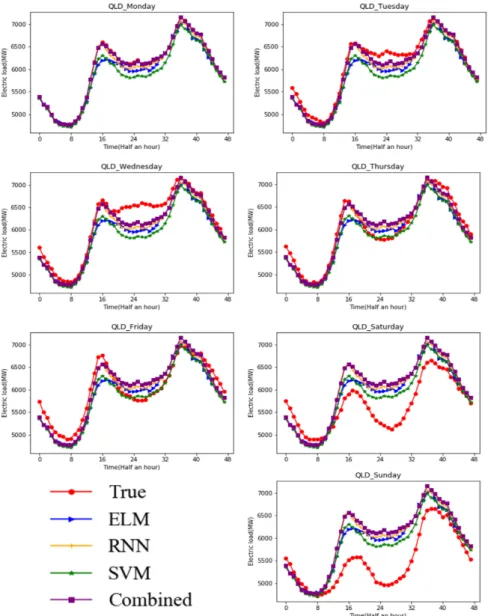
In this subsection, a holistic comparison with the other three methods (ELM, RNN, and SVM) is conducted to estimate the effectiveness of the combined model by putting it under broader time and space conditions. Generally speaking, the combined model has a stronger capability to forecast the electric load than the other three models. Figure7shows the prediction values and original values for the seven days of all four models in Queensland. As is vividly shown in the graph, the five curves are representative of the different values. These curves with different colors stand for electric load values by ELM, RNN, SVM, and the combined model, respectively. From Figure7, there is no doubt that every model can get the best result in some special time points. Among the four models, it is noteworthy that the combined model curve is less consistent with the actual values while the ELM and RNN curves are more consistent with the actual values, with between 15 and 38 time points in one day expect on Monday. From the curves, it can be recognized that the combined model curve and the actual curve almost overlap. However, when we look at the curves on Saturday and Sunday, we could draw a conclusion that the four models only achieve better prediction in the first 10 observations. So, in order to more thoroughly estimate which model can achieve the best forecasting results synthetically, the results taking the three forecasting metrics (MAE, MAPE, and RMSE) into account are recorded in Table5.

Table5reveals the calculated values of three evaluation metrics and the average values of four models for a week in Queensland. In order to compare the four models in detail, we considered MAE, RMSE, and MAPE to estimate which model had the best performance. When we contrasted the combined model with the other three models, the results were as follows.

Table 5.Results of the three evaluation metrics of the four models for Queensland.

Date Monday Tuesday Wednesday Thursday Friday Saturday Sunday Average

MAE ELM 106.7967 430.4047 124.4383 248.7430 137.0113 119.1218 232.6718 199.8839 RNN 49.4061 51.9644 96.5393 105.4656 135.3078 114.5491 132.4774 97.9585 SVM 169.2212 130.8537 74.2149 223.3669 210.5455 139.9597 202.0815 164.3205 Combined 10.3468 45.7838 51.5260 79.4087 103.8398 17.2876 122.8888 61.5831 RMSE ELM 146.4229 622.5072 195.6884 329.6401 206.9160 177.1841 330.4177 286.9681 RNN 61.1178 78.9962 129.8775 141.4667 188.2211 153.6274 189.4702 134.6824 SVM 196.0913 169.0187 106.3683 340.2963 328.5419 215.5059 308.1820 237.7149 Combined 13.5202 60.0425 79.8899 98.0779 133.2788 25.3522 172.3644 83.2180 MAPE (%) ELM 1.6979 6.6900 1.9441 4.1041 2.2723 2.1641 4.3466 3.3170 RNN 0.7952 0.8301 1.5119 1.7711 2.2433 2.0834 2.4881 1.6747 SVM 2.7228 2.0697 1.1872 3.7387 3.5043 2.5591 3.8490 2.8044 Combined 0.1681 0.7346 0.8177 1.3294 1.7087 0.3037 2.2958 1.0511

(14)

The combined model vs, ELM, RNN, and SVM: Compared with the other three models, the presented combined model, which contains the lowest MAE, MAPE, and RMSE values in the days of the week, can still get the lowest average values, which means the combined model is suitable for forecasting the electric load in Queensland. In addition, the MAPE of the combined model is not more than 0.15 and is also less than 3.00. When compared with ELM, it could be observed that the great improvements on the forecasting effectiveness of the proposed model are fairly obvious. To be frank, the combined model achieved the maximum improvement of MAE, RMSE, and MAPE, which are 69.19%, 71.00%, and 68.37%, respectively. Similarly, when compared with RNN, the combined model achieved the minimum improvement of MAE, RMSE, and MAPE, which are 37.13%, 38.21%, and 37.28%. At last, a comparison with SVM was made, revealing that combined model reduced MAE by 62.52%, RMSE by 64.99%, and MAPE by 62.5%. In the following, the merits and demerits of the three models are recommended.Energies 2020, 13, x FOR PEER REVIEW 15 of 21

Figure 7. Comparison of forecasting performances of four models for Queensland in a week.

Table 5. Results of the three evaluation metrics of the four models for Queensland.

Date Monday Tuesday Wednesday Thursday Friday Saturday Sunday Average MAE ELM 106.7967 430.4047 124.4383 248.7430 137.0113 119.1218 232.6718 199.8839 RNN 49.4061 51.9644 96.5393 105.4656 135.3078 114.5491 132.4774 97.9585 SVM 169.2212 130.8537 74.2149 223.3669 210.5455 139.9597 202.0815 164.3205 Combined 10.3468 45.7838 51.5260 79.4087 103.8398 17.2876 122.8888 61.5831 RMSE ELM 146.4229 622.5072 195.6884 329.6401 206.9160 177.1841 330.4177 286.9681

Figure 7.Comparison of forecasting performances of four models for Queensland in a week.

RNN vs. ELM and SVM: The three metrics of MAE, RMSE and MAPE of RNN have lower values than ELM and SVM expect on Wednesday. In general, in terms of the average value, RNN is better than ELM and SVM. Even so, compared with ELM, RNN led to a 50.99%, 53.06%, and 49.70% reduction in terms of MAE, RMSE, and MAPE. Compared with SVM, RNN reduced MAE by 40.39%, RMSE by 43.34%, and MAPE by 40.36%.

(15)

SVM vs. ELM: It is evident that the forecasting results based on the three error metrics (MAE, RMSE, and MAPE) of SVM are more precise than ELM except on Monday, Friday, and Saturday. Though there are three days of MAE, RMSE and MAPE of ELM are lower than SVM. Compared with the average values, SVM reduced MAE by 17.79%, RMSE by 17.16%, and MAPE by 15.66%.

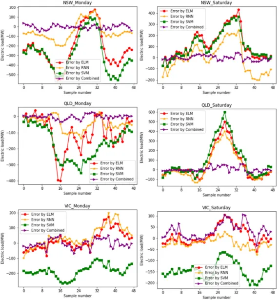
To further illustrate the quality of the entire models, Figure8shows the errors, which are the differences between the actual values and the forecasting values of the four models in New South Wales, Queensland, and Victoria on Monday and Saturday. Though the error rates of the forecasting results are shown in three different sites on Monday, it can obviously be observed that the combined model curve is almost zero and as smooth as a line. On the one hand, that is to say, the combined model obtained the smallest errors with the original values. On the other hand, we can draw the conclusion that the performance of the combined model is remarkably steady overall. The error of the other three models has a great fluctuation range between the positive value of 600 and negative value of 500, among which errors of RNN are almost a line, but all error nodes are under zero. The curves of ELM and SVM fluctuate up and down irregularly. As mentioned above, the smaller the errors are, the better the model is. To sum up, the combined model has the best performance among the four approaches. This demonstrates that the combined model has high accuracy and stability.Energies 2020, 13, x FOR PEER REVIEW 17 of 21

Figure 8. Comparison of the final forecasting errors of the four models on Monday and Saturday.

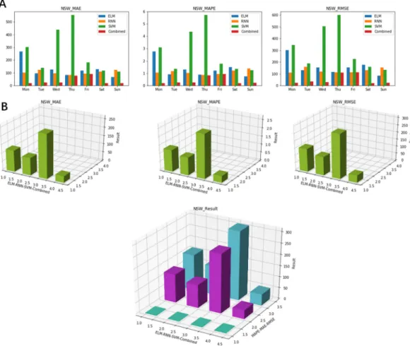
At last, based on the analysis of the previous results, the final prediction effect of the four models is visible in Figure 9. The histogram, in terms of the total forecasting metrics of these four models for a week, is presented in Figure 9 part A in detail. The shorter the histogram is, the better the model is. It is intuitive that the red histogram of the combined model is the shortest, which means the combined model performs well. Based on the above results, we can obtain the final evaluation results (MAE, RMSE, and MAPE) from Figure 9 part B. In Figure 9 part B, 1 represents the result of ELM, 2 shows the result of RNN, 3 is the symbol of SVM, and 4 displays the combined model. From Figure 9 part B, firstly, we can see that the MAE, MAPE, and RMSE of the combined model are the shortest. Then, in the last histogram, the difference among the four models can be seen intuitively. The two parts of Figure 9 together reveal that it is important to generate forecasts in terms of forecasting accuracy and stability for a model in a week. It is worth noting that the mean value of the combined model is lower than the three individual models by the forecasting metrics. We can see the differences vividly in Figure 9.

In a word, based on prior results, the proposed combined model can effectively forecast the electric load with a high prediction performance and strong stability.

(16)

At last, based on the analysis of the previous results, the final prediction effect of the four models is visible in Figure9. The histogram, in terms of the total forecasting metrics of these four models for a week, is presented in Figure9part A in detail. The shorter the histogram is, the better the model is. It is intuitive that the red histogram of the combined model is the shortest, which means the combined model performs well. Based on the above results, we can obtain the final evaluation results (MAE, RMSE, and MAPE) from Figure9part B. In Figure9part B, 1 represents the result of ELM, 2 shows the result of RNN, 3 is the symbol of SVM, and 4 displays the combined model. From Figure9part B, firstly, we can see that the MAE, MAPE, and RMSE of the combined model are the shortest. Then, in the last histogram, the difference among the four models can be seen intuitively. The two parts of Figure9together reveal that it is important to generate forecasts in terms of forecasting accuracy and stability for a model in a week. It is worth noting that the mean value of the combined model is lower than the three individual models by the forecasting metrics. We can see the differences vividly in Figure9.

Figure 9. Comparison of the final forecasting value results of the four models for Queensland in a week.

5. Conclusions

Accurate and stable forecasting results can not only help consumers to save the cast using in electricity but also provide assistance to suppliers to estimate electricity consumption in advance, thus achieving huge economic and social benefits for consumers and suppliers. With respect to the forecasting methods, there is no denying that some approaches cannot be adopted in practice. Furthermore, every single model has inevitable drawbacks, and the combined model takes full advantage of each single model and reduces the negative effects of the individual model.

In this paper, to overcome these drawbacks, this research proposed a novel combined model, which is based on a combination of ELM, RNN, and SVM and employed multi-objective particle swarm optimization (MOPSO). The combined model first used three ANNs, which include ELM, RNN, and SVM, separately to forecast the electric load. Then, the three intermediate forecasting results were obtained. After that, the MOPSO was applied to optimize the weight coefficients of the integrated model for multi-step electric load forecasting. If the weight coefficient could not achieve better results, we continued to use MOPSO to select the weight coefficient, so it is not surprising that the combined model obtained a good prediction result. Considering the time and environmental factors, by simulating the electric load data of three sites from Australia and comparing the combined model with the other three single methods, we found that the behavior of the proposed combined model was superior to the individual model. All in all, the combined model showed great progress in accuracy and stability.

Author Contributions: Conceptualization, Z.S. and Y.C. (Yao Chen); Methodology, Z.S.; Software, Y.Y.; Validation, Y.C. (Yao Chen), Y.C. (Yanhua Chen); Formal Analysis, Z.S. and Y.C. (Yanhua Chen); Investigation,

Figure 9.Comparison of the final forecasting value results of the four models for Queensland in a week.

In a word, based on prior results, the proposed combined model can effectively forecast the electric load with a high prediction performance and strong stability.

5. Conclusions

Accurate and stable forecasting results can not only help consumers to save the cast using in electricity but also provide assistance to suppliers to estimate electricity consumption in advance, thus achieving huge economic and social benefits for consumers and suppliers. With respect to the forecasting methods, there is no denying that some approaches cannot be adopted in practice. Furthermore, every single model has inevitable drawbacks, and the combined model takes full advantage of each single model and reduces the negative effects of the individual model.

(17)

In this paper, to overcome these drawbacks, this research proposed a novel combined model, which is based on a combination of ELM, RNN, and SVM and employed multi-objective particle swarm optimization (MOPSO). The combined model first used three ANNs, which include ELM, RNN, and SVM, separately to forecast the electric load. Then, the three intermediate forecasting results were obtained. After that, the MOPSO was applied to optimize the weight coefficients of the integrated model for multi-step electric load forecasting. If the weight coefficient could not achieve better results, we continued to use MOPSO to select the weight coefficient, so it is not surprising that the combined model obtained a good prediction result. Considering the time and environmental factors, by simulating the electric load data of three sites from Australia and comparing the combined model with the other three single methods, we found that the behavior of the proposed combined model was superior to the individual model. All in all, the combined model showed great progress in accuracy and stability.

Author Contributions:Conceptualization, Z.S. and Y.C. (Yao Chen); Methodology, Z.S.; Software, Y.Y.; Validation, Y.C. (Yao Chen), Y.C. (Yanhua Chen); Formal Analysis, Z.S. and Y.C. (Yanhua Chen); Investigation, Y.C. (Yanhua Chen); Resources, Y.Y.; Data Curation, Y.C. (Yao Chen); Writing-Original Draft Preparation, Z.S.; Writing-Review & Editing, Z.S. and Y.Y.; Visualization, Z.S. and Y.C. (Yao Chen); Supervision, Y.C. (Yanhua Chen); Project Administration, Y.Y.; Funding Acquisition, Y.Y. All authors have read and agreed to the published version of the manuscript.

Funding:This research is supported by National Key R&D Program of China (Grant number 2018YFB1003205, 2017YFE0111900) and 2019 Gansu key talent project.

Conflicts of Interest:The authors declare that there is no conflict of interest regarding the publication of this paper.

References

1. Zhang, J.; Wei, Y.M.; Li, D.; Tan, Z.; Zhou, J. Short term electricity load forecasting using a hybrid model.

Energy2018,158, 774–781. [CrossRef]

2. Velsink, H. Time Series Analysis of 3D Coordinates Using Nonstochastic Observations.J. Appl. Geod.2016,

10, 5–16. [CrossRef]

3. Meng, M.; Wang, L.; Shang, W. Decomposition and forecasting analysis of China’s household electricity consumption using three-dimensional decomposition and hybrid trend extrapolation models.Energy2018,

165, 143–152. [CrossRef]

4. Yunishafira, A. Determining the Appropriate Demand Forecasting Using Time Series Method: Study Case at Garment Industry in Indonesia.KnE Soc. Sci.2018,3, 553–564. [CrossRef]

5. Verma, A.; Karan, A.; Mathur, A.; Chethan, S. Analysis of time-series method for demand forecasting.J. Eng. Appl. Sci.2017,12, 3102–3107.

6. An, Y.; Zhou, Y.; Li, R. Forecasting India’s Electricity Demand Using a Range of Probabilistic Methods.

Energies2019,12, 2574. [CrossRef]

7. Shah, I.; Iftikhar, H.; Ali, S.; Wang, D. Short-Term Electricity Demand Forecasting Using Components Estimation Technique.Energies2019,12, 2532. [CrossRef]

8. Al-Musaylh, M.S.; Deo, R.C.; Adamowski, J.F.; Li, Y. Short-term electricity demand forecasting with MARS, SVR and ARIMA models using aggregated demand data in Queensland, Australia.Adv. Eng. Inf.2018,35, 1–16. [CrossRef]

9. Yixian, L.I.U.; Roberts, M.C.; Sioshansi, R. A vector autoregression weather model for electricity supply and demand modeling.J. Mod. Power Syst. Clean Energy2018,6, 763–776.

10. Yang, Y.; Chen, Y.; Wang, Y. Modelling a combined method based on ANFIS and neural network improved by DE algorithm: A case study for short-term electricity demand forecasting.Appl. Soft Comput.2016,49, 663–675. [CrossRef]

11. Al-Musaylh, M.S.; Deo, R.C.; Li, Y. Two-phase particle swarm optimized-support vector regression hybrid model integrated with improved empirical mode decomposition with adaptive noise for multiple-horizon electricity demand forecasting.Appl. Energy2018,217, 422–439. [CrossRef]

12. Hatori, T.; Sato-Ilic, M. A Fuzzy Clustering Method Using the Relative Structure of the Belongingness of Objects to Clusters.Procedia Comput. Sci.2014,35, 994–1002. [CrossRef]

(18)

13. Majkowski, A.; Kołodziej, M.; Rak, R.J. Joint Time-Frequency and Wavelet Analysis—An Introduction.Metrol. Meas. Syst.2014,21, 741–758. [CrossRef]

14. Bento, P.M.R.; Pombo, J.A.N.; Calado, M.R.A. A bat optimized neural network and wavelet transform approach for short-term price forecasting.Appl. Energy2018,210, 88–97. [CrossRef]

15. Koroglu, S.; Sergeant, P.; Umurkan, N. Comparison of Analytical, Finite Element and Neural Network Methods to Study Magnetic Shielding.Simul. Model. Pract. Theory2010,18, 206–216. [CrossRef]

16. Johannesen, N.J.; Kolhe, M.; Goodwin, M. Relative evaluation of regression tools for urban area electrical energy demand forecasting.J. Clean. Prod.2019,218, 555–564. [CrossRef]

17. Trull,Ó.; García-Díaz, J.C.; Troncoso, A. Application of Discrete-Interval Moving Seasonalities to Spanish Electricity Demand Forecasting during Easter.Energies2019,12, 1083. [CrossRef]

18. Ceci, M.; Corizzo, R.; Malerba, D. Spatial autocorrelation and entropy for renewable energy forecasting.Data Min. Knowl. Discov.2019,33, 698–729. [CrossRef]

19. La Rosa, M.; Rabinovich, M.I.; Huerta, R. Slow regularization through chaotic oscillation transfer in an unidirectional chain of Hindmarsh–Rose models.Phys. Lett. A2000,266, 88–93. [CrossRef]

20. Yang, A.; Li, W.; Yang, X. Short-term electricity load forecasting based on feature selection and Least Squares Support Vector Machines.Knowl. Based Syst.2019,163, 159–173. [CrossRef]

21. Bedi, J.; Toshniwal, D. Deep learning framework to forecast electricity demand. Appl. Energy2019,238, 1312–1326. [CrossRef]

22. Eseye, A.T.; Lehtonen, M.; Tukia, T. Machine learning based integrated feature selection approach for improved electricity demand forecasting in decentralized energy systems.IEEE Access2019,7, 91463–91475. [CrossRef]

23. Liu, P.; Zheng, P.; Chen, Z. Deep Learning with Stacked Denoising Auto-Encoder for Short-Term Electric Load Forecasting.Energies2019,12, 2445. [CrossRef]

24. Singh, S.; Yassine, A. Big data mining of energy time series for behavioral analytics and energy consumption forecasting.Energies2018,11, 452. [CrossRef]

25. Corizzo, R.; Pio, G.; Ceci, M. DENCAST: Distributed density-based clustering for multi-target regression.J. Big Data2019,6, 43. [CrossRef]

26. Shi, J.; Guo, J.; Zheng, S. Evaluation of hybrid forecasting approaches for wind speed and power generation time series.Renew. Sustain. Energy Rev.2012,16, 3471–3480. [CrossRef]

27. Foley, A.M.; Leahy, P.G.; Marvuglia, A. Current methods and advances in forecasting of wind power generation.Renew. Energy2012,37, 1–8. [CrossRef]

28. Li, S.; Wang, P.; Goel, L. Short-term load forecasting by wavelet transform and evolutionary extreme learning machine.Electr. Power Syst. Res.2015,122, 96–103. [CrossRef]

29. Zhang, X.; Wang, J.; Zhang, K. Short-term electric load forecasting based on singular spectrum analysis and support vector machine optimized by Cuckoo search algorithm.Electr. Power Syst. Res.2017,146, 270–285. [CrossRef]

30. Xiao, L.; Wang, J.; Hou, R. A combined model based on data pre-analysis and weight coefficients optimization for electrical load forecasting.Energy2015,82, 524–549. [CrossRef]

31. Wang, J.; Zhu, S.; Zhang, W. Combined modeling for electric load forecasting with adaptive particle swarm optimization.Energy2010,35, 1671–1678. [CrossRef]

32. Liu, T.; Jin, Y.; Gao, Y. A New Hybrid Approach for Short-Term Electric Load Forecasting Applying Support Vector Machine with Ensemble Empirical Mode Decomposition and Whale Optimization.Energies2019,12, 1520. [CrossRef]

33. Zhang, Y.; Wang, J.; Lu, H. Research and Application of a Novel Combined Model Based on Multiobjective Optimization for Multistep-Ahead Electric Load Forecasting.Energies2019,12, 1931. [CrossRef]

34. Sutskever, I.; Martens, J.; Dahl, G. On the importance of initialization and momentum in deep learning.Proc. Mach. Learn. Res.2013,28, 1139–1147.

35. Werbos, P.J. Backpropagation through time: What it does and how to do it.Proc. IEEE1990,78, 1550–1560. [CrossRef]

36. Jin, Y.; Sendhoff, B. Pareto-based multiobjective machine learning: An overview and case studies.IEEE Trans. Syst. Man Cybern. Part C2008,38, 397–415.

37. Moore, J. Application of Particle Swarm to Multiobjective Optimization; Technical Report; Department of Computer Science and Software Engineering, Auburn University: Auburn, AL, USA, 1999.

(19)

38. Bartz-Beielstein, T.; Limbourg, P.; Mehnen, J. Particle Swarm Optimizers for Pareto Optimization with Enhanced Archiving Techniques. In Proceedings of the 2003 Congress on Evolutionary Computation (CEC’03 IEEE), Canberra, Australia, 8–12 December 2003; Volume 3, pp. 1780–1787.

39. Pulido, G.T.; Coello, C.A.C. Using Clustering Techniques to Improve the Performance of a Multi-Objective Particle Swarm Optimizer. InGenetic and Evolutionary Computation Conference; Springer: Berlin/Heidelberg, Germany, 2004; pp. 225–237.

40. Coello, C.A.C.; Pulido, G.T.; Lechuga, M.S. Handling multiple objectives with particle swarm optimization.

IEEE Trans. Evol. Comput.2004,8, 256–279. [CrossRef]

41. Tian, C.; Hao, Y. A novel nonlinear combined forecasting system for short-term load forecasting.Energies 2018,11, 712. [CrossRef]

42. Pelleg, D.; Moore, A.X-Means: Extending K-Means with Efficient Estimation of the Number of Clusters; Morgan Kaufmann Publishers Inc.: San Francisco, CA, USA, 2000.

©2020 by the authors. Licensee MDPI, Basel, Switzerland. This article is an open access article distributed under the terms and conditions of the Creative Commons Attribution (CC BY) license (http://creativecommons.org/licenses/by/4.0/).