Dominik Schreiber
, Damien Pellier
, Humbert Fiorino
and Tom´aˇs Balyo
1Karlsruhe Institut f¨ur Technologie, Karlsruhe, Germany
2Universit´e Grenoble-Alpes, Grenoble, France
Keywords: HTN Planning, SAT Planning, Incremental SAT Solving.
Abstract: Hierarchical Task Networks (HTN) are one of the most expressive representations for automated planning problems. On the other hand, in recent years, the performance of SAT solvers has been drastically improved. To take advantage of these advances, we investigate how to encode HTN problems as SAT problems. In this paper, we propose two new encodings: GCT (Grammar-Constrained Tasks) and SMS (Stack Machine Simulation), which, contrary to previous encodings, address recursive task relationships in HTN problems. We evaluate both encodings on benchmark domains from the International Planning Competition (IPC), setting a new baseline in SAT planning on modern HTN domains.
1
INTRODUCTION
HTN (Hierarchical Task Network) planning (Georgievski and Aiello, 2015) is one of the most efficient and widely used planning techniques
in practice. It is based on expressive languages
allowing to specify complex expert knowledge for real world domains. Unlike classical planning (Fikes and Nilsson, 1971), in HTN planning, the goal is expressed as a set of tasks to achieve, and to which it is possible to associate different kinds of constraints: the set of constraints and tasks is aTask Network.
Boolean satisfiability (SAT) solving is a generic problem resolution method which has already been successfully applied to classical planning before, e.g., (Rintanen, 2012). Given a propositional logic for-mulaF, the objective of SAT solving is to find an assignment to all occurring Boolean variables such thatFevaluates totrue, or to report unsatisfiability if no such assignment exists. When applying SAT solv-ing to plannsolv-ing problems, the full procedure features four steps: (1) enumerating and instantiating all the possible actions, (2) encoding the instantiated plan-ning problem into propositional logic, (3) finding a solution with a SAT solver, e.g., (E´en and S¨orensson, 2003a; Audemard and Simon, 2009; Biere, 2013), and (4) decoding the found variable assignment back to a valid plan. In conventional SAT planning (Kautz and Selman, 1992; Kautz et al., 1996), each fact and each action at each step is commonly represented by a Boolean variable. The logic of how actions are
ex-ecuted and how they transform the world state is en-coded with general clauses, while the initial state and the goal are provided as single literals (unit clauses). As the number of necessary actions is generally un-known in advance, the planning problem is iteratively re-encoded for a growing amount of steps, until a so-lution is found or the computation timed out. The SAT approach to planning is appealing because all planning is performed by SAT solvers using very ef-ficient domain-independent heuristics; thus, any ad-vances towards more efficient SAT solvers can also improve SAT-based planning.
The technique of incremental SAT solving has
recently gained popularity for planning purposes (Gocht and Balyo, 2017). While conventional SAT solving processes a single formula in an isolated manner, incremental SAT solving allows for multiple solving steps while successively modifying the for-mula (E´en and S¨orensson, 2003b): New clauses can be added between steps, and single literals can be as-sumed, i.e. they are enforced for a single solving at-tempt and dropped afterwards. A central advantage of incremental SAT solving is that SAT solvers can learn conflicts in assignments from past solving attempts and thus find a solution more efficiently (Nabeshima et al., 2006).
Compared to classical planning, significantly less research has been done on using SAT solvers for HTN planning (Mali and Kambhampati, 1998). One of the reasons is that enumerating and instantiating methods in HTN planning is challenging. Recently, efficient
Schreiber D., Pellier D., Fiorino H. and Balyo T. Efficient SAT Encodings for Hierarchical Planning. DOI: 10.5220/0007343305310538
instantiation procedures in HTN planning have been proposed (Ramoul et al., 2017), which allows us to investigate effective SAT-based approaches.
In this paper, our contributions are two new SAT encodings for HTN problems: GCT (Grammar-Constrained Tasks) and SMS (Stack Machine Sim-ulation). Contrary to previous encodings (Mali and Kambhampati, 1998), GCT and SMS fully address re-cursive task relationships in HTN problems, and SMS is specifically designed for incremental SAT solving.
2
HTN PLANNING
In this section we introduce the foundations of HTN
planning. A fact is an atomic logical proposition.
A state s is a consistent set of positive facts. An
operator o is a tuple o = (name(o),pre(o), eff(o))
where:name(o)is a syntactic expression of the form
n(x1, . . . ,xn)with n being the name of the operator
andx1, . . . ,xn its parameters; and pre(o)and eff(o)
are two sets of facts which define respectively the pre-conditions that must hold to apply the operator and the effects that must hold after the application ofo.
Anactionis a ground operator, i.e. it has no free
parameters. Action a is applicable to a state s if
pre(a)⊆s. The resulting states0 of the application ofain a state sis defined as follows: s0=γ(s,a) = (s\eff−(a))∪eff+(a), whereeff+(eff−) represent the positive (negative) facts ineff. The application of a se-quence of actions is recursively defined byγ(s,hi) =s andγ(s,ha0,a1, . . . ,ani) =γ(γ(s,a0),ha1, . . . ,ani).
Amethod m= (name(m),pre(m),subtasks(o))is a tuple where: name(m)is a syntactic expression of the formn(x1, . . . ,xn)withn being the name of the method andx1, . . . ,xnits parameters; pre(m)defines
the preconditions, i.e., facts that must hold to apply
m, andsubtasks(m)is the sequence of subtasks that
must be executed in order to applym. A reduction
is a ground method. A reductionris applicable in a statesifpre(r)⊆s.
A task t is a syntactic expression of the form
t(x1, . . . ,xn)wheret is the task symbol andx1, . . . ,xn
its parameters. A tasks isprimitiveiftis the name of an operator; otherwise the task isnon-primitive.
An actiona accomplishes a primitive taskt in a statesifname(a) =t andais applicable ins. Simi-larly, a reductionraccomplishes a non-primitive task
t in a state sifname(r) =t andris applicable ins. Moreover, tasks can have different reductions.
An HTN planning problem is a 5-tuple P = (s0,g,T,O,M)wheres0andgare respectively the
ini-tial state and the goal defined by logical propositions,
T is an ordered list of tasksht0, . . . ,tk−1i,Ois a set
of operators, and M is a set of methods defining the possible reductions of a task.
A solution plan for a planning problem P =
(s0,g,T,O,M) is a sequence of actions π =
ha0, . . . ,ani such that g ⊆ γ(s0,π). Intuitively, it
means that there is a reduction ofT intoπsuch that π is executable froms0 and each reduction is
appli-cable in the appropriate state of the world. The
re-cursive formal definition has three cases. Let P=
(s0,g,T,O,M)be an HTN planning problem. Aplan
π=ha0, . . . ,aniis asolutionforPiff:
Case 1. T is an empty sequence of tasks. Then the empty planπ=hiis the solution forPifg⊆s0.
Case 2. The first task t0 of T is primitive. Then
πis a solution for Pif there is an actiona0 ob-tained by grounding an operatoro∈Osuch that (1)a0accomplishest0, (2) a0 is applicable ins0
and (3)π=ha1, . . . ,aniis a solution plan for the
HTN planning problem:
P0= (γ(s0,a0),g,ht1, . . . ,tk−1i,O,M)
Case 3. The first task t0 of T is non-primitive.
Then π is solution if there is a reduction d =
subtasks(t0)obtained by grounding a methodm∈ Msuch thatdaccomplishest0andπis a solution for the HTN planning problem:
P0= (s0,g,hsubtasks(t0),t1, . . . ,tk−1i,O,M)
3
GCT ENCODING
As Mali et al. (Mali and Kambhampati, 1998) already noted, their general encoding approach is equivalent to supplementing a classical planning encoding with HTN-specific constraints, which essentially enforce a valid grammar over the sequence of actions. A note-worthy restriction of their encoding is that each task is assumed to have some fixed maximal amount of prim-itive actions when fully reduced. Under this assump-tion, it is easily possible to “allocate” a fixed amount of propositional variables to each initial task in the plan, knowing exactly the point where a task, and ul-timately the entire plan, will certainly have finished. In contrast, many common HTN problems can expand indefinitely due to recursive relationships. As such, it is difficult to decide in advance how many actions a given task will take, depending on which reductions are chosen and which facts hold before. The GCT en-coding overcomes this limitation. For each step of the plan to be found, we assign one Boolean variable to the execution of some action as well as to the begin-ning and the end of some task or reduction. Then, we express all logical constraints which the occurrence of
a certain action, task, or reduction will imply at some step, such as the preconditions of an action or the pos-sible reductions of a task. The encoding generally al-lows for recursive task relationships, as we do not set any upper limit on a single task’s amount of primitive actions (except for the total plan length).
3.1
Rules of Encoding
All facts from the specified initial state hold at the beginning: ^ p∈s0 holds(p,s0)∧ ^ p∈/s0 ¬holds(p,s0) (1)
Likewise, all facts of the goal hold in the last statesn:
^
p∈g
holds(p,sn) (2)
The preconditions of an actionamust hold for it to be executed atsi, and the execution of that action implies its effects at the next statesi+1:
execute(a,si)⇒ ^ p∈pre(a) holds(p,si) (3) execute(a,si)⇒ ^ p∈add(a) holds(p,si+1)∧ ^ p∈del(a) ¬holds(p,si+1) (4) Facts only change their logical value if an action is executed which has this change as an effect:
¬holds(p,si)∧holds(p,si+1)⇒ _ p∈add(a) execute(a,si) (5) holds(p,si)∧ ¬holds(p,si+1)⇒ _ p∈del(a) execute(a,si)
Exactly one action is executed. For each distinct pair of actionsaandb,b6=awe have:
¬execute(a,si)∨ ¬execute(b,si) (6)
The following clauses ensure the ordering and se-quential execution of initial tasks. The first taskt0
begins ats0. When a tasktjends, then the next task tj+1begins at the next state. The last tasktk ends at
statesn−1(such that its final effects hold insn): taskStarts(t0,s0) (7)
taskEnds(tj,si)⇔taskStarts(tj+1,si+1) (8) taskEnds(tk,sn−1) (9)
Clauses in (10) essentially provide a grammar for valid start and end points of tasks. Any start point
of a task must precede a corresponding end point and vice versa. taskStarts(t,si)⇒ _ i0≥i taskEnds(t,si0) (10) taskEnds(t,si)⇒ _ i0≤i taskStarts(t,si0)
The following clauses are added only for non-primitive taskst. They define reduction variables in order to uniquely refer to some particular task reduc-tion beginning or ending at some computareduc-tional step. Remember, D(t)is the set of all the possible reduc-tions oft: taskStarts(t,si)⇒ _ d∈D(t) reducStarts(t,d,si) (11) taskEnds(t,si)⇒ _ d∈D(t) reducEnds(t,d,si)
To provide a meaning to the newly defined variables, it is enforced that the first subtask begins whenever the reduction begins, and the last subtask ends when-ever the reduction ends:
reducStarts(t,ht0, . . .i,si)⇒taskStarts(t0,si) (12) reducStarts(t,ha, . . .i,si)⇒execute(a,si)
reducEnds(t,h. . . ,t0i,si)⇒taskEnds(t0,si) reducEnds(t,h. . . ,ai,si)⇒execute(a,si)
All subtasks (both primitive (13) and non-primitive (14)) of any occurring non-primitive tasktneed to be completed within the execution oft.
reducStarts(t,h. . . ,a, . . .i,si)⇒ _ i0≥i execute(a,si0) (13) reducEnds(t,h. . . ,a, . . .i,si)⇒_ i0≤i execute(a,si0) reducStarts(t,h. . . ,t0, . . .i,si)⇒ _ i0≥i taskStarts(t0,si0) (14) reducEnds(t,h. . . ,t0, . . .i,si)⇒ _ i0≤i taskEnds(t0,si0)
The preconditions of a reduction need to hold.
reducStarts(t,d,si)⇒
^
p∈pre(d)
holds(p,si) (15)
Again, an additional set of variables is introduced de-noting that some taskt0at stepi0is part of some reduc-tion of taskt at stepi. They are required in order to reference the subtask relationship between two tasks in an unambiguous manner in the following subtask
ordering constraints. reducStarts(t,h. . . ,t0, . . .i,si)⇒ ⇒_ i0≥i subtaskStarts(t,si,t0,si0) (16) subtaskStarts(t,si,t0,si0)⇒taskStarts(t0,si0) subtaskStarts(t,si,a,si0)⇒execute(a,si0) reducEnds(t,h. . . ,t0, . . .i,si)⇒
⇒_
i0≤i
subtaskEnds(t,si,t0,si0) (17) subtaskEnds(t,si,t0,si0)⇒taskEnds(t0,si0) subtaskEnds(t,si,a,si0)⇒execute(a,si0)
Now, the following clauses enforce that the subtasks of any given task are totally ordered. Assume that a reduction oftisd=ht10, . . . ,tk0iand 1≤j<k:
reducStarts(t,d,si)∧subtaskEnds(t,si,t0j,si0)⇒
⇒subtaskStarts(t,si,tj0+1,si0+1) (18) reducStarts(t,d,si)∧subtaskStarts(t,si,t0j+1,si0+1)⇒
⇒subtaskEnds(t,si,t0j,si0) (19)
At this point, if one would just use variables
taskStarts(t0,si0) instead of the more explicit subtaskStarts(t,si,t0,si0), then the clauses may lead to
unresolvable conflicts. This is because some taskt0
may then in fact not belong to the reduction of taskt
at stepi, but still impose restrictions on some actual subtask oft. This problem is avoided by introducing explicit variables for the subtask relationship between tasks.
3.2
Complexity
In the following, a brief analysis of the complexity
of the GCT encoding is provided. Hereby, T, F,
andAcorrespond to the respective amount of tasks,
facts, and actions. Let r=max
|D(t)| t ∈ T
be the maximal amount of reductions per task and
e=max
|subtasks(d)|
d∈D(t) be the maximal
amount of subtasks per task reduction.
The GCT encoding features
O
(S·T)variables for the starts and ends of tasks,O
(S·T·r)variables for the starts and ends of task reductions, andO
(S2·T2)variables for modelling the subtask relationship be-tween tasks. In addition,
O
(S·F) variables for the encoding of facts,O
(S·A) variables for the exe-cution of actions andO
(S·AlogA)helper variables for the “at most one action” rule (see rule 6) are added. This leads to a total variable complexity ofO
S2T2+S(Tr+AlogA+F)which in practice is clearly dominated by the termS2T2.Similarly, the clause complexity of the GCT is asymptotically dominated by rules 18 and 19 which results in a total of
O
(S2·T2·r·e)clauses. The length of each clause is linear either in the amount of tasks, reductions, or steps.TheLinear Bottom-Up Forward(LBF) encoding (Mali and Kambhampati, 1998) can be compared to GCT due to its state-based nature. LBF featured a variable complexity of
O
(S2·TA·r2·e)and a clause complexity ofO
(S3·TA·r2·e). The T2 factor in GCT’s complexity is fundamentally caused by the ad-mission of recursive task definitions, while ther2 fac-tor in the complexity of LBF comes from the arbitrary constraints that can be specified between reductions. However, the LBF encoding has a clause complexity which is cubic, not quadratic, in the number of en-coded steps.4
SMS ENCODING
The GCT encoding has various shortcomings. Most significantly, it has a quadratic complexity of vari-ables and clauses, rendering it inefficient both for the encoding process and for the solving stage, and a complete re-encoding has to be performed for each additional computational step considered.
To improve this encoding, an initial idea has been to adjust the encoding in order to make it eligible for incremental SAT solving. This way, an abstract en-coding is created only once and is then handed to the solver without any given limit on the maximal num-ber of computational steps to consider. The solver can instantiate the clauses as needed and will remember conflicts learned from previous solving steps, there-fore reducing run times (Gocht and Balyo, 2017).
However, to achieve an incremental SAT encod-ing for HTN plannencod-ing, a number of challenges need to be considered. Specifically aiming at a separated encoding as proposed in (Gocht and Balyo, 2017), it is necessary to reformulate all clauses such that each clause only contains variables from the computational stepsiandi+1, for some clause-specifici, and that for each time step, all of the encoded clauses follow a single, general “construction scheme”. In the follow-ing, such an encoding is presented.
4.1
Encoding Principle
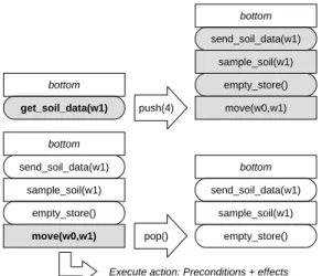
TheStack Machine Simulation(SMS) encoding sim-ulates a stack of tasks which is transformed between computational steps, always checking the task on top of the stack and either pushing its subtasks if it is non-primitive, or executing the corresponding action
get_soil_data(w1) bottom empty_store() send_soil_data(w1) sample_soil(w1) bottom push(4) move(w0,w1) bottom pop() bottom
Execute action: Preconditions + effects
empty_store() send_soil_data(w1) sample_soil(w1) move(w0,w1) empty_store() send_soil_data(w1) sample_soil(w1)
Figure 1: Illustration of the two central transitions between computational steps in the SMS encoding: processing a non-primitive task (top) and a primitive task (bottom).
if it is primitive. This central idea is illustrated in Fig. 1 with a simplified example from the IPC domain “Rover”. Non-primitive tasks have rounded corners and primitive tasks are rectangular. First, the non-primitive task get soil data(w1) is reduced to some valid subtask sequence. In the next step, the primitive taskmove(w0,w1)is processed and removed. Using a stack memory and such transitions, the entire cur-rently considered task hierarchy can be manipulated in a step-by-step manner, eliminating the necessity of linking steps that are further apart.
At the initial step, the firstkpositions of the stack are enforced to contain thekinitial tasks, followed by an explicitbottomsymbol. The goal is defined by the requirement ofbottomto be on top of the stack, or in other words, of the stack being empty.
With this procedure, the initial tasks and their sub-tasks will be sequentially processed and broken down into subtasks until all tasks are removed and only
bot-tomremains. Thereby, the SAT solver decides which
cell of the stack contains which element at which step such that all constraints are satisfied.
The SMS encoding is inherently incremental: To extend an encoding withncomputational steps into an encoding withn+1 computational steps, new clauses are added and the goal assertions (rules 21, 23) are updated. Apart from these simple operations, the pre-vious formula can be reused without any changes.
4.2
Rules of Encoding
All facts specified in the initial state must hold:
^ p∈s0 holds(p,s0)∧ ^ p∈/s0 ¬holds(p,s0) (20)
At the end, all facts from the goal must hold:
^
p∈g
holds(p,sn) (21)
The initial stack contains the initial tasksTand a bot-tomsymbol afterwards. LetT =ht0, . . . ,tj, . . . ,tki:
stackAt(j,tj,s0) (22) stackAt(k+1,bottom,s0)
The stack must be empty in the end:
stackAt(0,bottom,sn) (23)
The execution of an action implies its preconditions to hold:
execute(a,si)⇒
^
p∈pre(a)
holds(p,si) (24)
The execution of an action implies its effects to hold in the next step.
execute(a,si)⇒ ^ p∈add(a) holds(p,si+1)∧ ^ p∈del(a) ¬holds(p,si+1) (25) Facts only change if a supporting action is executed. ¬holds(p,si)∧holds(p,si+1)⇒ _ p∈add(a) execute(a,si) (26) holds(p,si)∧ ¬holds(p,si+1)⇒ _ p∈del(a) execute(a,si)
At each step, all the push(k)andpopoperations are mutually exclusive. Letaandbbe two operations in {push(k)|1≤k≤maxPushes} ∪ {pop}. For each distinct operationaandb, we have:
¬do(a,si)∨ ¬do(b,si) (27)
If nopopoperation is done, then no action is executed, enforced by a virtual actionnoActionwhich does not have any preconditions or effects.
¬do(pop,si)⇒execute(noAction,si) (28)
If an actionais on top of the stack, then it is executed (and only this action); additionally, apopoperation is done.
stackAt(0,a,si)⇒execute(a,si)∧do(pop,si) (29) execute(a,si)⇒stackAt(0,a,si)
If a non-primitive taskt is on top of the stack, then one of its possible reductionsdmust be applied.
stackAt(0,t,si)⇒ _
d∈D(t)
If a non-primitive task t on top of the stack is re-duced by some specific reductiond=ht10, . . . ,tk0i, then apushby the amount of subtasks in the reduction is performed, and all of its preconditions must hold.
stackAt(0,t,si)∧reduc(t,d,si)⇒
⇒do(push(k),si)∧ ^
p∈pre(d)
holds(p,si) (31) The stack content moves according to the performed operation at a given step. Lettbe any task orbottom, andj>0:
do(push(k),si)∧stackAt(j,t,si)⇒
⇒stackAt(j+k−1,t,si+1) (32) do(pop,si)∧stackAt(j,t,si)⇒
⇒stackAt(j−1,t,si+1) (33)
A non-primitive task and a reduction together de-fine the corresponding subtasks as the new stack con-tent at the positions which are freed by the occurring
push operation. Assuming that a reduction of t is
d=ht00, . . . ,tk0−1i: stackAt(0,t,si)∧reduc(t,d,si)⇒ ⇒ k−1 ^ j=0 stackAt(j,t0j,si+1) (34)
4.3
Variants
In addition to this encoding, which we will refer to asSMS-ut(unary tasks) from now on, two additional encodings of SMS have been considered.
The variant SMS-ur(unary reductions) does not
encode tasks, but instead reductions as the content of the stack. This leads to transitional clauses of a differ-ent kind, and the set of variables deciding the chosen reduction are no more necessary.
In the variant SMS-bt (binary tasks), the stack content is encoded not with one variable for each pos-sible task at each position, but instead with one vari-able for each binary digit of a number representing the task at that position. This reduces the total variable re-quirement for the stack content at each cell from
O
(T)to
O
(logT)per computational step, but complicates some transitional clauses.4.4
Complexity
In the following, the asymptotic complexity of clauses and variables of the encoding is discussed. The en-coding variantSMS-utis chosen for this purpose.
As-sume that after n computational steps, a plan π of
length|π| ≤nis found.
The amount of variables is dominated by the en-coding of the stack itself: if a stack of sizeσhas been encoded, then
O
(n·σ·T)variables are used to encode the stack. Additionally, the action executions gener-ateO
(n·A)variables and the state encoding generatesO
(n·F)variables. Moreover,O
(n·r)variables rep-resenting the chosen reduction of the current task areneeded forr=max
|D(t)|
t∈T . This leads to a
total of
O
n·(σT+A+F+r)variables. With some σ∈
O
(n), this measure implies a quadratic termn2T. Regarding the amount of clauses: the classic plan-ning clauses includeO
(n·A) clauses for precondi-tions and effects of acprecondi-tions, andO
(n·F) clausesfor frame axioms (rule 26). To uniquely specify
the content of the stack at each computational step,
O
(n·σ·T·e)transitional clauses (for eachpush(k),1 ≤k≤ e, and for pop) are needed, where e=
max|subtasks(d)|
d∈D(t) .
O
(n·A)clauses linkthe stack operations with the execution of actions. As
eis usually a small constant, a pairwise “at most one action” rule is added by introducing
O
(n·e2)clauses(rule 27). For the actual transitions, each task which can be on top of the stack causes
O
(r·e)clauses; con-sequently,O
(n·T·re)clauses are needed. In total,O
n·(A+F+σTe+e2+Tre)clauses are added. Again assumingσ∈O
(n), the dominating factor be-comesn2Te.5
EXPERIMENTAL EVALUATION
We evaluate the proposed encodings on a set of plan-ning benchmarks. Due to the significant differences regarding recursion in the HTN models (recursion is not supported in (Mali and Kambhampati, 1998)), we cannot directly compare the performances of our dif-ferent encodings. However, the encodings proposed by (Mali and Kambhampati, 1998) have been a start-ing point for the ideas implemented in the GCT en-coding. GCT is then used as baseline in our experi-ments for the SMS encodings that are build on a dif-ferent approach.
A total of 120 instances from six domains have
been considered. The instances have been
gener-ated by using problem generators from the Interna-tional Planning Competition (IPC). All experiments have been conducted on a server with 24 cores of In-tel Xeon CPU E5-2630 clocked at 2.30 GHz and with 264 GB of RAM, running Ubuntu 14.04. Each run has been cut off after five minutes or when its RAM us-age exceeded 12 GB. Glucose (Audemard and Simon, 2009) has been used as the primary SAT solver and as a standalone application to efficiently solve non-incremental formulae produced by GCT. The
applica-Table 1: Run time scores of encodings.
Domain GCT SMS-bt SMS-ut SMS-ur
Barman 0.09 1.90 1.96 4.68 Blocksworld 0.08 9.22 10.94 6.74 Childsnack 0.98 3.90 9.95 4.50 Elevator 4.21 14.86 13.32 10.29 Rover 0.44 6.17 5.40 5.58 Satellite 0.96 7.08 7.17 16.08 Total 6.75 43.13 48.74 47.88 0 8 16 24 32 40 48 56 64
Number of solved instances 0 50 100 150 200 250 300 Time limit / s GCT SMS-bt SMS-ut SMS-ur
Figure 2: Amount of instances solved by each encoding ap-proach relative to the time limit.
tion Incplan (Gocht and Balyo, 2017) has been used as a unified approach to solve the incremental plan-ning problems produced by SMS.
Fig. 2 illustrates the number of instances solved by each competing approach relative to the set time limit. With the GCT encoding, 27 instances have be solved within the maximum time limit. SMS significantly outperformed this baseline: the variantbtsolved 53 instances,utsolved 59 instances, andur solved 63 instances.
A domain-specific comparison of run time perfor-mances is provided in Table 1. For each tested in-stance, a score of 1 is attributed to the competitor with the lowest run timet∗, and a score oft∗/tis attributed to each further competitor with a run timet. Unfin-ished computations lead to a score of 0. For each domain, the scores of all instances are then summed
up. Overall, the variant ur performed best on the
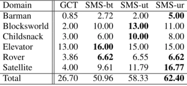
Table 2: Plan length scores of encodings.
Domain GCT SMS-bt SMS-ut SMS-ur
Barman 0.85 2.72 2.00 5.00 Blocksworld 2.00 10.00 13.00 11.00 Childsnack 3.00 6.00 10.00 8.00 Elevator 13.00 16.00 15.00 15.00 Rover 3.86 6.62 6.55 6.62 Satellite 4.00 9.61 11.79 16.77 Total 26.70 50.96 58.33 62.40
Barman and Satellite domains whereas the task-based variantsutandbtgenerally performed better on the Blocksworld and Elevator domains. The binary en-coding variantbtonly lead to small improvements on some domains while significantly worsening the run times on other domains. This result is consistent with the general belief that SAT constraints encoded in a binary manner can actually hinder the propagation of variable assignments and conflicts and, as a result, in-crease the execution time of SAT planning (Ghallab et al., 2004). The length of the plans found with the different encodings are compared in Table 2, with the scores being computed analogously to the run time scores. By design, the GCT encoding generally leads to the shortest possible plan, as the amount of possible primitive actions is increased one by one until a solu-tion is found. The only excepsolu-tion for this is ifnop ac-tions are involved, which do not account for the plan length, but still cause additional solving iterations. Yet, the SMS encoding variants lead to plans which are nearly as short as the plans found with GCT.
6
RELATED WORKS
In his pioneering work, Sacerdoti (Sacerdoti, 1975) proposed a planner called NOAH (Nets of Action Hi-erarchies). The system was built up on a data struc-ture called procedure net. This data structure intro-duced for the first time the concept of tasks network and reduction. These two concepts are today part of all the modern HTN planners. Mali (Mali and Kamb-hampati, 1998; Mali, 2000) proposed to use classi-cal SAT solvers by encoding HTN planning problems into satisfiability problems. Recent and modern HTN planners such as SHOP (Simple Hierarchical Ordered Planner) (Nau et al., 1999; Ramoul et al., 2017) main-tain states during the search process and explore a space of states. Each task network contains a repsentation of the state in addition to the tasks. A re-duction is applicable if and only if some constraints expressed as precondition of the reduction hold in the state. A comprehensive comparison of these different works is given in (Georgievski and Aiello, 2015) and a complexity analysis of HTN planning in (Erol et al., 1994; Alford et al., 2015).
SAT solving has been successfully applied in the classical STRIPS planning context (Fikes and Nils-son, 1971) since the initial proposal (Kautz and Sel-man, 1992; Kautz et al., 1996). As a significant im-provement, more efficient action encodings based on the execution of multiple actions in parallel (as long as some valid ordering on the actions exists) have been proposed (Rintanen et al., 2004; Rintanen et al.,
2006). Recently, incremental SAT solving has been shown to significantly speed up the planning proce-dure of Madagascar (Gocht and Balyo, 2017), based on the observation that reusing conflicts from previ-ous solving attempts can lead to a much faster solving process (Nabeshima et al., 2006).
7
CONCLUSION
In the work at hand, we have presented new efficient approaches of totally ordered HTN planning by mak-ing use of SAT solvers. Previous SAT encodmak-ings for HTN planning problems had many shortcomings re-stricting their practical usage. We proposed two new encodings, GCT and SMS, which mend these short-comings and thus can exploit efficient existing HTN grounding routines. SMS is specifically designed for incremental SAT solving and works reliably on all kinds of special cases which may occur in the consid-ered planning domains. We experimentally evaluated both encodings and showed their practical applicabil-ity by running our planning framework on problem domains from the International Planning Competition (IPC). With the SMS encoding significantly outper-forming GCT regarding overall run times while find-ing plans of comparable length, we have defined a new baseline of SAT planning on totally ordered HTN domains.
In future work, we will investigate alternative SAT encodings based on the general idea of SMS in or-der to further improve the overall performance of the approach. While the SMS encoding works reliably, its performance is limited by the amount of primi-tive actions in the shortest possible plan, and the stack size must be provided as parameter. Enhancements of SMS which function without any external parameters and which require less incremental iterations in order to find a solution may significantly speed up the plan-ning process.
REFERENCES
Alford, R., Bercher, P., and Aha, D. (2015). Tight bounds for HTN planning with task insertion. InProceedings of the International Joint Conference on Artificial In-telligence, pages 1502–1508.
Audemard, G. and Simon, L. (2009). Predicting learnt clauses quality in modern SAT solvers. InIJCAI, vol-ume 9, pages 399–404.
Biere, A. (2013). Lingeling, plingeling and treengeling en-tering the SAT competition 2013.Proceedings of SAT competition, 51.
E´en, N. and S¨orensson, N. (2003a). An extensible SAT-solver. In International conference on theory and applications of satisfiability testing, pages 502–518. Springer.
E´en, N. and S¨orensson, N. (2003b). Temporal induction by incremental SAT solving. Electronic Notes in Theo-retical Computer Science, 89(4):543–560.
Erol, K., Hendler, J., and Nau, D. (1994). UMCP: A sound and complete procedure for hierarchical task-network planning. InProceedings of the Artificial Intelligence Planning Systems, volume 94, pages 249–254. Fikes, R. and Nilsson, N. (1971). STRIPS: A new approach
to the application of theorem proving to problem solv-ing.Artificial Intelligence, 2(3-4):189–208.
Georgievski, I. and Aiello, M. (2015). HTN planning: Overview, comparison, and beyond. Artifical Intel-ligence, 222:124–156.
Ghallab, M., Nau, D., and Traverso, P. (2004). Automated Planning: theory and practice. Elsevier.
Gocht, S. and Balyo, T. (2017). Accelerating SAT based planning with incremental SAT solving. Proceedings of the International Conference on Automated Plan-ning and Scheduling, pages 135–139.
Kautz, H., McAllester, D., and Selman, B. (1996). Encod-ing Plans in Propositional Logic. InProceedings of the International Conference on Knowledge Representa-tion and Reasoning, pages 374–384.
Kautz, H. and Selman, B. (1992). Planning as Satisfiabil-ity. InProceedings of the European Conference on Artificial Intelligence, pages 359–363.
Mali, A. (2000). Enhancing HTN planning as satisfability.
In Artificial Intelligence and Soft Computing, pages
325–333.
Mali, A. and Kambhampati, S. (1998). Encoding HTN planning in propositional logic. In Proceedings In-ternational Conference on Artificial Intelligence Plan-ning and Scheduling, pages 190–198.
Nabeshima, H., Soh, T., Inoue, K., and Iwanuma, K. (2006). Lemma reusing for SAT based planning and schedul-ing. InProceedings of the International Conference on Automated Planning and Scheduling, pages 103– 113.
Nau, D., Cao, Y., Lotem, A., and Munoz-Avila, H. (1999). SHOP: Simple hierarchical ordered planner. In Pro-ceedings of the international joint conference on Arti-ficial intelligence, pages 968–973.
Ramoul, A., Pellier, D., Fiorino, H., and Pesty, S. (2017). Grounding of HTN planning domain. International Journal on Artificial Intelligence Tools, 26(5):1–24. Rintanen, J. (2012). Planning as satisfiability: Heuristics.
Artificial Intelligence Journal, 193:45–86.
Rintanen, J., Heljanko, K., and Niemel¨a, I. (2004). Parallel encodings of classical planning as satisfiability. In Eu-ropean Workshop on Logics in Artificial Intelligence, pages 307–319.
Rintanen, J., Heljanko, K., and Niemel¨a, I. (2006). Planning as satisfiability: parallel plans and algorithms for plan search.Artificial Intelligence, 170(12-13):1031–1080. Sacerdoti, E. (1975). A structure for plans and behavior.