THE VALUE OF TRAVEL TIME AND RELIABILITY-
EMPIRICAL
EVIDENCE FROM KATY FREEWAY
A Thesis by A K M ABIR
Submitted to the Office of Graduate and Professional Studies of Texas A&M University
in partial fulfillment of the requirements for the degree of MASTER OF SCIENCE
Chair of Committee, Mark Burris Committee Members, Yunlong Zhang
Teresa Qu
Head of Department, Robin Autenrieth May 2016
Major Subject: Civil Engineering
ii
ABSTRACT
Travelers place value on both time savings and reliability when choosing a route for a trip. The values of travel time (VOT) have long been an integral part of the appraisal of transport projects. Recently some transport planners have been incorporating the value of travel time reliability (VOR) into transportation project evaluation as well. Whereas VOT measurements have established guidelines, VOR measurement methods are not well established. This research used data that was collected during 2012, 2013, and 2014 that was generated by automated vehicle identification (AVI) sensors from Katy Freeway travelers. Lane choice models were developed to examine the factors
influencing travelers’ lane choice decisions in different traffic conditions and estimate their value of travel time. Models with two independent variables, travel time and toll, resulted in estimated values of travel time from $1.96/hour to $8.06/hour. The estimated value of time was higher for eastbound traffic than westbound traffic. The research could not draw any conclusion on whether the travel time reliability had any impact on
travelers’ lane choice decisions. However, it was observed that a bad trip experience on the general purpose lanes (GPLs) did not have a significant influence on lane choice decision. Furthermore, the percentage of manages lane (ML) trips was higher for the travelers who traveled the whole length of the MLs/GPLs compared to travelers who traveled only a part of the GPLs/MLs. The reason might be that the ends of the MLs provided easier access when compared to the midpoints of the MLs.
iii
DEDICATION
I dedicate this thesis to my parents Mr. Ayub Ali and Mrs. Asma Banu. Everything I did in my life, my sole objective was to make you proud.
iv knowledge to complete this work.
Many individuals need to be acknowledged for their continuous and sincere support during the research process. First, I would like to thank my supervisor Dr. Mark Burris, for his time, generous guidance, attention, and unwavering encouragement throughout the whole research period. I also wish to extend my gratitude to Dr. Yunlong Zhang and Dr. Teresa Qu for their kind encouragement and guidance. The thesis work was a great learning process for me and I had the privilege to work under these knowledgeable and experienced mentors.
Thank you my dear wife, Sirajum Munira, for being a wonderful support in every way. I should admit that without her inspiration and help, I could not finish my thesis. I would like to express my sincere appreciation to my friends and colleagues, Sunghoon Lee and Santosh Rao, who extended their support during this research. The hard period of work seemed easy and less stressful because of their company.
The thesis was, in part, an outcome of the research project titled “Traveler’s value of time and reliability as measured on Katy freeway” which was supported with funds from the Texas A&M Transportation Institute’s Policy Research Center. Again, I would like to thank Dr. Mark Burris for his insights and guidance on this project. I also appreciate the sharing of data by TxDOT and Harris County Toll Road Authority (HCTRA) without which none of this effort would have been possible.
v GPLs General Purpose Lanes
GPS Global Positioning Systems HOV High Occupancy Vehicle HOT High Occupancy/Toll
HCTRA Harris County Toll Road Authority MLs Managed Lanes
RP Revealed Preference RR Reliability Ratio SP Stated Preference
TxDOT Texas Department of Transportation
USDOT United States Department of Transportation VOR Value of Travel Time Reliability
vi ABSTRACT... ii DEDICATION ... iii ACKNOWLEDGEMENTS ... iv NOMENCLATURE ... v TABLE OF CONTENTS ... vi
LIST OF TABLES ... viii
LIST OF FIGURES ... x
1. INTRODUCTION ... 1
1.1 Research Problem and Objective ... 4
2. LITERATURE REVIEW ... 5
2.1 The Value of Travel Time ... 5
2.2 The Value of Travel Time Reliability ... 10
2.3 Mathematical Framework to Estimate VOT and VOR ... 15
2.4 Stated Preference Studies ... 18
2.5 Revealed Preference Studies ... 21
3. DATA………26 3.1 Transponder Data ... 26 3.2 Toll Data ... 27 4. METHODOLOGY ... 30 5. DATA ANALYSIS... 34 5.1 Processing of Data ... 34
5.1.1 Cleaning, Merging and Randomization of Data ... 34
5.1.2 Exclusion of Specific Entries ... 34
vii
5.2 Overview of Paid ML Trips ... 41
5.2.1 Frequency of Paid ML Use ... 46
5.3 VOT and VOR Analysis ... 48
5.3.1 Value of Time Estimation Using Basic Models ... 48
5.3.2 Basic VOT and VOR Models by Month ... 51
5.3.3 VOT and VOR Models without Uneconomical Trips and Non-switching Travelers ... 54
5.4 The Impact of a Bad Trip Experience on Lane Choice ... 59 5.5 The Impact of Number of Trips on Lane Choice ... 63
5.6 The Impact of the Length Traveled of MLs/GPLs Section on Lane Choice ... 70
6. SUMMARY AND CONCLUSIONS ... 78
6.1 Limitations ... 84
REFERENCES ... 85 APPENDIX...88
viii
Table 1 Empirical estimates of VOT ... 7
Table 2 Commonly used reliability measures ... 11
Table 3 Empirical estimates of VOR ... 13
Table 4 Katy managed lane toll rates ... 29
Table 5 Decrease in the number of trips based on time limit between detection ... 36
Table 6 Average travel speeds by period ... 37
Table 7 Number of alternate trips by type ... 39
Table 8 Percentage of alternate trips by type ... 39
Table 9 Number of recorded trips ... 42
Table 10 Paid trips on managed lane ... 42
Table 11 Travel time saving on the managed lane ... 44
Table 12 Basic VOT results by month ... 49
Table 13 Value of travel time ($/hour) by time period ... 50
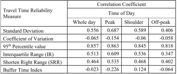
Table 14 Correlation between travel time and travel time reliability... 51
Table 15 Model results summary ... 53
Table 16 Model results summary for the travelers who had at least one trip on each lane ... 56
Table 17 Number of cases where anticipated result was seen ... 57
Table 18 Number of cases where anticipated result was seen (for travelers who had at least one trip on each lane) ... 58
Table 19 Logit models with time and toll and bad trip experience as independent variable ... 61
ix
Table 21 Traveler’s total trips during the previous 30 days and current lane
choice decision ... 64
Table 22 Traveler’s MLs trips during the previous 30 days and current lane choice decision ... 65
Table 23 Model results including the number of trips during the previous 30 days and the number of ML trips during the previous 30 days variables ... 66
Table 24 Traveler’s total trips during the previous 30 days and current lane choice decision (for travelers who had at least one trip on each lane) ... 68
Table 25 Traveler’s MLs trips during the previous 30 days and current lane choice decision (for travelers who had at least one trip on each lane) ... 68
Table 26 Model results including the number of trips during the previous 30 days and the number of ML trips during the previous 30 days variables (for travelers who had at least one trip on each lane) ... 69
Table 27 ML and GPL trips by time of day and trip category ... 70
Table 28 Basic VOT results by month (category 1 traffic) ... 74
Table 29 Basic VOT results by month (category 2 traffic) ... 75
Table 30 Model result summary for category 1 traffic ... 76
x
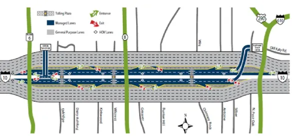
Figure 1 Katy Freeway (HCTRA,2009) ... 27
Figure 2 AVI sensors along Katy Freeway ... 28
Figure 3 Total toll paid on the managed lanes ... 43
Figure 4 Travel time saved (minutes) on the managed lanes ... 43
Figure 5 Toll paid divided by time saved ... 45
Figure 6 Number of trips by length ... 45
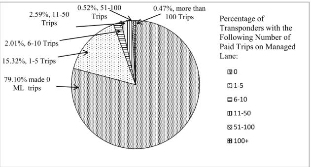
Figure 7 ML trips made by all transponders recorded on the freeway... 47
Figure 8 Percentage of trips that were paid ML trips by transponder ... 47
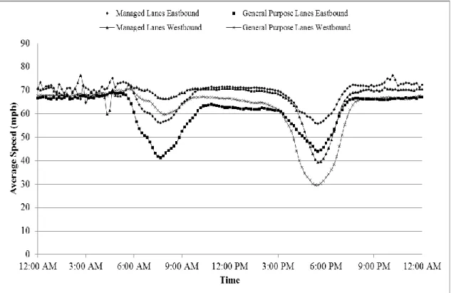
Figure 9 Average travel speed distribution ... 60
Figure 10 Traffic on the IH-10 Katy freeway viewed facing west near Loop 610 on Thursday, April 11, 2013, in Houston(Houston Chronicle, 2014) ... 73
1
1.
INTRODUCTION
Investment in improved transport infrastructure typically leads to a reduction in traveler’s travel time and an increase in travel time reliability. The value of travel time (VOT) has long been an integral part in the appraisal of transport projects. In the case of travel time, transportation planners, engineers and economists try to estimate travelers’ value of time (VOT). Value of time is the equivalent amount of money a traveler would pay for a reduction in the amount of time to complete a trip. For example: if a traveler would pay one dollar to reduce their travel time by six minutes then they would have a VOT of $10/hour.
Similarly, travelers also value trips where they can expect to arrive on time, which refers to the reliability of travel time. According to the Federal Highway Administration (FHWA), travel time reliability is the consistency or dependability of travel times, as measured from day-to-day and/or across different times of the day. Quantitatively, the economic worth of travel time variation is referred to as the value of reliability (VOR). VOR is equivalent to the amount of money a traveler would be willing to pay to reduce the variation in their expected travel time.
In recent years, agencies have recognized the importance of improved travel time reliability in the evaluation of transportation projects. Many countries, such as New Zealand, Australia, and the Netherlands, have published guidelines to incorporate travel time reliability into their economic appraisal of transportation projects. In the USA, the federal government provided funds for extensive research on travel time reliability. The
2
second Strategic Highway Research Program (SHRP 2) was authorized by the United States congress to conduct research projects that focused, in part, on reliability-related issues.
In the last 40 years, the VOT has been comprehensively studied and most agencies have a guideline to estimate the VOT. On the other hand, methods of estimating the value of reliability are still a topic of debate. Different studies have used different reliability measures which lead to inconsistency among the obtained VORs. A majority of the researchers have used stated preference survey data to estimate VOR and the estimated values varied significantly based on survey design, location, sample size and methods of measuring reliability. Carrion and Levinson (2012) examined the
shortcomings of the stated preference studies suggesting that most of the researchers did not focus on survey data validation, and that it is difficult to be certain about which estimates are more plausible than others. On the contrary, very few studies have used revealed preference (RP) data to estimate VOT and VOR. One of the main reasons is that a proper experimental design for a revealed preference study is difficult when compared to that of stated preference study.
One important issue to estimate VOR is determining how travelers perceive reliability. Several reliability measures such as standard deviation, 95th percentile of
travel time, shorten right range, and buffer time index have been used in the literature. But a traveler may perceive reliability in his/her personal way which may not be well represented by the commonly used reliability measures. The travelers’ familiarity with a
3
route might have an influence on his/her perception of reliability. For example, a traveler might consider his/her previous 5 trips when deciding whether a route is reliable or not. In addition, to a particular traveler, reliability of a route may vary depending on the day of week and time of day.
To address the limitations of the previous studies on VOT and VOR, Alemazkoor et al. (2014) used data from Katy Freeway, Houston. Here travelers choose between more reliable Managed Lanes (MLs) and toll free General Purpose Lane (GPLs). The dataset consisted of records generated from automated vehicle identification (AVI) sensors placed at regular intervals along the freeway. The study indicated that travelers on the Katy freeway might not consider travel time reliability while making lane choice decisions or the reliability measures used in the study could not represent the reliability perception of the travelers. The study indicated that one potential reason why they could not get expected results as they have used only one month of data with no variation in toll schedule. Therefore, a more comprehensive study with data, collected for longer period with a varying toll schedule, may help to better understand the travelers’ perception of reliability.
This study will use data generated from automated vehicle identification sensors from Katy Freeway travelers collected during 2012, 2013, and 2014. These data include travel times on all lanes and tolls paid to use the Katy Freeway Managed Lanes .Thus it is possible to know how much travelers spent to use the MLs , how much travel time they saved (if any) ,and how much more reliable the MLs were (if at all) as compared to
4
the general purpose freeway lanes . In addition, the toll schedule has been updated twice during these three years. This provides additional variation in the toll (data) variable which generally leads to improved model prediction ability. Moreover, as the dataset allowed tracking all trips for a traveler on the Katy freeway, it provides an opportunity to see how previous trip experience and familiarity with the freeway impacted lane choice. 1.1 Research Problem and Objective
This research examines the impact of different factors, such as tolls, travel time saving, travel time reliability and familiarity on the traveler’s choice between general purpose lanes and managed lanes. The study also compares the effectiveness of different reliability measures. This research investigates the effect of previous bad trip experience on lane choice decision models.
The main objectives of this study are:
1. To examine the factors that influence travelers’ lane choice decision in different traffic conditions
2. To better understand how reliability impacts lane choice decision 3. To explore the influence of travelers’ previous experience (based on
number) of trips on lane choice decision
4. To estimate traveler willingness to pay for travel time saving and improved travel time reliability
5
2.
LITERATURE REVIEW
2.1 The Value of Travel Time
The value of travel time (VOT) is the measure of travelers’ willingness to pay for a reduction in their travel time. Existing literature on the VOT is very comprehensive and well developed. The first analysis of VOT was a 1925 Bureau of Public Roads report (U.S. Bureau of Public Roads and the Cook County Highway Department, 1925) which estimated VOT to be $3 per hour (in 1925 dollars, approximately $41 per hour when increased by inflation to 2015 dollars). Studies between 1925 and the 1970s generally used one of two methods to estimate VOT: (1) the VOT was assumed to be equal to the travelers wage rate or (2) how much travelers would be willing to pay to use a faster mode of travel. For example, how much more would a traveler be willing to pay to travel by car than by bus? Since then, most studies have used stated preference survey data to estimate value of time. These stated preference studies generally asked travelers to choose between modes and developed logit equations to predict mode choice. VOT was estimated based on the coefficients in those equations.
Concas and Kolpakov (2009) summarized many VOT studies (see Table 1). They found that many analyses had found a strong relationship between the traveler’s hourly wage rate and their VOT. The estimated VOTs ranged from 20% to 100% of the traveler’s hourly wage rate and most of the literature suggested that the VOT should be around 50% of hourly the wage rate for personal trips. This is similar to US DOT guidance (USDOT, 2003). Brownstone and Small (2005) conducted a study on SR-91
6
and I-15 in Southern California and estimated the VOT for personal trips to range from $20/hour to $40/hour. For commercial trips, VOT can be higher than the hourly wage rate. Waters (1992) found that travelers valued their time for commercial travel could be as high as 1.7 times their average wage rate.
The literature shows that the value of travel time depends on various factors: type of travel, personal characteristics (age and sex) of traveler, transportation mode (bus, car, bicycle or walk), and travel condition (level of service). Disrepair (1971) mentioned that time spent in any activity is a matter of choice as well as a matter of necessity. Thus, for an individual the value of travel time would depend on trip purpose. Many agencies have recommended using different values of time for different types of travel. The U.S. DOT (2003) recommended values of time were $10.60/hour for commuter travel and
$21.46/hour for business travel. In New Zealand the recommended values of travel time were NZ$7.8 for commuter travel and NZ$23.85/hour for business travel. Cal fee and Winston (1998) gave an explanation about the lower estimation of commuters’ value of travel time. They collected data from the National Family Opinion Survey which covered commuters from major U.S. metropolitan cities. They found that commuters’ average value of travel time saving ranged from 14% to 26% of the gross wage. According to Calfee and Winston (1998), the value of travel time was insensitive to travel condition; commuters are able to adjust to congestion through their modal and departure time choice, as well as the choice of residential and workplace location (Concas and Kolpakov, 2009).
7
Several studies have tried to estimate the value of time on managed lanes. Using stated preference data, a study for the Georgia Department of Transportation (GDOT) found that the estimated value of time for autos would range from $7/ hour to $15/ hour, while a commercial vehicles trip can have a value of time of $23/hour (HNTB ,2010). Another study for the Florida Department of Transportation (FDOT) estimated the value of travel time for autos to be in range of $2.27/hour to $79.32/hour (Perk et al., 2011). A study on the Katy Freeway by Devarasetty et al. (2012) using stated preference survey data (Db-efficient design) estimated the value of travel time to be $22/passenger car hour.
Table 1 Empirical estimates of VOT
Study Data Used VOT Estimate
U.S. Bureau of Public
Roads (1925) Survey of highway transportation $3.00 Beesley(1965) Data from the survey of
government employees in London, UK
31%‐50% of wage rate
Lisco (1967) Survey of multiple route choice models
60% of gross wage (on average)
Small (1992) Values derived from multiple mode choice transportation models
20% to 100% of gross wage; 50% ‐ reasonable average
8 Table 1 Continued
Study Data Used VOT Estimate
Waters (1996) Travel data from 15
commuting studies in North America
40%‐50% of after tax wage rate (mean: 59% of after tax wage rate; median: 42% of wage rate)
Small and Yan(2001) Data on commute travelers on SR‐ 91 in California
Average VOT was $22.87/hour, or 72% of sample wage rate Brownstone and Small
(2005) Travel data from ETC facilities in HOT lanes on SR‐91 and I‐15 in Southern California
VOT saved on the morning
commute: $20‐$40 per hour, or 50%‐90% of average wage rate in the sample
USDOT (Ayala, 2014) Estimates are based on
multiple sources of data 50%rate ‐120% of the wage depending on type of travel
(personal vs. business); 50% of wage rate for personal local travel and 100% of wage rate for commercial local travel USDOT (Ayala, 2014) Compilation of many
sources
Local travel, all purposes is $12.80 in 2012 dollars.
9
The value of travel time depends on various factors such as the type of travel, the characteristics of the traveler (for example, age and gender), transportation mode (for example, bus, car, or walk), travel condition, time of the year, or week, or day, location, and trip purpose. Many agencies have recommended using different values of time for different types of travel. The U.S. DOT recommended values of time were $10.60/hour for commuter travel and $21.46/hour for business travel. The latest update to these guidelines (USDOT, 2014) suggested values of time of $12.50 in 2009 dollars for all purposes of travel combined.
Most of the studies in the last 40 years have used stated preference (SP) surveys to estimate VOT. As mentioned by Carrion and Levinson (2012), early studies were based on questions that asked travelers to choose between hypothetical travel alternatives. For example, would they choose option 1 which takes 10 minutes and requires a $2 toll, or option 2 which takes 15 minutes but has no toll.
Carrion and Levinson (2012) found that in some cases researchers who conducted stated preference studies presented survey data in a format that reflected the researchers’ intended outcome. Literature suggests that most researchers did not validate survey data, and that estimates were hard to evaluate for plausibility. Very few revealed preference studies were found that could be used to validate the outcome from stated preference studies.
Many countries have incorporated VOT into their economic evaluation of
10
based on a national survey conducted in 1998. Since then the values have been adjusted every year for inflation and for real income changes. In 2010, the recommended values of travel time were €9.92/hour for commuter trip and €34.36/hour for business trip (approximately $9/hour and $31/hour in US dollars). New Zealand’s Economic Evaluation Manual provides guidelines to incorporate VOT into economic evaluations for surface transportation projects (such as highway, transit and rail). New Zealand suggested different VOT ranges based on types of vehicles, roadway network and day of week. In 2013, the value of travel time ranged from NZ$14.96/hour to NZ$25.84/hour (approximately $22/hour and $38/hour in US dollars).
2.2 The Value of Travel Time Reliability
Although the concept of travel time reliability is not new, valuing travel time reliability is not well established. The value of reliability (VOR) is equivalent to the amount of money a traveler would be willing to pay to reduce the variation in their expected travel time. Researchers have attempted to quantify VOR and the estimated values are a subject of continuous debate (Carrion and Levinson, 2012). A main reason for the discrepancy is due to researchers using different approaches to measuring travel time reliability. Definitions of commonly used reliability measures are summarized in Table 2.
11 Table 2 Commonly used reliability measures
Reliability Performance
Metric Definition
Buffer Index (BI) The difference between the 95th percentile travel time and the average (or median) travel time, divided by the average (or median) travel time
Failure/On‐Time Measures Percent of trips with travel times less than 1.1 × Median Travel Time or 1.25 × Median Travel Time Percent of trips with space mean speed less than 50 mph; 45 mph; or 30 mph
80th Percentile Travel
Time Index 80th percentile travel time divided by the freetravel time ‐flow Planning Time Index 95th percentile travel time divided by the free‐flow
travel time
Skew Statistic The 90th percentile travel time minus the median all divided by the median minus the 10th percentile Misery Index (Modified) The average of the highest 5 percent of travel times
divided by the free‐flow travel time Standard Deviation of
Travel Time or Travel Rate Root‐mean‐square deviation of travel time
√1
𝑁∑(𝑥𝑖 − 𝜇)2 𝑁
𝑖=1
Where,
xi = Travel time of trip i
μ = Average travel time
N= Total number of observation Shorten Right Range
(SRR) The difference between 90th percentile travel time and median travel time Interquartile Range (IR) The difference between 75th percentile and 25th
percentile travel time
12
Early studies used standard deviation as the measure of travel time reliability. More recent studies have used the difference between two percentile values within a travel time distribution (95th and 50th, 90th and 50th, or 80th and 50th) to estimate reliability.
Tilahun and Levinson (2010) used three measures to estimate VOR, which were: (1) Probability of early or late arrival compared to usual travel time,
(2) Difference between maximum travel time and median (the median travel time is the travel time where half of travelers were slower and half were faster), and
(3) Standard deviation.
Their findings suggested that all three approaches yielded a similar output. Van Lint et al. (2008) found that using different measures of reliability would provide inconsistent results. They compared results from using the standard deviation, coefficient of variation, buffer index and misery index. Alemazkoor et al. (2014) examined how well different value of reliability measures matched actual traveler behavior data from Katy Freeway. Their results were inconclusive and possibly
indicated that many travelers did not consider reliability, or it was far less important than other variables, when making their travel decisions.
The National Cooperative Highway Research Program (NCHRP Report-399, 1998) suggested using the standard deviation as a measure of travel time reliability. Many countries including New Zealand, Australia, the Netherlands, and the United Kingdom prefer using standard deviation as measure of travel time reliability for passenger travel.
13 Table 3 Empirical estimates of VOR
Study Data Used VOR Estimate Definition of
Reliability Black and
Towriss, (1993)
Data from SP survey of travelers in
London
0.55‐0.70 of travel time Measured as standard deviation of travel time Small, Noland, Chu and Lewis (1999) SP survey of travelers in SR‐91 corridor in Orange and Riverside counties in Southern California, conducted in 1995 Average of 2.37 of travel time for median income and all trips ($12.60/hour)
Greater than 3 times of travel time for work trips and higher income
Reliability is measured by standard deviation of travel time Lam and Small (2001)
Travel time data from loop detector from SR-91 and RP data through mail
$15.12/hour for men and $31.91/hour for women
standard deviation, and difference between 90th
percentile and median travel time Brownstone
and Small (2003)
Travel data from ETC facilities in HOT lanes on SR‐91 and I‐15 in Southern California, 1996‐ 2000 95%‐140% of the median travel time
Difference between 90th and 50th percentile travel time Tseng, Ubbels and Verhoef (2005)
Data from surveying Dutch commuters, 2004 VOR is valued at ½ of the VOT (5.3 Euros/hour, or $6.41/hour) Difference between
early /late arrival time and preferred arrival time. Early and late arrivals are modeled separately
14 Table 3 Continued
Study Data Used VOR Estimate Definition of
Reliability Small,
Winston and Yan
(2005)
Travel data from SR‐91 in greater Los Angeles area, 1999‐
2000
VOR estimated at $19.56/hour, or 85% of average wage rate
Difference between 75th and 25th percentile travel time Tilahun and Levinson (2007) Data from a SP route choice survey of University of Minnesota employees, Minneapolis/St. Paul, MN
Equivalent to VOT Difference between
actual late arrival and usual (mode) travel time Devarasetty et al. (2012)
Internet based stated preference survey $28/hour Coefficient of variability Carrion and Levinson (2012)
GPS based RP data $0.32/hour-$3.84/hour for men and
$4.9/hour-$8.6/hour for women
Standard deviation
Sources: Many are from Concas and Kolpakov (2009)
The literature suggests that studies have used different reliability measures to estimate value of reliability. But a majority of the studies used stated preference data to estimate value of reliability (See Table 3). As mentioned earlier that the estimated value of reliability is not consistent. A study on the SR-91 in greater Los Angeles area by small et al. (2005) estimated the value of reliability to be 19.56/hour, or 85% of average
15
wage rate of the sample. A study by Tilahun and Levinson (2007) found that the value of travel reliability would be equivalent to the value of travel time. Carrion and Levinson (2012) using GPS and RP data found that the value of reliability ranged from $0.32/hour to $8.6/hour. As the studies differed in data collection methods, location, sample size and measurement of reliability, it is not possible to decide which estimation is better than others.
2.3 Mathematical Framework to Estimate VOT and VOR
So far, three different frameworks have been used to mathematically describe travel time and reliability: (1) centrality dispersion or mean variance, (2) scheduling delay, and (3) mean lateness.
Centrality Dispersion, introduced by Jackson and Jucker (1982), is based on the concept where travelers want to minimize their disutility from travel time and travel time unreliability. The utility function used in this method is estimated using discrete choice methods. The utility or disutility function is formulated as Equation 1:
𝑈(𝑝) = 𝜆1𝑘𝜇 𝑇𝑝+ 𝜆2𝑘𝜎𝑇𝑝 + 𝜆3𝑘𝐶𝑝 (1)
Where,µ is the mean travel time , σ is the standard deviation of the travel time distribution ,Cp is the cost associated with travel and λ is the coefficient which indicate the degree to which the independent variable affects traveler k’s utility on route p. The value of time (VOT) and the value of reliability (VOR) can be obtained by computing marginal rate of substitution. These are defined as,
16 𝑉𝑂𝑇 =𝛿𝑈⁄𝛿𝜇𝑇 𝛿𝑈 𝛿𝐶 ⁄ (2) 𝑉𝑂𝑅 =𝛿𝑈⁄𝛿𝜎𝑇 𝛿𝑈 𝛿𝐶 ⁄ (3)
Small(1982) developed scheduling delay approach considering that travelers utility was influenced by departure time and workplace constraints. According to the
scheduling delay approach, utility/disutility is involved with early arrival as well as late arrival.
U(td)=β1 T+β2 SDE+β3 SDL+β4 DL+ β5 C (4)
Equation 4 represents the utility function for departure time (td). Here, utility is
described as a function of travel time (T), schedule delay early (SDE), schedule delay late (SDL), a dummy variable (DL) which depends on the value of SDL, and a cost variable (C). Here, β is the coefficient which indicates the degree to which the independent variable affects traveler’s utility. The utility function can be used to
estimate the value of time, the value of scheduling delays early (VSDE) and the value of scheduling delays late (VSDL).
𝑉𝑂𝑇 =𝛿𝑈⁄𝛿𝑇 𝛿𝑈 𝛿𝐶 ⁄ (5) 𝑉𝑆𝐷𝐸 =𝛿𝑈⁄𝛿𝑆𝐷𝐸 𝛿𝑈 𝛿𝐶 ⁄ (6) 𝑉𝑆𝐷𝐿 =𝛿𝑈⁄𝛿𝑆𝐷𝐿 𝛿𝑈 𝛿𝐶 ⁄ (7)
17
The Association of Train Operating Companies (ATOC) introduced the mean lateness approach and it has become the standard for reliability analysis for rails travel in the United Kingdom. This approach used schedule journey time (SchedT) and mean lateness (L) to express the utility function. Here, β is the coefficient which indicates the degree to which the independent variable affects traveler’s utility. If a cost variable is added in the utility function, value of lateness can be measured.
U(td)=β1(SchedT)+β2L+ β3C (8)
𝑉𝑂𝐿 =𝛿𝑈⁄𝛿𝐿 𝛿𝑈
𝛿𝐶
⁄ (9)
Black and Towriss (1993) introduced a term reliability ratio (RR) expressed as ratio of VOR and VOT. Many countries are using reliability ratio to predict VOR (Nevers et al., 2013), which can be further implemented in economic evaluation for transportation projects.
𝑅𝑅 =𝑉𝑂𝑅𝑉𝑂𝑇 (10)
The data used in this study contains the information not only about travelers’ lane choice decision but also information about how much travel time they saved (if any) , how much toll they had to pay on MLs(if any) ,and how much more reliable the MLs were (if at all). These attributes (travel time, reliability and tolls) can be easily
18 2.4 Stated Preference Studies
The literature indicates that most of the studies used stated preference (SP) surveys to estimate the value of travel time and the value of reliability. As mentioned by Carrion and Levinson (2012), early studies were based on paired comparison questions of hypothetical route alternatives. In a question, each hypothetical route had a “usual” travel time. Also, a delay component was assigned to one of the routes, usually the route with the shortest travel time. Jackson and Jucker (1982) used this kind of stated
preference technique to gather data. In their study, in a pair, one alternative had a usual travel time (15, 20, 50 minutes etc.) which was higher than other alternative’s travel time (10, 20, 30 minutes etc.). The later alternative corresponded with a range of delay (5-20, 10-40, 5-50 minutes etc.) and a delay occurrence frequency (once a week, twice a week, once a month etc.). The study found that the variability of travel time had a significant impact on route choice and the impact varies across individual. They also found that the mean variance approach provided extremely accurate prediction.
Black and Towriss (1993) used an approach that presented data in a different way. In their approach, each route had same mean travel time but different travel cost. For presenting variability they assigned several possible travel times to each route. The survey respondents chose one route from the two alternatives. Black and Towriss (1993) used the mean-variance approach to analyze the data. They found that travel time
reliability was a significant factor, though the magnitude was less than the magnitude of mean travel time. Depending on their models the reliability ratio ranged from 0.55 to
19
0.7. Small et al. (1999) used Black and Towriss (1993)’s question format with some modifications. In their survey design, each alternative consisted of a mean travel time, a distribution of five arrival times with respect to an implied preferred time, and a travel cost. Using the survey data, Small et al.(1999) estimated mean-variance models, scheduling models and a econometric model that combined both of the approaches ( mean-variance and scheduling). They found that the combined model lead to an estimate of the travel time reliability measure that was not statistically significant. It should be noted that their study found a reliability ratio of 3.22 which was much higher than the reliability ratios found in other contemporary studies. This indicated that the design of survey might have significant effect on estimation of value of travel time and value of reliability.
Many researchers have tried alternative presentations of survey data to estimate travelers’ value of reliability. Hensher (2001) used bar diagrams with minute values for four components of the total travel time: free flow, slow down, stop/start and
uncertainty. A travel cost component was associated with each alternative which allowed them to calculate tradeoffs between cost and the distinct component of travel time. As mentioned by Carrion and Levinson (2012), Hensher (2001) was focused on
investigating the value that travelers assign to the distinct components of total travel time rather than travel time reliability. Cook et al. (1999) and Bates et al. (2001) proposed a design, for the presentation of variability, which consisted of representation of arrival time with respect to given preferred arrival time. They also included survey phases to familiarize the responders to their data presentation. Copley et al. (2002) used a
20
qualitative approach to study different presentations of travel time variability: linear arrangement of possible travel times, circular arrangements of possible travel times, and histogram representation of possible travel times. They found that the histogram
presentation was easier to understand and it can present large volume of information. Tseng et al. (2009) used face to face interviews to investigate the most preferable way to represent survey data. Tseng et al. (2009) asked the responders about the preferences with regards to the format. They also asked questions that tested respondents’ choice consistency and logic of perception with regards to reliability presented in the questionnaires. The study found that respondents could easily understand if data was presented as Small et al. (1999)’s format. The values of time and the values of reliability observed in the stated preference studies are not consistent. Depending on the survey design and selection of the respondents the estimated values differed significantly.
Devarasetty et al. (2012) used survey data and actual usage data from Katy Freeway travelers to estimate their value of travel time reliability. During the survey, approximately half of the respondents received questions in pictorial format and other half received questions in text-only format. The respondents were given four options for each question: drive alone on general purpose lane, drive alone on toll lanes, carpool on general purpose lanes, and carpool on toll lanes. The study found that the survey format had no significant effect on the result. The research outcome showed that the combined estimate of the VOT and VOR base on stated preference data to be $50/hour, which was almost equal to the estimated VOT of $51/hour estimated from actual usage data.
21
In summary, it can be said that stated preference surveys were widely used to estimate value of travel time and value of reliability. One important point indicated by Carrion and Levinson (2012) was that, in stated preference studies, researchers might present the survey data in such ways that reflect their own intended outcome. The literature suggests that most of the researchers did not focus on survey data validation, and that it is difficult to be certain about which estimates are more plausible than others. There are very few revealed preference studies which can be used to validate the stated preference studies’ outcome. The revealed preference studies will be discussed in the following section.
2.5 Revealed Preference Studies
In comparison to the large number of stated preference studies, there are very few studies that have used revealed preference (RP) data to estimate value of time and value of reliability. One of the main reasons is that a proper experimental design for revealed preference is difficult when compared to that of stated preference experiment design. Lam and Small(2001) used loop detector data and survey data to estimate value of reliability for the travelers on State Route(SR) 91 in Orange County, California. They conducted a mail survey among the travelers (533 respondents) to gather information about the travelers’ most recent trips. They also estimated the average travel time within the same time of day using loop detector data. One of the limitations of the study was the loop detector had been collected one year prior to the mail survey. The researchers then adjusted the travel times using data factor of 1.37 which implied that on that particular
22
route in one year the travel time had increased by 37%. In addition, the travel times obtained using loop detector data were averaged over 15 minutes. Therefore, calculated travel times may not represent the actual travel time of the travelers. The study found that if the travel time reliability is expressed as the difference between 90th percentile
and the median of travel time, it provides the best fit model. According to the model, the value of reliability was $15.12/hour for men and $31.91/hour for women.
Small et al. (2005) used a combination of RP and SP data of travelers on SR 91 to estimate their VOR. Telephone interviews and mail-back surveys were conducted to collect the data. Though there were 522 participants in RP survey and 633 participants in SP survey, only 55 participants were found who participated in both surveys. Therefore, a combination of both datasets might cause errors in the study. Moreover, the researchers concluded that the RP data can never be representative of the real world scenario
because there is a chance of perception error during the survey. The study estimated the median VOR of $19.56/hour.
Carrion and Levinson (2013) designed a GPS-based experiment to estimate the VOR of travelers on I-394 in Minnesota. The researchers used a web based application to recruit 18 regular commuters who had been using the study route. Relevant personal information was available from their application. The cars of the respondents were equipped with GPS devices to track their actual travel. For the first two weeks, the commuters traveled on each of the three alternatives (HOT lanes, general purpose lanes [GPLs] and adjacent signalized arterials) separately. During those two weeks they better
23
understood the travel time and reliability on each route. After that they were instructed to travel on their preferred route. The design was able to depict a real world scenario, though the sample size was very small (18 respondents) to draw any unbiased conclusion. The study produced wide range of VOR depending on the travel time reliability definition.
Alemazkoor et al. (2014) used data from Katy Freeway, Houston, where travelers choose between Managed Lanes (MLs) and General Purpose Lane (GPLs). The dataset generated from automated vehicle identification (AVI) sensors placed at regular
intervals along the freeway. They have attempted to find the best measure of reliability from standard deviation, 95th percentile value, coefficient of variation, buffer time index,
shorten right range, interquartile range, travel time index, and misery index. But many of the reliability measures lead to counter-intuitive results. Depending on the measures of reliability and traffic characteristics their estimated VOR varied from $1.98/hour to $24/hour. The study indicated that travelers on the Katy freeway might not consider travel time reliability when making lane choice decisions or the reliability measures used in the study could not represent the reliability perception of the travelers. The study indicated that one potential reason why they could not get expected results as they have used only one month of data with lack of variation in toll schedule. It should be noted that the current study will use similar data to what was used by Alemazkoor et al. (2014), but three years of travel data will be used instead of one month of data.
24
The revealed preference studies showed that the routes along high occupancy toll lanes are the most popular location for experiments. In general, travelers have two route alternatives: high occupancy toll lanes and parallel untolled lanes. In some of the
revealed preference studies, the researchers approximated the travel time of the traveler using loop detector data or in field measurements (driving in similar traffic condition). There is a high possibility that travel data is different from the actual scenario. Using GPS device in respondents’ car is an effective way to get actual travel time data but this method is costly and thus difficult to get a large enough sample to be representative of actual travelers.
In summary, the review of existing literature highlighted that comprehensive studies are available assessing VOT and most agencies have guidelines to estimate VOT to use in transport project appraisals. On the other hand, methods of estimating VOR are still a topic of debate. Most studies have used SP survey data to estimate VOT and VOR as a proper experiment design for RP data is complicated and generally not available. Moreover, estimated VOR vary significantly across studies based on estimation
methodology and reliability measures used. As most of the researchers did not focus on survey data validation, it is difficult predict which estimates are more plausible than others. A few studies (Lam an Small, 2001, small et al. ,2005, and Carrion and Levinson, 2013)have used RP data to estimate VOR, but they either had a sample size too small to provide unbiased results or had to make some assumptions which might have an effect on the estimated value. The study by Alemazkoor et al. (2014) used one month of actual data and indicated that travelers might not consider travel time reliability while making
25
lane choice decisions or the reliability measures used in the study could not represent the reliability perception of the travelers. Therefore, a more comprehensive study with RP data, collected for longer period with a varying toll schedule, may help to better understand the travelers’ actual value of reliability and travel time saving.
26
3.
DATA
3.1 Transponder Data
TxDOT collects transponder data using automated vehicle identification (AVI) sensors located on both the MLs and GPLs along the Katy Freeway. Figure 2 shows the location of the sensors where each number indicates a specific sensor. When a sensor detects a vehicle with transponder, it inserts a new record into a database where the sensor ID, detected vehicle’s transponder ID, and detection time are recorded. All vehicles that pay a toll on the MLs are required to use a transponder. Many other vehicles traveling on GPLs also have transponders. The AVI data obtained from TxDOT contains all sensor detection records from most of 2012, 2013 and 2014. The data were obtained from TxDOT in October 2014 so the data only include up until September 2014. Also, some days at the end of December 2012 were missing and therefore, December 2012 was not included in the analysis.
The Harris County Toll Road Authority (HCTRA) operates AVI sensors along the MLs at the three toll plaza locations (see Figure 2 for HCTRA sensors). The data obtained from HCTRA included the unique transponder ID, toll plaza ID, and date and time of record for each vehicle traveling within the MLs for 2012, 2013 and 2014 (up through September as the data was obtained from HCTRA in October 2014). The primary objective of this research was to understand how much travelers were willing to pay to use the faster and more reliable MLs. Since the HOVs, during the HOV-free hours, did not pay a toll for using MLs they were not included in the analysis.
27 3.2 Toll Data
Based on the time of detection, and the toll schedule, tolls were assigned to the trips that were detected at toll plazas in the MLs. The total toll for each trip was equal to the sum of tolls paid at up to three toll booths. The toll rates and schedule are shown in Table 4 The toll schedule changed twice during the three years period where not only the toll rate was increased but also the span of peak and shoulder period were redefined
28 Figure 2 AVI sensors along Katy Freeway
29 Table 4 Katy managed lane toll rates
Dates Direction Time of Day Toll at
Eldridge (See Figure 2) Toll at both Wilcrest and Wirt (See Figure 2) Opening day (April 2009) to Sept 7, 2012
Westbound Peak: 5-7pm weekdays $1.60 $1.20 Shoulder: 4-5 & 7-8 pm
weekdays
$0.80 $0.60
Off-peak: all other times $0.40 $0.30 Eastbound Peak: 7-9am weekdays $1.60 $1.20
Shoulder: 6-7 & 9-10 am weekdays
$0.80 $0.60
Off-peak: all other times $0.40 $0.30 Sept 8,
2012 - Sept 7, 2013:
Westbound Peak: 4-6 pm weekdays $2.20 $1.40 Shoulder: 3-4 & 6-7 pm
weekdays
$1.10 $0.70
Off-peak: all other times $0.40 $0.30 Eastbound Peak: 7-9 am weekdays $2.20 $1.40
Shoulder: 6-7 & 9-10 am weekdays
$1.10 $0.70
Off-peak: all other times $0.40 $0.30 Sept 7,
2013 to today:
Westbound Peak: 4-6 pm weekdays $3.20 $1.90 Shoulder: 3-4 & 6-7 pm
weekdays
$2.10 $1.20
Off-peak: all other times $0.40 $0.30 Eastbound High Peak: 7-8 am
weekdays $3.20 $1.90 Low Peak: 8-9 am weekdays $2.60 $1.70 High Shoulder: 6-7 am weekdays $2.10 $1.20 Low Shoulder: 9-10 am weekdays $1.50 $1.00
30
4.
METHODOLOGY
This study will use data generated from automated vehicle identification (AVI) sensors from Katy Freeway travelers collected during most of 2012, 2013 and 2014. All transponder IDs were replaced with randomized ID after merging all data obtained from TxDOT and HCTRA. After randomizing the IDs, the raw AVI data had three attributes: randomized ID, sensor ID, and time of detection. From this raw dataset individual AVI records can be matched together based on the random ID to form a collective series of points that represent a trip. The GPL sensors were not originally designed to achieve 100% accuracy for all recorded trips, and some GPL trips were not accurately recorded. The total number of missed trips was unknown. However, millions of other trips were identified and a large enough sample size was found to perform the analysis. Travel time and distances from freeway travelers were calculated using the time and location of sequential detection of unique IDs. The time difference between two consecutive
detections had to be less than 15 minutes to assume that each record was part of the same trip. Otherwise it was assumed the vehicle exited the freeway, possibly to purchase gas, coffee, etc., and then returned to the freeway and this would be two separate trips.
To estimate how much travelers value their travel time and travel time reliability it will be necessary to model the decision each traveler makes between the MLs and GPLs. Therefore, it is necessary to know both the attributes of the trip they made and the
attributes of the trip on the alternate lanes. So for each trip on the MLs, the attributes of a similar trip on GPLs will needed, and vice versa. For each trip, simulated trip will be created for the lane set that was not chosen. Simulated trips should have the same start
31
time and pass through the same section of the freeway but on the other set of lanes. For trips on the toll lane the simulated trip would be free on the GPLs. For trips on the GPLs there would be a tolled trip created.
Travel times will be calculated for each simulated trip by averaging travel times for similar freeway trips on the alternative lane (the lane that was not chosen). The
simulated trips had to occur within the same 10-minute interval in which the actual trip was made. Average trip speeds will be used when no trips could be found from the alternative lane type. In this case, average speeds will be calculated using actual trips during the same time frame (off-peak, shoulder and peak), averaged across an entire month.
Statistical Analysis System (SAS) will be used to generate binary discrete-choice models of the two lane choices. Except for the randomized IDs, no information about the travelers, such as income, gender, purpose of trips, are available. This study will only use the information extracted from the trip data such as travel time, trip length, amount of tolls paid on MLs, and reliability of travel time. This study will use centrality
dispersion framework (see Literature Review Section) to develop travelers’ lane choice models:
𝑈𝐺𝑃𝐿= 𝛽𝑇𝑇 𝑇𝑟𝑎𝑣𝑒𝑙𝑇𝑖𝑚𝑒𝐺𝑃𝐿+ 𝛽𝑇𝑇𝑅 𝑇𝑟𝑎𝑣𝑒𝑙𝑇𝑖𝑚𝑒𝑅𝑒𝑙𝑖𝑎𝑖𝑏𝑙𝑖𝑡𝑦𝐺𝑃𝐿 (11) 𝑈𝑀𝐿 = 𝛽𝑀𝐿+ 𝛽𝑇𝑜𝑙𝑙 𝑇𝑜𝑙𝑙 + 𝛽𝑇𝑇 𝑇𝑟𝑎𝑣𝑒𝑙𝑇𝑖𝑚𝑒𝑀𝐿
32 Where:
Ui = Utility derived by choosing lane i ML = Managed Lane
GPL = General Purpose Lane TT = Travel Time
TTR = Travel Time Reliability
β = coefficient derived from the logit model
Due to the size of the dataset it is possible to model each direction of traffic
(eastbound and westbound) and time period (peak, off-peak and shoulder) separately. In this study, the commonly used measures of reliability, such as standard deviation (SD), coefficient of variation (CV), 95th percentile value, shorten right range (SRR),
interquartile range (IR) and buffer time index (BTI), will be used to develop the choice models. The definition of the reliability measures are described in Table 2.
In this study, reliability will be based on the consistency of travel times over the 20 weekdays prior to a given trip. To calculate the reliability measures for a given time of day and section of freeway, several statistical values such as mean, median, standard deviation and percentile (10th, 25th, 50th, 75th, 80th, 85th, 90th, and 95th) values of the travel time over the previous 20 weekdays will be calculated.
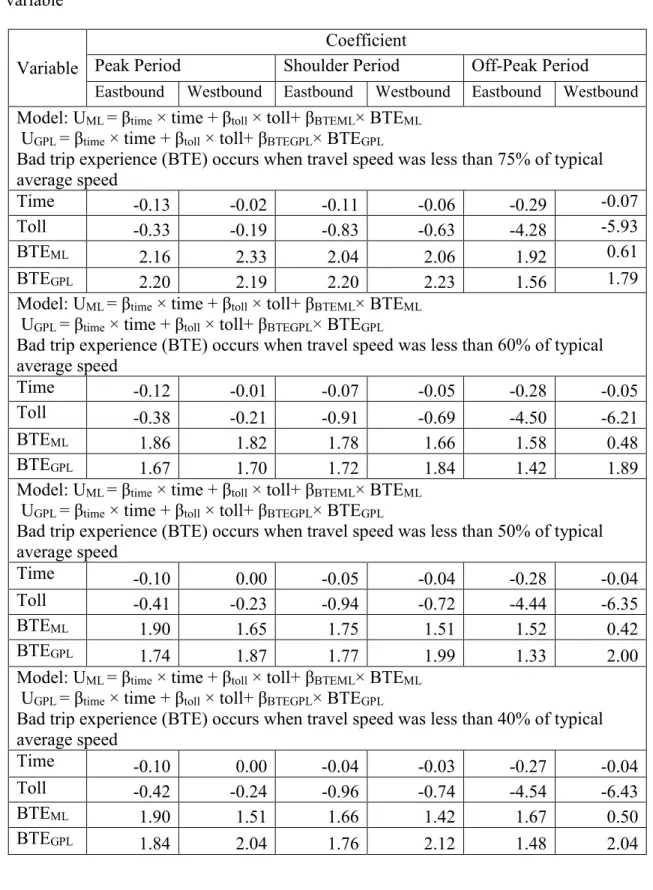
As the dataset allowed tracking all trips for a traveler on the Katy freeway, it provides an opportunity to see if a bad trip experience has an effect on his/her reliability perception or lane choice. For example, a bad trip experience on GPLs can lead a
33
traveler to choose MLs for future trips. Perception of a bad trip experience may vary from traveler to traveler. To define a bad trip experience, the travel speed of that trip will be compared with the average speed during that time of day. The average speeds will be calculated for every 10 minute interval using the three years of travel data .In this study, a trip will be considered as a bad trip when the travel speed of that trip is less than a percentage (in this case 40%, 50%, 60%, and 75%) of the average travel speed.
Other trip attributes, such as number of trips on each lane which are indicators of travelers’ familiarity with traffic condition on the Katy freeway, can be incorporated in the choice model. Familiarity with the traffic condition during a particular time of a day in certain direction can influence travelers’ lane choice decision. For example, a traveler may choose managed lane in westbound direction during peak period because of his familiarity with bad traffic conditions during that time. Due to the size of the dataset it is possible to calculate traveler familiarity variable for each direction of traffic (eastbound and westbound) and time period (peak, off-peak and shoulder) separately. Models will be developed to see how the travelers’ familiarity with the freeway and recent bad trip experience can affect their lane choice decision.
34
5.
DATA ANALYSIS
5.1 Processing of Data
5.1.1 Cleaning, Merging and Randomization of Data
The data generated form AVI sensors were obtained from two sources: TxDOT and HCTRA. The first step was to remove all attribute other than transponder ID, time stamp and sensor ID from both dataset. Then all entries with a missing attribute were removed and two dataset were merged to obtain raw AVI dataset. The raw AVI dataset had three attributes: transponder ID, sensor ID, and date and time of detection.
To make sure that no transponder owner could be identified using the transponder IDs, each transponder ID was replaced by a unique random ID. Therefore, the dataset could never be used to identify a specific individuals traveling on the Katy Freeway, but the dataset could still be used to track the trips of vehicles throughout the three years based on the random ID that each vehicle was assigned.
5.1.2 Exclusion of Specific Entries
To estimate a logit model for lane choice, it was necessary to have details for trips in both lanes. This meant generating trips in alternate lane (MLs for GPLs and vice versa). Therefore, each AVI sensor passed as a part of a trip was matched with a sensor on the alternate lane group to generate an alternate trip. Moreover, there are more AVI sensors on MLs than on the GPLs, which results in having more than one alternate ML sensor for some of the GPL sensors( for example, for GPL sensor number 443 there are
35
two alternate sensors on the MLs: 451 and 103). To address this discrepancy, the records obtained from the five TxDOT operated sensors (451, 454, 455, 458, and 459) were removed from data.
5.1.3 Trip Identification
Based on the AVI reads the trips of all vehicles with transponders along the freeway can be estimated. Individual AVI records can be matched together to form a collective series of points that represent a trip along the freeway. It should be noted that some GPL trips were not accurately recorded, as the AVI sensors operated by TxDOT were not originally designed to achieve 100% accuracy. The total numbers of missing data are unknown. However, millions of other trips were identified; therefore the sample is large enough to perform the analysis.
Travel time and distance traveled on the freeway were calculated using the time and location of the sequential detection of unique IDs. If the time difference between two consecutive detections was more than 15 minutes, those two detections were considered as part of two separate trips. It was assumed the vehicle exited the freeway, possibly to purchase gas, coffee, etc., and then returned to the freeway. Table 5shows the number and percentage of trips that would have decreased if a different time limit (20, 30, 40, 50, 60 minutes) were considered. Based on the fact very few additional trips would be added if the time limit were raised, it seemed that a 15 minute time limit would be reasonable
36
Table 5 Decrease in the number of trips based on time limit between detection
Time limit Decrease in the Number of Trips Percentage change in number of trips
20 1640 0.01%
30 19451 0.08%
40 64303 0.28%
50 111452 0.48%
60 140156 0.60%
* Three years of data (peak and shoulder period only) were considered and there were 23364508 trips during this period
* In the study 15 minutes were considered
5.1.4 Assigning Tolls and Removing HOV Trips
A toll was assigned to a trip when it was detected at one of the toll plazas. The toll was based on the time of detection and the corresponding toll value in the toll schedule (Table 4). As mentioned in an earlier section, during HOV-free hours HOVs can use the managed lane for free. Therefore, a vehicle detected by the HOV sensor during HOV-free hours was deleted from the dataset.
5.1.5 Alternate Trip Generation
For each trip an alternate trip was generated. This means if a traveler made a trip on MLs, his/her alternate trip would be a trip made during same time on the GPLs, and vice versa. The alternate trip should pass through the same freeway section but on the other set of lanes (GPL for ML trips and ML for GPL trips). It was assumed that the start time of an actual trip and its alternate trip were the same. The length of the alternate trip
37
varied a small amount (up to 0.3 miles) depending on the relative location of sensors on both sets of lanes. The two trips were made equivalent by multiplying the travel time and some reliability measures for the alternate trips by the ratio of the actual trip length to the alternate trip length. For example, assume the actual trip was on the GPLs and the sensors were spaced 1 mile apart. Then the alternate trip would be on the MLs. If the corresponding ML sensors were located 1.1 miles apart then some ML data would be multiplied by 0.91 (1/1.1) to adjust it to be equivalent to the trip on the GPLs.
Table 6 Average travel speeds by period
Period
Average Speed on the Toll Lanes
(in mph)
Average Speed on the GPLs
(in mph)
Peak Period 53.1 40.8
Shoulder 61.8 55.1
Off-Peak Period 70.9 65.3
* The speed comparisons are for the entire trip identified, which may include short parts of the trip that are outside the 12 miles of the toll lane
Depending on the data availability, alternate trips can be divided into three types. Travel times were calculated for each simulated trip by averaging travel times for similar freeway trips on the alternative lane (the lane that was not chosen). The simulated trips had to occur within the same 10-minute interval in which the actual trip was made. Average trip speeds were used when no trips could be found from the alternative lane
38
type. In this case, average speeds were calculated using actual trips during the same time frame (off-peak, shoulder and peak), averaged across an entire month (see Table 6).
The three types are:
1. Alternate trip type 1: Data from other travelers’ actual trips were available to calculate the attributes of alternate trips.
2. Alternate trip type 2: Data from other travelers’ actual trips were available in majority, but not all, segments in the alternate lane. For example, to calculate the attributes of an alternate trip (A-B-C-D) , when data from other travelers’ actual trips were available in the segment of A-B and C-D and no actual trip identified during that time in the segment of B-C, travel time of B-C segment was approximated using average travel speed (see Table 6) and length of segment.
3. Alternate trip type 3: No actual trips were found in any segment of the potential alternate trip. Travel time was approximated using average travel speed (see Table 6) and length of segment.
Only 1.3% of the alternate trips’ travel times were approximated during peak hours and 7.8% during the off-peak hours.
39 Table 7 Number of alternate trips by type
Time of Day Type 1 Type 2 Type 3
Peak Hour 6014328 5929876 155378
Shoulder Hour 4004626 7077018 183282
Off-Peak Hour 9194560 62877649 6093964
Table 8 Percentage of alternate trips by type
Time of Day Type 1 Type 2 Type 3
Peak Hour 49.7% 49.0% 1.3%
Shoulder Hour 35.5% 62.8% 1.6%
Off-Peak Hour 11.8% 80.4% 7.8%
5.1.6 Travel Time Reliability
In this study, reliability was based on the variability of travel times over the 20 weekdays prior to a given trip. To calculate the reliability measures for a given time of day and section of freeway, several statistical values such as mean, median, standard deviation and percentile (10th, 25th, 50th, 75th, 80th, 85th, 90th, and 95th) values of the travel time over the previous 20 weekdays were needed.
Reliability measures were calculated for every 10 minutes. The required statistical values of travel time between a given pair of sensors for a given time interval on a
40
specific day were calculated using the average travel times observed during the previous 20 weekdays. For example, to calculate reliability for a trip between sensors 465 and 444 (see Figure 2) during 12:00 pm-12:10 pm on July, 29th 2012, the first step was to
calculate average travel time observed between sensors 465 and 444 during 12:00 pm-12:10 pm on each weekday from July 1st to July 28th . The required statistical values were then calculated using these average travel times. Ideally there should be 20 travel times to use to calculate the reliability measures. However, there were often less than 20 days with traffic during specific periods of the day at specific locations - particularly overnight. If there were less than 3 days of data available then there was insufficient data to determine the reliability for that specific 10-minute period. This removed
approximately 4% of the overall trip data. It should be noted that, in some cases, no trip was observed starting and ending at a pair of sensors located close together, as vehicles were traveling longer distances. In those cases the average travel time between a pair of closely-located sensors was approximated using data from longer trips, given that the travelers who made those longer trips also passed the closely-spaced sensors. Suppose, on a specific day during 12:00 pm -12:10 pm, there were no trips that started at sensor 443 and ended at sensor 466 (see Figure 2). However, on that day during that time period, there might be many trips from sensor 465 to sensor 466, from sensor 443 to sensor 444, or from sensor 465 to sensor 440. Form the trip data between the pairs of sensors mentioned above, the time required to travel between sensor 443 and 466 could be estimated based on the speeds of vehicles traveling between 465 to 466, 443 to 444,
41
and 465 to 440. The estimated speed could be used to approximate the average travel time between sensor 443 and 466 during that that specific 10-munite period.
The free flow travel time was required to calculate some of the reliability measures. The free flow travel time is a function of free flow speed and trip length. The free flow speed is the speed of a traffic stream when the traffic density is very low. For this study, the median speed of vehicles that traveled between 11:00 pm and 12:00 pm during weekends in July 2012 and August 2012 was used as the free flow speed. The result suggests that the free flow speed was 68.8 mph on the managed lanes and 67.1 mph on the general purpose lanes.
5.2 Overview of Paid ML Trips
This section will discuss the initial examination of the general size and scope of the data used in this analysis. Approximately 3 million trips per month were assessed. The numbers of trips recorded during the three-year period are shown in
Table 9. It should be noted that these data exclude trips taken by vehicles without transponders, free ML trips (e.g. carpools or HOVs), and trips where the location of sensors restricted the capability of determining where a trip had occurred. Despite the high number, the sample is only a fraction of all Katy Freeway trips taken during the three-year period. However, this dataset should be well beyond what is needed to estimate travelers’ willingness to pay for travel time savings and reliability, considering previous research has been based on a few hundred to a few thousand travelers.
42 Table 9 Number of recorded trips
Year Number of Trips on the General Purpose Lane Number of paid Trips on the
Managed Lane Total Trips 2012 (January - November) 31,247,230 2,011,608 33,258,838 2013 (January - December) 36,017,349 2,601,242 38,618,591 2014 (January - September) 32,053,989 2,400,737 29,653,252
The number and percentage of paid ML trips are shown in Table 10. A surprisingly large number of trips, almost 3.4 million, use the MLs during the off-peak period. This represents only 4.31% of the total trips recorded during the off-peak period. During peak hours the use of MLs increased significantly, 19.28% of transponders detected during the peak periods used the MLs. Figure 3 presents the toll those trips paid, and Figure 4 shows the travel time savings.
Table 10 Paid trips on managed lane
Time Period (see Table 4 for
times of day) Number of Trips on the Managed Lanes
Percentage of All Trips that Were Paid Trips on the Managed Lanes
Off-Peak 3,379,635 4.31%
Shoulder 1,300,189 11.55%
43 0 2 4 6 8 10 12 14 16 18 20 0.3 0 0.7 0 1.0 0 1.3 0 1.4 0 1.7 0 1.8 0 2.1 0 2.4 0 2.6 0 2.8 0 3.2 0 3.4 0 3.6 0 3.9 0 4.4 0 4.9 0 5.2 0 5.9 0 6.6 0 P er ce n tage of T rip s Toll Paid ($)
Figure 3 Total toll paid on the managed lanes
Figure 4 Travel time saved (minutes) on the managed lanes 0 10 20 30 40 50 60 70 80 90 100 -3 -2 -1 0 1 2 3 4 5 6 7 8 9 10 11 12 13 14 15 16 17 18 19 20 Cu m u lativ e Pe rc e n tage o f Tr ip s
44
The travel time saved on MLs ranged from -3.3 minutes (the MLs were slower) to over 20 minutes. Approximately 11% of all paid trips on the MLs did not save any travel time. The average travel time savings was 2.6 minutes. It should be noted that there were many short trips on the MLs (as can be seen from the tolls paid in Figure 3) and this likely accounts for many of the smaller time savings. The travel time savings were not similar in both directions. Westbound traffic averaged twice as much travel time savings as east bound traffic on the MLs (see Table 11). If the time saved for a specific ML trip is divided by the toll paid on that trip the result is shown in Figure 5.
Table 11 Travel time saving on the managed lane
Travel time savings (minutes)
Travel time savings (minutes per mile)
Eastbound Westbound Eastbound Westbound
Peak 2.7 5.9 0.4 0.7
Shoulder 1.7 3.6 0.2 0.4
off-Peak 0.7 1.4 0.1 0.2
Figure 6 summarizes the number of trips by the length driven in the study corridor. It should be noted that the length of a trip presented here is based on the location of sensors, so it is not possible to know their actual origin and destination, or the entire length of the trip. The most common trip length was between 4 miles to 8 miles. As trip length increased above 8 miles, the number of those trips decreased.
45 Figure 5 Toll paid divided by time saved
.
Figure 6 Number of trips by length 0 10 20 30 40 50 60 70 80 90 100 -150 -50 50 150 250 350 Cu m u lativ e Pe rc e n tage
Toll Paid ($) / Time Saved (Hour)
0 5000000 10000000 15000000 20000000 25000000 30000000 35000000 40000000 0-4 4-8 8-12 12-16 16-20 20+ Num ber of t rips
Length of trips ( in miles)
ML GPL