Edinburgh Research Explorer
A Practical Guide for the Effective Evaluation of Twitter User
Geolocation
Citation for published version:
Mourad, A, Scholer, F, Magdy, W & Sanderson, M 2019, 'A Practical Guide for the Effective Evaluation of
Twitter User Geolocation', ACM Transactions on Social Computing (TSC), vol. 2, no. 3, 9.
https://doi.org/10.1145/3352572
Digital Object Identifier (DOI):
10.1145/3352572
Link:
Link to publication record in Edinburgh Research Explorer
Document Version:
Peer reviewed version
Published In:
ACM Transactions on Social Computing (TSC)
General rights
Copyright for the publications made accessible via the Edinburgh Research Explorer is retained by the author(s)
and / or other copyright owners and it is a condition of accessing these publications that users recognise and
abide by the legal requirements associated with these rights.
Take down policy
The University of Edinburgh has made every reasonable effort to ensure that Edinburgh Research Explorer
content complies with UK legislation. If you believe that the public display of this file breaches copyright please
contact [email protected] providing details, and we will remove access to the work immediately and
investigate your claim.
AHMED MOURAD,
School of Computer Science and Information Technology, RMIT University, AustraliaFALK SCHOLER,
School of Computer Science and Information Technology, RMIT University, AustraliaWALID MAGDY,
School of Informatics, The University of Edinburgh, United KingdomMARK SANDERSON,
School of Computer Science and Information Technology, RMIT University, AustraliaGeolocating Twitter users—the task of identifying their home locations—serves a wide range of community and business applications such as managing natural crises, journalism, and public health. Many approaches have been proposed for automatically geolocating users based on their tweets; at the same time, various evaluation metrics have been proposed to measure the effectiveness of these approaches, making it challenging to understand which of these metrics is the most suitable for this task. In this paper, we propose a guide for a standardized evaluation of Twitter user geolocation by analyzing fifteen models and two baselines in a controlled experimental setting. Models are evaluated using ten metrics over four geographic granularities. We use rank correlations to assess the effectiveness of these metrics.
Our results demonstrate that the choice of effectiveness metric can have a substantial impact on the conclusions drawn from a geolocation system experiment, potentially leading experimenters to contradictory results about relative effectiveness. We show that for general evaluations, a range of performance metrics should be reported, to ensure that a complete picture of system effectiveness is conveyed. Given the global geographic coverage of this task, we specifically recommend evaluation at micro versus macro levels to measure the impact of the bias in distribution over locations. Although a lot of complex geolocation algorithms have been applied in recent years, a majority class baseline is still competitive at coarse geographic granularity. We propose a suite of statistical analysis tests, based on the employed metric, to ensure that the results are not coincidental1.
CCS Concepts: •General and reference→Evaluation;
Additional Key Words and Phrases: Twitter, User Geolocation, Effective Evaluation, Statistical Analysis
ACM Reference Format:
Ahmed Mourad, Falk Scholer, Walid Magdy, and Mark Sanderson. 2019. A Practical Guide for the Effective Evaluation of Twitter User Geolocation.ACM Trans. Soc. Comput.1, 1, Article 1 ( January 2019),23pages.https://doi.org/10.1145/3352572
1 INTRODUCTION
Geolocating Twitter users is needed in many social media-based applications, such as identifying geographic lexical
variation [Eisenstein et al. 2010;Han et al. 2014], managing natural crises [Kryvasheyeu et al. 2015], gathering news [Liu
1
The code for the evaluation framework detailed in this article can be found on: https://bitbucket.org/amourad/geoloceval.git
Authors’ addresses: Ahmed Mourad, School of Computer Science and Information Technology, RMIT University, 124 La Trobe Street, Melbourne, VIC, 3000, Australia, [email protected]; Falk Scholer, School of Computer Science and Information Technology, RMIT University, 124 La Trobe Street, Melbourne, VIC, 3000, Australia, [email protected]; Walid Magdy, School of Informatics, The University of Edinburgh, 10 Crichton Street,Edinburgh, EH8 9AB, United Kingdom, [email protected]; Mark Sanderson, School of Computer Science and Information Technology, RMIT University, 124 La Trobe Street, Melbourne, VIC, 3000, Australia, [email protected].
Permission to make digital or hard copies of all or part of this work for personal or classroom use is granted without fee provided that copies are not made or distributed for profit or commercial advantage and that copies bear this notice and the full citation on the first page. Copyrights for components of this work owned by others than ACM must be honored. Abstracting with credit is permitted. To copy otherwise, or republish, to post on servers or to redistribute to lists, requires prior specific permission and /or a fee. Request permissions from [email protected].
© 2019 Association for Computing Machinery. Manuscript submitted to ACM
et al. 2016;Schwartz et al. 2015;Zubiaga et al. 2013], and tracking epidemics [Broniatowski et al. 2013;Dredze et al.
2013]. While users can record their location on their profile,Hecht et al.[2011] reported that more than 34% record fake
or sarcastic locations. Twitter allows users to GPS locate their content, however,Han et al.[2014] reported that less
than 1% of tweets are geotagged. Inferring user location is therefore an important field of investigation.
Each geolocation application has different needs, which might require evaluation from several perspectives. However,
current evaluation practices focus on a few measures introduced byEisenstein et al.[2010]. These measures were
shown to be biased towards densely populated (urban) locations [Mourad et al. 2017], e.g. the accuracy over urban
locations will dominate the overall measure. Such measures may be unsuitable to evaluate applications that treat urban
and rural locations with the same degree of importance: e.g. searching for sources to cover local news [Liu et al. 2016;
Schwartz et al. 2015;Starbird et al. 2012], monitoring natural disasters in rural areas [Kryvasheyeu et al. 2015], or
tracking epidemics in rural cities [Dredze et al. 2013].
Moreover, evaluation at multiple levels of geographic granularity is not widely used despite it being required by
some applications. For instance,Diakopoulos et al.[2012], in determining requirements from journalists for identifying
eyewitnesses from social media, found that aggregating predicted eyewitness location at different scales was requested,
e.g. city, state or country. Similarly,Dredze et al.[2013] presented a geolocation prediction system (Carmen) for influenza
surveillance, which predicts a structured location at different granularities.
The evaluation of geo-inference methods is affected by many factors, such as dataset availability, pre-processing,
ground-truth construction, geographic coverage, and how the earth is represented.
Analyzing the quality of fifteen geolocation models and two baselines, using ten different evaluation measures over
four geographic granularities, our study proposes a guide for the evaluation of Twitter user geolocation through the
following contributions:
• We standardize the evaluation process for models to ensure the fairness of comparison. We demonstrate that
some older models that were previously thought to be uncompetitive perform comparably to recent approaches.
• We examine the influence of social media population bias on the quality of geolocation prediction. In particular,
we find that a wide range of metrics and a majority class baseline should be used for the evaluation of more
complex geolocation models.
• We assess the effectiveness of current evaluation metrics using rank correlations. We demonstrate that the
ranking of user geolocation systems varies based on the evaluation metric and geographic granularity. In some
cases, some of the most common evaluation metrics are redundant and should not be used simultaneously.
• We validate the effectiveness of the proclaimed state-of-the-art geolocation systems using statistical significance
testing. We propose a suite of statistical significance tests suitable for the task at hand, based on the employed
metric.
• We study the degree to which metrics can lead to contradictory, yet statistically significant results, concluding
that systems should be evaluated using a range of measures.
This paper builds upon our own previously-published work [Mourad et al. 2018] with more statistical analysis
(effectiveness and significance) through the last three contributions. Our results demonstrate the different properties
of measures, which can in turn lead to a better understanding of the differences between models, and to better
decision-making based on specific application requirements.
2 RELATED WORK
Zheng et al.[2018] surveyed previous research on the geolocation of Twitter users. They reviewed and summarized all
geolocation methods and evaluation metrics employed from an empirical perspective. In this work, we present the
metrics from two different perspectives. We briefly introduce the different approaches of inferring a user’s location
in §2.1. In §2.2, we discuss how evaluation metrics for Twitter user geolocation evolved over time. This presentation
explains the original intuition behind each metric, reveals the decisions taken by subsequent researchers and the impact
of such choices on the evaluation process. We also chart the limitations and commonality of each metric. Examination
of biases in social media are detailed in §2.3. In §2.4, we survey efforts to standardize the evaluation process of Twitter
user geolocation and assess the effectiveness of the evaluation metrics employed.
2.1 Geolocation Methods
Previous research inferred the location of a Twitter user from different sources of information, namely tweet-text,
user’s social-network (e.g. followers, following, mentions) and meta-data (e.g. profile location, tweet timezone). Most
geolocation methods rely on the first two sources and hence are known in research as text-based and network-based
approaches. Text-based methods tend to address geolocation inference as a classification task. They rely on identifying
location indicative words (aka local words) over a predefined set of locations (e.g. administrative regions or grid cells).
Location sparsity is, therefore, a limitation of text-based approach. The intuition behind network-based methods is that
a user is geographically close to their friends. However, if a user is not covered in the training network, a geolocation
model will not be able to infer their location. Hence, recent research is focusing on a hybrid approach which combines
both approaches.
Jurgens et al.[2015b] constructed a benchmark for the network-based approach. They re-implemented the
state-of-the-art models, back at the time, and made it publicly available to the research community. In the process to do that,
they constructed their own dataset to train the models and ensure fairness of comparison. Recent research, however,
still prefer to reconstruct benchmark datasets which were created by the text-based research to evaluate their models,
than constructing their own datasets and retraining the available models. We, therefore, choose to focus on text-based
approaches to set a reliable benchmark process for the task of Twitter user geolocation regardless of the underlying
approach. We highlight the pitfalls of reconstructing Twitter datasets and comparing to results reported in previous
research.
2.2 Geolocation Metric Evolution
Table1details a chronological ordering of Geolocation Metrics, which we initially overview and then describe in more
detail.
2.2.1 Overview. Evaluation of geolocation models was initially measured usingMedianandMeanerror distances
between an estimated and true location [Eisenstein et al. 2010]. The researchers also used accuracy (Acc) at the level of
states (49) and regions (4). The choice of spatial granularity was influenced by the use of ground truth datasets, which
were drawn from the US (the country with the majority of Twitter users in 2010), and for a better interpretability of the
results compared to error distance.
Several metrics based on accuracy and/or error distance were introduced.Backstrom et al.[2010] evaluated
perfor-mance based on the fraction of predictions withinxkilometers from the true location using a Cumulative Distribution
Function (CDF) for all values ofxwithin 10,000 km. Accuracy withinxmiles from the original city was introduced by
Cheng et al.[2010], as was accuracy within the topkcities (Acc@k), and at the level of country by [Hecht et al. 2011].
Priedhorsky et al.[2014] introduced three new metrics, based on the error distance and the probability of estimation.
Rodrigues et al.[2016] reported precision and recall at the level of each city and an overall macro-F1 metric, which
was further extended byMourad et al.[2017] to consider micro, weighted, and macro averaging techniques at the
level of the three metrics. Other research employed a combination of these measures, as described in Table1. Given
thatAcc@k[Cheng et al. 2010] and the metrics introduced byPriedhorsky et al.[2014] were employed only in their
respective research, they were not presented in the table.
2.2.2 Accuracy Error.Cheng et al.[2010] showed empirically that 30% of users are placed within 10 miles of their true location, and 51% within 100 miles after exploring a range from 0 to 4,000 miles.
Subsequent research used the (perhaps) arbitrarily chosen range of 100 miles (161 km) to measure accuracy
(Acc@161) [Han et al. 2014;Roller et al. 2012;Wing and Baldridge 2014]. Note, the variance in accuracy with
re-spect to the range was tested on a dataset limited to the US. Using a population-based global earth representation,2the
average distance between cities and their neighbours was found to be in the range of 32–46 miles [Mourad et al. 2017],
less than half the 100 miles threshold. A system which predicts the location of a user two cities away from his/her home
location could be as accurate as a system which predicted the location one city away from the true location. This choice
of the tolerance distance questions the appropriateness ofAcc@161as a measure that suits global geographic models. A
somewhere arbitrary threshold is also found in the metricAuc, introduced byJurgens et al.[2015b], which quantifies
the graph generated by a CDF into a single number. This number is generated using the range value of 10,000km.
Error distance measures (Mean and Median) can be more accurate thanAcc@161because they are measured based
on the raw estimations of geolocation models without any approximation (discretization, e.g. map to a region such as a
city or country). However, they can exhibit a large variability on the measured results and limit evaluation at multiple
levels of geographic granularity, which is required by some geolocation applications as mentioned in §1. On the other
hand, metrics based on accuracy and error distance (e.g.Acc@161,CDF, andAUC) strongly depend on the distance
thresholds that are selected.
2.2.3 Dataset Availability.Table1(columns #Users and #Tweets) shows a large disparity in the sizes of test datasets. Although Twitter provides access to the public data generated by users, the terms of service limits the sharing of this
data to only tweet IDs. Any attempt to reconstruct a dataset used in previous research will be subject to decay, i.e. some
tweets will disappear because they have been deleted. In an effort to solve this issue, two approaches were proposed.
First,Jurgens et al.[2015a] proposed an evaluation framework where the dataset is hosted by a single operator.
An experimenter submits a request to the host along with a code. However, the cost to the host of maintaining this
service, the difficulty of the development process for the experimenter, and the unprotected intellectual property—the
ownership of the code—meant this proposal was not taken up.
Second,Han et al.[2016] provided a dataset of tweet IDs for a user geotagging shared task (named World). However,
one of the participant teams pointed out that the re-constructed dataset was missing∼25% of the data [Jayasinghe et al.
2016]. Systems are therefore highly likely to be trained on different datasets, based on the time they were re-constructed.
Subsequent research [Miura et al. 2017] highlighted the same issue using two different datasets (UTGeo and World).
2.2.4 Earth-representation.The importance of measures was illustrated when two different models were each found
to perform better using different reverse-geocoding technique.Han et al.[2014] demonstrated that a multinomial
2
https://github.com/tq010or/acl2013 Manuscript submitted to ACM
T able 1. An o ver vie w of past w ork. Pr ecision, re call and f1-scor e ar e combine d in the column PRF . For datasets, names in b old repr esent the original dataset, empty #Users and #T w eets cells means the size of the re constructe d dataset was not rep orte d in the resp ectiv e w ork, and Scop e refers to the ge ographical co verage . For testset, p er cent is the p er centage of users in the testset to the whole colle ction; #T pu is the minimum numb er of tw eets p er test user . Evaluation Metrics Datasets T estset A cc A cc@161 Me dian Mean PRF Name #Users #T w e ets Scop e #Users #T pu Eisenstein et al. [ 2010 ] ✓ ✓ ✓ Ge o T e xt 9.5k 380k US 1.9k (20%) Backstr om et al. [ 2010 ] CDF Ba ckstrom US Cheng et al. [ 2010 ] ✓ 0–4k ✓ Cheng 135k 4M US 5k (3.7%) 1000+ Wing and Baldridge [ 2011 ] ✓ ✓ Ge o T e xt US Roller et al. [ 2012 ] ✓ ✓ Ge o T e xt US ✓ ✓ ✓ U T Ge o 449k 38M Nth Am 10k (2.22%) Ahme d et al. [ 2013 ] ✓ Ge o T e xt US Han et al. [ 2014 ] ✓ ✓ ✓ U T Ge o Nth Am W orld 1.4M 12M Global 10k (0.71%) 10+ Wing and Baldridge [ 2014 ] ✓ ✓ ✓ U T Ge o Nth Am W orld Global 10+ Prie dhorsky et al. [ 2014 ] ✓ ✓ Ge o T e xt 9.5k 380k US 1.9k (20%) Jurgens et al. [ 2015b ] A uc ✓ Jurgens Ro drigues et al. [ 2016 ] ✓ ✓ Ro drigues 11.8k Brazil Han et al. [ 2016 ] [W -N U T] ✓ ✓ ✓ W orld 1.4M 12M Global 10k (0.71%) 10+ Rahimi et al. [ 2017 , 2016 , 2018 ] ✓ ✓ ✓ U T Ge o Nth Am 10k W orld 1.4M 12M Global 10k (0.71%) 10+ Miura et al. [ 2017 ] ✓ ✓ ✓ ✓ U T Ge o 279k 23.8M Nth Am 10k W orld 782k 9.03M Global 10k 10+ Mourad et al. [ 2017 ] ✓ ✓ ✓ ✓ ✓ W ORLD 947k Global T w Ar chiv e 1.5M Global Do et al. [ 2017 ] ✓ ✓ ✓ Ge o T e xt 9.5k >370k US 1.9k (20%) U T Ge o 450k 38M Nth Am 10k W ORLD 1.4M 12M Global 10k Ebrahimi et al. [ 2018 ] ✓ ✓ ✓ Ge o T e xt 9.5k 380k US 1.9k (20%) U T Ge o 450k 38M Nth Am 10k W ORLD 1.4M 12M Global 10k
naïve bayes model with feature selection performs better than logistic regression [Roller et al. 2012] using city-based
representation,Wing and Baldridge[2014] demonstrated the opposite using uniform grids.
2.3 Underlying bias
Social media is known to have substantial population biases [Mislove et al. 2011]. They relied on the US census data to
reveal the sampling bias in Twitter data based on the demographics of Twitter users, namely geographic distribution,
gender and race/ethnicity. Not many researchers explored the impact of this bias on either determining the most
effective models or evaluation metrics. Focusing on the geographic bias over the urban-rural spectrum, [Hecht and
Stephens 2014] explored three of the most common sources for geotagged information, — Twitter, Flickr and Foursquare.
They showed that there is a population bias towards urban regions.
The first attempt to assess the influence of population bias on the existing models — Twitter user geolocation — was
done by [Pavalanathan and Eisenstein 2015]. They explored the influence of Twitter user demographics — gender and
age — on the tasks of detecting lexical variation over geographic regions and text-based Twitter user geolocation, yet
relying on accuracy per category (e.g. male vs female) for evaluation.Johnson et al.[2017] further explored the impact
of geographic bias on the latter task. They differentiated between population bias, and structural bias introduced by
algorithmic design. To assess the impact of each of these biases, they explored different sampling techniques on a US
rural-urban county based dataset. They demonstrated that existing geolocation approaches perform significantly worse
for rural areas than for urban.
Relying on an external gazetteer (US census data, which might not be available for other countries), consolidating
geographic regions into two classes only (rural-vs-urban) and finally evaluation of individual categories (e.g. accuracy
of male vs female) limits the scalability of the analysis. Most of the recent work relies on datasets with global geographic
coverage, with hundreds and thousands of classes, and ignores the existence of biases while designing or evaluating
their models. We, therefore, believe that focusing on an enhanced and scalable evaluation metrics (macro averaging in
specific) should come first; to reveal such biases and assess their impact on the design of geolocation algorithms.
2.4 Comparing Geolocation Evaluation Metrics
Studies have analyzed the effectiveness of evaluation metrics of Twitter user geolocation.Jurgens et al.[2015b] conducted
a comparative analysis of nine geolocation models using a standardized evaluation framework. Their evaluation was
limited to a network-based geolocation approach using error distance measures (Auc and Median) and a network
specific measure, which does not generalize to other approaches, such as the widely-used text-based ones. More recent
work byMourad et al.[2017] pointed out that accuracy measures are biased towards locations with a large population.
Although they employed a wide range of metrics, their work was limited to a single geolocation model while focusing
on the influence of language rather than the effectiveness of the evaluation measures.
In this paper, we focus on the effectiveness of geolocation evaluation regardless of the underlying geolocation
approach or the language of text, which entails generalization challenges discussed in the next section. We evaluate the
relative performance of fifteen geolocation models and two baselines using all the metrics in Table1.
3 STANDARDIZED EVALUATION
In considering how to build a standardized evaluation, first, alternate metrics are described that address data imbalance.
Second, we examine significance tests to assess the statistical differences between the geolocation models under study.
Finally, a unified output format and reverse-geocoding method are employed to assure the fairness of comparisons.
3.1 Evaluation Metrics
Much past research treated the problem of geolocating Twitter users as a categorization task. Given the global geographic
coverage of such a task (typically thousands of locations), there is an inherent imbalance in the distribution of users
over locations.AccandAcc@161are biased towards regions with a high population (the majority classes) [Johnson
et al. 2017]. Hence, we investigate conventional measures for multi-class categorization [Sebastiani 2002;Sokolova
and Lapalme 2009], which were included partially byRodrigues et al.[2016] and fully byMourad et al.[2017] in the
context of Twitter user geolocation. We consider Precision (P), Recall (R) and F1-score (F1) using Micro (µ) and Macro
(M) averaging.Precisionis more favored in situations such as when journalists are looking for eyewitnesses within a
specific city [Diakopoulos et al. 2012].Recallis favored in situations such as when these journalists want to increase
the search pool [Starbird et al. 2012]. Both scenarios focus on a single location, where comparison at the micro and
macro levels is essential.
Evaluation metrics are categorized into three groups. Continuous evaluation is based on the estimated GPS coordinates
(p) of a user (u), and represented by median and mean error distances from the original gps-point ( ˆp). Discrete evaluation
is based on the resolved locations of a user (landlˆare the predicted and true locations, respectively), and represented by
accuracy, precision, recall, and f1-score using micro and macro averaging. Mixed evaluation is based on a combination
of continuous and discrete metrics, and represented by accuracy within 100 miles of the true location.
The evaluation metrics considered in this study are defined as:
Continuous evaluation.
ErrorDistance(u)=дreat_circle{pˆ,p} Median=mediannusers−1
i=0 {ErrorDistance(ui)} Mean=n 1 users nusers−1 Õ i=0 {ErrorDistance(ui)} Discrete evaluation. Acc=n1 users nusers−1 Õ i=0 1(li =lˆi) PM = 1 nlocations nlocations−1 Õ i=0 P(l=li,lˆ=l i) RM = 1 nlocations nlocations−1 Õ i=0 R(l=li,lˆ=l i) FM = 1 nlocations nlocations−1 Õ i=0 Fβ(l=li,lˆ=l i)
For micro averaging, all precision, recall and f1-score are identical to accuracy [Pedregosa et al. 2011].
Mixed evaluation. Acc@161(p,pˆ)= 1 nusers nusers−1 Õ i=0 1(ErrorDistanceui ≤161km)
3.2 Significance Tests
Dror et al.[2018] highlighted the importance of applying statistical significance tests in the field of Natural Language
Processing (NLP) to ensure that the experimental results are not coincidental. Given the range of NLP tasks and
effectiveness metrics that can be applied, different statistical tests are needed. Based on the decision tree algorithm
provided byDror et al.[2018] for statistical significance test selection, we choose a combination of parametric (t-test)
and sampling-free non-parametric tests (sign test, and Wilcoxon). Given the large size of our dataset, parametric tests
are applicable because the test statistic follows the normal distribution, and sampling-free tests are computationally
less expensive than sampling-based non-parametric tests.
AlthoughDror et al.[2018] surveyed a large number of NLP papers on different tasks, they did not consider the
category frequencies of the datasets. We, therefore, follow the recommendation ofYang and Liu[1999] who considered
the appropriate choice of significance tests to measure the statistical differences between categorization models trained
on datasets with skewed category distributions. Two types are considered:microandmacro tests.
Themicro testsconsidered in this study are the micro sign test (s) and proportions z-test (p) [Yang and Liu 1999].
The former is a binomial test for comparing two systems, A and B, based on binary decisions for all user/location
pairs. The latter is used for measures which are proportions: accuracy, precision, and recall. The z-test computation for
precision and recall is based on performance scores using micro averaging.
Themacro testsinclude macro sign test (S), macro t-test (T), and macro t-test after rank transformation (T’, a.k.a
Wilcoxon) [Yang and Liu 1999]. Macro tests were originally based on F1 scores per category as a unit measure, but
we employed them for precision and recall as well. The S-test is a binomial sign test used to compare two systems,
A and B, based on the paired F1 values for individual locations. While the S-test reduces the influence of outliers, it
may be insensitive in performance comparison because it ignores the magnitude of differences between F1 values.
Insensitivity issues are resolved in T by considering the absolute differences between paired F1 values in a relevance
t-test. However, T becomes sensitive when F1 values are unstable, specifically for low frequency locations. Finally, the
Wilcoxon T’ provides a compromise between S-test and T by considering the rank differences between paired F1 values
for individual locations.
We use two-sided versions of the tests, as they avoid prior expectation about the direction of the effect and are more
conservative.
3.3 Unified Output and Reverse-Geocoding
When comparing models, it is necessary to train and test on the same dataset and to use models that output the same
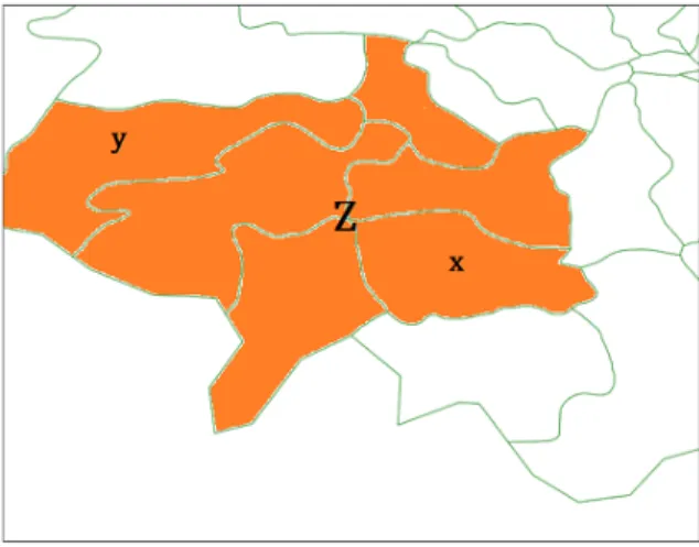
earth representation. Figure1shows an example of an unfair comparison between models producing different outputs
on the same dataset. Assume we have two models:AandB.Arepresents the earth as polygons (green outlined cells) and
Brepresents the earth as cities. A user’s home location is identified as polygonxinside cityZ(the orange area). Now
assumeApredicted the location of this user asy, andBpredicted it as cityZ. Based on the underlying representation of
each model, the prediction of modelAwill be considered incorrect while the prediction of modelBis correct.
In order to avoid such inconsistency, we unified the output of all the models to be GPS coordinates as suggested
by [Jurgens et al. 2015a]. We additionally resolved the coordinates to a location using a single online reverse-geocoding
API3before evaluation. Using a single reverse-geocoding API not only guarantees a fair comparison over the same set of
3
There is a trade-off between replicability, efficiency and cost, when choosing a reverse-geocoding API. An offline reverse-geocoding would be fast, but requires implementation and sharing the code base. On the other hand, online reverse-geocoding is easy to consume, but limited by a specific number of
Fig. 1. Example of unfair comparison between systems with different underlying earth representations. Cellxis the home location of a user and cellyis the predicted location by systemA. The orange cells represent the home and predicted city (Z) of a user by systemB.
locations (classes), it also allows evaluation over different granularities. In this work, we report the model performance
at city and country level. We calculated county and state level as well, but trends are consistent.
4 EXPERIMENTAL SETUP
We examine two sets of systems. The first set (Local) includes four geolocation models and two baselines, trained and
tested (over 30k users) locally over the same data collection with free earth representation to evaluate the considered
process. The second set (W-NUT) includes eleven submissions from a geolocation shared task, to assess the robustness
of our proposed metrics [Han et al. 2016]. Although the published results for participating models were evaluated at
city level only, we were able to infer output at country level based on information released by W-NUT organizers.
4.1 Local Models
4.1.1 Data Collection Method.We employed a geographically global geotagged tweet collection,TwArchive, holding
content since 20134drawn from the 1% sample Twitter public API stream. We used a 2014 subset spanning nine months.
We focus on English tweets only as identified by langid.py [Lui and Baldwin 2012]. Non-geotagged and duplicate
tweets were removed using user id and tweet text. For the sake of a standard evaluation, users with unresolved home
location—based on the model that accepts home locations in the form of cities instead of GPS coordinates [Han et al.
2014]—were removed from the dataset. The total number of users and tweets after pre-processing is∼1.5 million and
∼3.1 million respectively.
4.1.2 Ground Truth.The home location of a user was identified as the geometric median of their geotagged tweets [
Ju-rgens 2013]. Such a point is the minimum error distance to all locations of a user. The median has been shown to be
more accurate in identifying the home location of a user at a finer granularity than other approaches [Poulston et al.
2017]. The distance between any two GPS points is measured using the great circle distance method.
requests per day. Free APIs have a small limit, e.g. 2.5k requests per day for Nominatim, While commercial APIs have a larger limit, e.g. 100k requests per day for Google Reverse-Geocoding API V3. It took two weeks to reverse-geocode our local dataset of the size 1.5M users, using Google API.
4
https://archive.org/details/twitterstream&tab=collection
4.1.3 Geolocation Inference Models. Four models and two baselines were compared using four classification methods and two statistical methods. The models were chosen based on their availability, reproducibility, and recency.
Roller et al.[2012](Rl12) proposed an adaptive grid-based representation with a trained probabilistic language model
per cell. Each cell has the same number of users, but a different geographical area. We employ their best reported
parameter values for constructing the grid to retrain their model5on our local dataset. The output represents the
centroid of the predicted cell.
Han et al.[2014](Hn14) locates users to one of 3,709 cities. We re-implemented their system, focusing on the part
that uses Location Indicative Words (LIW) drawn from tweets, where mainstream noisy words were filtered out using
their best reported feature selection method, Information Gain Ratio. The output represents the centre of the predicted
city.
Rahimi et al.[2016](Rm16) assigns a user to one of 930 non-overlapping geographic clusters based on the similarity
of content. Their geotagging tool, Pigeo6, allowed retraining their text-based model on our local dataset. The output
represents the median of the predicted cluster.
Linear SVM(Lsvm) is a classic approach for imbalanced learning unlike Naïve Bayes. It is a variation of Hn14 by
replacing the classifier. The linear kernel is known to perform well over large datasets within a reasonable time.
Majority Class(Mc) is a baseline that always predicts the most frequent class in the training set.Yang[1999] pointed
out that in the case of a low average training instances per category (which applies here) themajority class trivial
classifiertends to outperform all non-trivial classifiers. It was used as a baseline in previous work [Han et al. 2014;
Mourad et al. 2017].
Stratified Sampling(Ss) is a baseline which picks a single class randomly biased by the proportion of each class in the
training set. Ss is expected to be a strong baseline for a classification task with multiple majority (or close to majority)
classes, unlike Mc which originated in binary classification.
Both baselines were implemented using scikit dummy classifier [Pedregosa et al. 2011] and output a class, not a
GPS coordinate. Measures that require a GPS coordinate to measure distance, Acc@161 and mean/median error, were
consequently not used to evaluate the baselines.
4.2 W-NUT Models
W-NUT7is a shared task for predicting the location of posts and users from a pre-defined set of cities [Han et al.
2016]. We analyze the results of eleven systems in the user geolocation prediction task (submitted by five teams). The
top two submissions were based on ensemble learning (Csiro.1) and neural networks (FujiXerox.2), making use of
multiple sources of information, including tweets, user self-declared location, timezone values, and other features. One
submission used tweet text only (Ibm). Two teams (Aist and Drexel) did not submit a description of their submissions.
5 RESULTS
Table2details the results of our experiments on two sets of systems (Local and W-NUT) across all metrics mentioned
in Table1; PRF (precision, recall, f1-score) are calculated usingµandMaveraging; using the output levels city and
country. Error distance metrics (Median and Mean) are measured between the home and estimated GPS coordinates of
a user. The best scoring systems for each metric are highlighted in bold.
5 https://github.com/utcompling/textgrounder/wiki/RollerEtAl_EMNLP2012 6 https://github.com/afshinrahimi/pigeo 7 https://noisy-text.github.io/2016/geo-shared-task.html Manuscript submitted to ACM
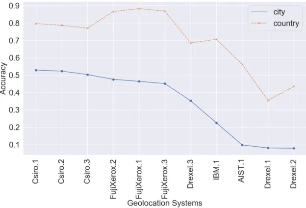
Fig. 2. Evaluation of W-NUT based-on accuracy at the levels of city and country, ordered by city in a descending order.
We first compare which systems are judged best under different evaluations, next we examine rank correlations of
systems, and finally study significant differences. For each experiment, we compare across output levels (i.e. city vs
country) and at the same output level (i.e. city or country).
5.1 Best system
We compare two forms of evaluation based on metric commonality as shown in Table1: most common metrics (Acc,
Acc@161, Median and Mean error distances) and alternate metrics (PRF usingµvsMaveraging).
5.1.1 Unified output influence using most-common metrics. The country and city representations are evaluated using two measures: Acc and Acc@161, which report different best performing geolocation models in the Local and W-NUT
sets at the city level, respectively. In terms of accuracy measures, results in the Local section of Table2show that Rl12
and Hn14 are competitive in terms of Acc at the level of city, while Rl12 achieves better results in terms of Acc at the
level of country and Acc@161 at both levels. On the other hand, the Lsvm model achieves the best Acc at the level of
city only .
To further illustrate the differences found when using city and country representations, the W-NUT systems,
measured using Acc, are shown in Figure2. Standardization enables the comparison of the best performance of each
geolocation model.
T able 2. Evaluation base d on all metrics at the le vel of city and countr y and sorte d in a descending or der of A cc. City Countr y Me dian Mean A cc A cc@161 Pµ Rµ F 1µ PM RM F 1M A cc A cc@161 Pµ Rµ F 1µ PM RM F 1M Local Lsvm 0.145 0.193 0.085 0.068 0.075 0.045 0.040 0.039 0.446 0.448 0.447 0.446 0.447 0.098 0.113 0.099 3656 5936 Rl12 0.128 0.228 0.114 0.050 0.070 0.036 0.020 0.023 0.615 0.619 0.621 0.615 0.618 0.144 0.138 0.133 1740 3785 Hn14 0.127 0.182 0.068 0.070 0.069 0.091 0.014 0.020 0.599 0.600 0.600 0.600 0.600 0.241 0.050 0.068 3128 4489 Rm16 0.074 0.132 0.030 0.021 0.025 0.007 0.001 0.001 0.315 0.316 0.315 0.315 0.315 0.062 0.015 0.015 5909 5653 Mc 0.018 0.000 0.018 0.020 0.019 0.000 0.000 0.000 0.523 0.000 0.523 0.524 0.523 0.004 0.007 0.005 — — Ss 0.002 0.000 0.003 0.002 0.002 0.001 0.000 0.000 0.301 0.000 0.302 0.302 0.302 0.007 0.007 0.007 — — W -N UT Csiro.1 0.529 0.636 0.544 0.529 0.537 0.545 0.432 0.454 0.798 0.799 0.798 0.798 0.798 0.661 0.538 0.568 21 1928 Csiro.2 0.523 0.619 0.544 0.523 0.533 0.555 0.434 0.458 0.787 0.789 0.788 0.787 0.787 0.653 0.535 0.561 23 2071 Csiro.3 0.503 0.585 0.529 0.503 0.516 0.576 0.422 0.455 0.771 0.773 0.772 0.771 0.771 0.662 0.530 0.560 30 2242 FujiXero x.2 0.476 0.635 0.481 0.476 0.478 0.358 0.279 0.289 0.866 0.868 0.866 0.866 0.866 0.692 0.519 0.562 16 1122 FujiXero x.1 0.464 0.645 0.468 0.464 0.466 0.313 0.253 0.253 0.883 0.886 0.884 0.883 0.884 0.634 0.514 0.542 20 963 FujiXero x.3 0.452 0.629 0.455 0.452 0.453 0.283 0.243 0.237 0.869 0.872 0.869 0.869 0.869 0.621 0.502 0.527 28 1084 Drexel.3 0.352 0.474 0.367 0.352 0.359 0.348 0.230 0.253 0.686 0.689 0.701 0.686 0.693 0.631 0.494 0.530 262 3124 Ibm.1 0.225 0.349 0.225 0.225 0.225 0.099 0.049 0.053 0.706 0.707 0.706 0.706 0.706 0.306 0.148 0.169 630 2860 Aist.1 0.098 0.199 0.103 0.098 0.100 0.123 0.052 0.063 0.562 0.564 0.565 0.562 0.564 0.297 0.107 0.137 1711 4002 Drexel.1 0.080 0.140 0.082 0.080 0.081 0.062 0.025 0.031 0.354 0.355 0.355 0.354 0.355 0.157 0.072 0.086 5714 6053 Drexel.2 0.079 0.135 0.082 0.079 0.080 0.056 0.024 0.029 0.435 0.435 0.443 0.435 0.439 0.168 0.072 0.090 4000 6161
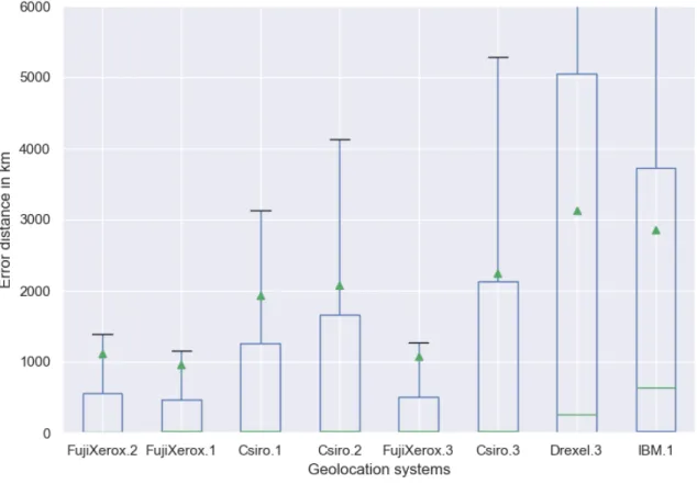
Fig. 3. Evaluation of W-NUT based-on error distance metrics (Median and Mean) in km.
We examine the error distance measures to try to understand the observed differences in best Local system. There is
a gap in performance between the grid based model (Rl12) and the city (Hn14 and Lsvm) or region/cluster (Rm16) based
models, see Table2. This gap is related to the geographic footprint per unit of the underlying earth representation.
Grid-based approaches tend to have the lowest error distances (because they are calculated from the center of the
predicted cell), followed by city-based, and finally region-based approaches.
For the W-NUT shared task, we observe that the FujiXerox submissions tend to have slightly better Acc@161 at the
level of city than the Csiro submissions (see Table2). At the level of country, however, the FujiXerox submissions
achieve much better results than Csiro, which is correlated to the gap in the mean error distance (in favor of FujiXerox
models) despite having competitive median error distance, as we will show later. Note that the original WNUT shared
task did not evaluate the participating systems at the level of country.
The distribution and results for the error distance measures are represented in more detail using a box plot in Figure3.
The green triangles represent the mean error distance for each system. An upper threshold distance of 6,000 km was
applied and the worst three systems (Aist.1, Drexel.1, and Drexel.2) were excluded so that details can be seen. We
can observe the large variance in 50-75% percentile between FujiXerox submissions and Csiro. Previous research [Han
et al. 2014;Melo and Martins 2017] promoted the usage of median error distance to evaluate user geolocation because it
is more robust to outliers than the mean, and easy to interpret the results in comparison to accuracy. However, the
boxplot quantifies the variance in error distance, and 25% can not be considered as outliers in this case. The mean error
distance therefore is a more effective measure than the median in this context. FujiXerox and Csiro submissions have
competitive results in terms of the median error distance, while FujiXerox submissions are much better in terms of the
mean error distance and have less variance in their estimations.
Results in the Local section of Table2show that the two baselines for the locally deployed geolocation models (Mc
and Ss) perform poorly at the level of city. In contrast, Mc establishes a strong baseline at the level of country, where it
performs much better than Rm16, Lsvm and Ss. Mc is effective at the level of country because of the lower number of
countries (few hundreds) compared to cities (few thousands). Given the large size of the training set (1.5 million), the
sparsity at the country level will be less, still with bias in the distribution, which also explains why the Naïve Bayes
based model (Hn14) performs better than Lsvm in this case. The Ss baseline performs poorly, which suggests it should
not be considered as a baseline. At this stage, the use of a simple Mc baseline and Acc did not reveal the influence
of imbalance as [Yang 1999] suggested. Therefore, we consider evaluation using different averaging techniques and
alternative measures to provide a better insight into the influence of imbalance.
5.1.2 Imbalance Influence using alternate metrics.The three evaluation measures (PRF) that use the two averaging
methods can be compared across city and country giving sixµvsMcomparisons. Across those six, the best system is
different in 67% and 100% of the comparisons in the Local and W-NUT sets, respectively.
A consistent drop in performance can be seen fromµtoM, see columnsPµ toF1Mof Table2. While Rl12 and Hn14
are competitive at the level of Acc, Rl12 tend to have higher precision than Hn14 using micro averaging, and vice versa
using macro averaging. Lsvm is another example where Acc is a limited measure when comparing to other systems.
While Lsvm achieves the best Acc at the level of city, it tends to have less precision than Rl12 using micro averaging
and Hn14 using macro averaging, yet has higher recall achieving the best F1-score among all systems in Local. Mc is
still competitive at the country level using micro averaging, achieving higher PRF than Rm16 and Lsvm.
If we consider both unified output and imbalance influences, in W-NUT, collectively the Csiro submissions outperform
FujiXerox at the level of city across all the evaluation metrics, except for Acc@161 and error distance measures. On
the other hand, FujiXerox submissions outperform Csiro at the level of country in terms of accuracy, micro averaging
and error distance measures, and vice versa using macro averaging, except for macro precision (PM).
To summarize the best system analysis, we demonstrated (in §5.1.1) that unifying the output format and
reverse-geocoding locations before evaluation are essential to ensure the fairness of comparison. A majority class baseline is
recommended at the country level in the case of using Acc or micro averaging method. The alternate metrics (macro
averaging in specific) should be used to evaluate the influence of data imbalance on the quality of geolocation prediction.
The question now is: how to quantify the effectiveness of using different evaluation measures?
5.2 Rank correlations
Kendall’sτis a correlation measure that quantifies the agreement between two ranked lists. We calculatedτBfor all
combinations of the employed metrics, see Figure4. Note, because the optimal value for distance metrics is 0 and the
optimal value for the other metrics is 1, the optimal correlation between those two is -1; the optimal correlation between
the non-distance metrics is 1. As the Local collection only includes four non-baseline systems, the range ofτBvalues is
limited, we therefore focus our analysis on the W-NUT data.
A strong correlation of any metric across different geographic granularities indicates the consistency of such a
measure in ranking geolocation models. On the contrary, a strong correlation between any two metrics at the same level
(a) Rank correlations across City and Country. Median and Mean error distances are excluded because geographic granularity is not applicable.
(b) Rank correlations at the level of City.
(c) Rank correlations at the level of Country.
Fig. 4. Kendall’sτBrank correlations between pairs of effectiveness metrics for the W-NUT collection,p<=0.05. Manuscript submitted to ACM
of geographic granularity (e.g. city) indicates less benefit from using both metrics at the same time. Hence, a moderate
or weak correlation suggests using both measures is important so a more complete picture of system effectiveness is
conveyed.
Considering city vs country (Figure4a), we observe a weak correlation between ranking models across city and
country using the commonly used Acc and micro averaging measures. Using macro averaging measures, a strong
correlation exists, similarly for Acc@161. This finding suggests that macro measures and Acc@161 are more robust for
comparison across geographic granularities.
Considering micro vs macro at the city level (Figure4b), we observe strong correlations across the three micro and
macro measures (0.8, 0.9, 0.9). Acc@161, median and mean error distances also have mutual strong correlations. On
the other hand, Acc, median and mean error distances have weak correlations. This contrast in correlations, therefore,
suggests not relying solely on measures driven from the error distance (Median, Mean, Acc@161) because they depend
on the underlying earth representation, i.e. grid-based representation will always achieve better results than city and
cluster based representations in terms of these metrics, even if the accuracy of city and cluster based models are better.
Considering micro vs macro at the level of country (Figure4c), we observe moderate correlations across the three
micro and macro metrics (0.6, 0.5, 0.6). The most common metrics (Acc, Acc@161, Median and Mean) and micro
averaging metrics tend to have strong correlations. On the other hand, they tend to have moderate correlations with
macro averaging metrics, except for the Median error distance. Therefore, a combination of micro and macro metrics or
most common metrics and macro metrics is recommended.
5.3 Statistical Significance
As was apparent from the system effectiveness scores in Table2, some of the results occurred within a close range.
Statistical significance tests are therefore important to establish confidence that differences are not just due to chance.
Following [Moffat et al. 2012], the outcome of a significance test will be categorized into one of two classes. Given
two models A and B, calculated for two metrics X and Y, suppose that significance tests are run on the models’ outputs
using both metrics. If they show statistically significant results for both metrics that system A is better than system B (or
vice versa), that would be considered a statistically significant active agreement (SSA). Statistical significant differences,
but with contradicting superiority on systems, would be considered a statistically significant active disagreement (SSD).
Figures5aand5bsummarize the results of the statistical significance tests for the W-NUT collection at the city
and country levels, respectively. Each figure summarizes the significant agreements and disagreements. The diagonal
values represent the percentage of systems pairs that are significantly different based on a single metric (discriminative
power), the values above the diagonal show the percentage of SSA, the values below the diagonal show the percentage
of SSD. As can be seen, there are many more agreements than disagreements.
Considering city vs country, we observe that the discriminative power of the evaluation metrics (on the diagonal)
and the percentage of SSA at the city level (above the diagonal) are always over 80% (see Figure5a). They are much
lower at the level of country for all comparisons involving macro tests (31–78%, see Figure5b), which suggests that
there is no huge difference in performance between geolocation models. On the contrary, the percentage of SSD (below
the diagonal) at the level of country is much lower than at the city level. These results support the importance of using
macro metrics for cross granularity evaluation suggested in the previous section.
Considering precision and recall, at the city level, the discriminative power (on the diagonal) using macro averaging
is better than micro; macro averaging is able to capture more statistically significant differences for both precision and
recall. At the country level, the opposite is true: micro measures are more discriminative than macro. The percentage of
(a) City-level
(b) Country-level
Fig. 5. Significant agreements and disagreements,p =0.05. W-NUT: 11 systems, 55 system pairs. Micro tests are s-Raw, p-Acc,
p-Pµ, and p-Rµ, while the rest represent Macro tests. Significance tests abbreviations stand for: s→sign-test, p→proportions z-test, S→macro sign-test, T→macro t-test, and T’→Wilcoxon test.
SSA involving micro metrics (first fours columns), above the diagonal, are observed to be higher than macro metrics.
The percentage of SSA involving macro metrics can drop down to 30.9%. The level of disagreements (SSD) are generally
low or zero. However, the occurrence rate is sometimes as high as 10.9% (for example, for T-PMand s-Raw at the city
level), similarly for tests involving macro metrics. These are cases where experiments would have led to contradictory
conclusions about statistically significant differences in system effectiveness, simply based on the metric that was
chosen for evaluation. For general evaluation, a macro-micro statistical significance comparison is recommended.
6 DISCUSSION AND LIMITATIONS
Datasets built using Twitter cannot be fully shared and are practically irreproducible because they are subject to decay
over time. This challenge will persist, unless Twitter changes their policy and the end-users give their consent to make
use of their data. Sharing datasets [Han et al. 2016], therefore, is not feasible. Building centralized frameworks where all
researchers submit their systems [Jurgens et al. 2015a], isn’t practical as well. Hence, every researcher will likely need
to create their own datasets, which will normalize the impact of confounding factors, such as data decay, pre-processing,
and ground-truth construction. However, this step requires other researchers to share their systems with the ability to
retrain their models.
The global geographic coverage of social media means that datasets are naturally imbalanced in terms of locations,
with bias towards big cities. Given that classification is a common approach to predict the location of a Twitter user,
it is important to highlight the large number of classes (thousands) involved in the learning process. For general
evaluation such as in Wnut shared-taskHan et al.[2016] or applications treating urban and rural locations with the
same degree of importance, a macro versus micro evaluation should be employed to address the limits of the most
common metrics (accuracy and error distance). A majority class baseline is also recommended at the level of coarse
geographic granularities, state and country in particular, as it achieved competitive results. Finally, we encourage
researchers to report the probability of their predictions/estimations, as opposed to binary classification outputs, to
allow for assessing the effectiveness of more evaluation metrics, such as CDF (§2.2) and Auc (§2.4).
With the large number of explored metrics, Kendall’sτ rank correlation test is recommended to quantify the
agreement between pairs of metrics. Our results showed that Acc@161, and macro metrics are more consistent and
highly correlated across different granularities in comparison to Acc and micro metrics. We demonstrated that error
distance metrics (Median, and Mean) and Acc@161 are dependent on the underlying earth representation. While they
are highly correlated at the same geographic granularity, they do not convey different information (redundant) and
error distance measures are insensitive to evaluation at several geographic granularities. Hence, they should not be
used as sole measures for evaluation, which is still the common practice [Bakerman et al. 2018;Ebrahimi et al. 2018;
Miura et al. 2017;Rahimi et al. 2018], specially using Acc@161 at fine granularities (city and county). A combination of
macro metrics (precision, recall and f1-score) and either micro metrics or accuracy and error metrics are recommended
for evaluation.
Statistical significance tests at micro and macro levels were employed to assess the effectiveness of the evaluation
metrics at both levels. Using SSA and SSD to summarize the outcome, our results revealed the disparity in agreements
and disagreements between tests based on the chosen evaluation metric and geographic granularity. The SSAs between
micro and macro tests are higher (better) at the level of city than country. The SSDs are higher (worse) at the level of
city than country. To the best of our knowledge, only few recent works applied statistical analysis [Miura et al. 2017],
and choosing the right tests can be challenging. Statistical significance testing is essential to draw robust conclusions
about the state-of-the-art. In the context of multi-classification and data imbalance, we recommend this list of two-sided
tests: i. Micro sign test (s) and proportions z-test (p) for micro evaluation using raw predictions, accuracy, precision
and recall. ii. Macro sign test (S), macro t-test (T), and Wilcoxon test for macro evaluation using precision, recall and
f1-score.
The choice of evaluation metrics should be justified by the needs of the applications and the underlying earth
representation. A standardized evaluation process, which unified the output format, allowed the comparison of systems
with different earth representations. We demonstrated that different systems were found to be best for different
underlying representations using an evaluation process including eight measures. Unlike previous research [Jurgens
et al. 2015b], evaluation after resolving the location of the unified output using a single reverse-geocoding API allowed
evaluation over four geographic granularities and ensured a fair comparison using the same set of locations and
avoided the mismatch of predictions based on different representations although they refer to the same location.
We demonstrated how competitive geolocation models—previously proclaimed to be inferior—could compete with
state-of-the-art models in terms of accuracy.
A major limitation to this work is not extending our evaluation process to network-based approaches, and more
importantly recent hybrid methods that rely on deep learning. User coverage is an essential network specific metric to
evaluate the percentage of test users with a predicted location [Jurgens et al. 2015b]. If a user does not have social ties,
a network-based geolocation model will not be able to predict a location. While hybrid approaches consider network
information for training, they evaluated their performance against text-based approaches using error distance measures
for two reasons. First, they rely on datasets constructed by text-based research. Second, they always predict a location
for a user; rely on text as a fallback if a user is disconnected. The challenge here is to address the user coverage aspect
when evaluating text-based against network-based approaches. In this case, recall could be a potential metric.
7 GEOLOCEVAL
Geocoding is the process of linking a document (e.g. Wikipedia article, web page, social media entity, etc.) to a location
on earth. Geocoding serves a wide range of applications. With ever increasing quantities of social media content, many
applications exploit such data. Examples include: dialectology (the study of geographic lexical variation of a language);
regional sentiment analysis; monitoring public health; managing natural crises; and the search for eyewitnesses
by journalists. Document geocoding has been an active research area over the last decade, resulting in hundreds of
publications, geocoding systems and datasets [Melo and Martins 2017;Mourad et al. 2018;Zheng et al. 2018]. Comparison
of such systems share the same challenges of Twitter user geolocation. We, therefore, share our evaluation framework
with the research community, hoping researchers will employ in their future geocoding research.
GeoLocEval is an open source python package8to evaluate the performance of a given set of geocoding systems.
The input is a list of JSON files, one for each system to be compared. Each file contains geolocations expressed in the
most generic format: GPS coordinates, as in Listing1. This format is compatible with the Twitter geolocation prediction
shared task at the level of tweets and users [Han et al. 2016], known as Wnut.
{ "doc_id": {"lon": "x", "lat": "y"}, }
Listing 1. JSON Input Format
The GPS coordinates are expanded using a single geocoding API. Results are exported to a JSON file, as in Listing2.
8
https://bitbucket.org/amourad/geoloceval.git
{ "483049821": { "geocoding_system_1": { "doc_id":"483049821", "lon":-74.0344411626724, "lat":40.74801738664574, "country":"United States", "county":"Hudson County", "state":"New Jersey", "city":"Hoboken", "error_dist":15137.622354338771 }, } }
Listing 2. JSON Output Format
7.1 Geocoding APIs
GeoLocEval supports two of the most common geocoding APIs used in previous research:
• Nominatim: a free OpenStreetMap based geocoder.
• GoogleV3: is a commercial API with a higher number of requests per day compared to Nominatim.
Each API supports four administrative levels, namely city, county, state and country. GeoLocEval caches all the resolved
GPS coordinates to reduce the number of requests.
7.2 Evaluation Process
We follow the process presented in §3, by first comparing systems under different evaluations and geographic granularity,
next examining rank correlations of systems, and finally studying significant differences. All the generated results are
exported to a text file.
8 CONCLUSION AND F UTURE WORK
The work in this paper examined the effectiveness of metrics employed in the evaluation of Twitter user geolocation
from three key aspects: standardized evaluation process, compensating bias due to population imbalance through micro
vs macro averaging, and comprehensive statistical analysis. We proposed a practical guide to follow for an effective
evaluation of each aspect based on thorough experiments and analysis encompassing fifteen geolocation models and
two baselines in a controlled environment.
A recommended practical guide for any new research on Twitter user geolocation includes: i) creating its own
dataset, ii) sharing its geolocation model with the ability to be retrained by the research community, iii) using a unified
output format (GPS coordinates), iv) using a single reverse-geocoding API for discrete evaluation of all the geolocation
models considered, v) employing a combined set of evaluation metrics at the micro and macro levels, vi) quantifying the
agreement between the evaluation metrics through rank correlation and vii) verifying the conclusions by conducting
the recommended statistical significance tests.
This work was initially motivated byGao and Sebastiani[2015] who changed the perspective of evaluating sentiment
analysis after many years of research. They argued that any study dealing with sentiment analysis is usually interested
in the sentiment at the aggregate level of classes, not at the individual level. Quantification-specific evaluation metrics
therefore should be used instead of classification metrics, based on the goal of the applications. Since Twitter user
geolocation applications do not have a unified goal as sentiment analysis, we focused on experimental evaluation using
a wide range of metrics as a vital step that leads to application-specific evaluation. For future work, we would like to
investigate the evaluation of geolocation models analytically. Instead of anticipating the needs of the applications, we
are interested in collaboration with domain experts, such as journalists, or humanitarians to develop the needs and
evaluation metrics in the context of a specific task.
Evaluation of geolocation models on datasets with different characteristics or domains to ensure their consistent
performance is a common practice.Rahimi et al.[2018] evaluated their models on three Twitter datasets with different
geographic coverage and size.Mourad et al.[2017] evaluated their model on Twitter datasets for thirteen different
languages.Wing and Baldridge[2014] evaluated their models on six datasets from different domains, namely Twitter,
Wikipedia and Flickr. In this paper, we measured the statistical significance of the differences between geolocation
models evaluated on the same dataset. For future work, we would like to extend our geolocation evaluation guide to
include the replicability analysis for statistical significance analysis over multiple datasets [Dror et al. 2017].
REFERENCES
Amr Ahmed, Liangjie Hong, and Alexander J Smola. 2013. Hierarchical geographical modeling of user locations from social media posts. InProceedings of the 22nd international conference on World Wide Web. 25–36.
Lars Backstrom, Eric Sun, and Cameron Marlow. 2010.Find me if you can: improving geographical prediction with social and spatial proximity. In Proceedings of the 19th international conference on World Wide Web. 61–70.
Jordan Bakerman, Karl Pazdernik, Alyson Wilson, Geoffrey Fairchild, and Rian Bahran. 2018. Twitter geolocation: A hybrid approach.ACM Transactions on Knowledge Discovery from Data (TKDD)12 (2018), 34.
David A Broniatowski, Michael J Paul, and Mark Dredze. 2013. National and local influenza surveillance through Twitter: an analysis of the 2012-2013 influenza epidemic.PloS one8 (2013), e83672.
Zhiyuan Cheng, James Caverlee, and Kyumin Lee. 2010. You are where you tweet: a content-based approach to geo-locating twitter users. InProceedings of the 19th ACM international Conference on Information and knowledge Management. 759–768.
Nicholas Diakopoulos, Munmun De Choudhury, and Mor Naaman. 2012.Finding and assessing social media information sources in the context of journalism. InProceedings of the SIGCHI conference on Human Factors in Computing Systems. 2451–2460.
Tien Huu Do, Duc Minh Nguyen, Evaggelia Tsiligianni, Bruno Cornelis, and Nikos Deligiannis. 2017. Multiview Deep Learning for Predicting Twitter Users’ Location.arXiv preprint arXiv:1712.08091(2017).
Mark Dredze, Michael J Paul, Shane Bergsma, and Hieu Tran. 2013. Carmen: A twitter geolocation system with applications to public health. InProceedings of the AAAI workshop on expanding the boundaries of Health Informatics using AI, Vol. 23. 20–24.
Rotem Dror, Gili Baumer, Marina Bogomolov, and Roi Reichart. 2017. Replicability Analysis for Natural Language Processing: Testing Significance with Multiple Datasets.Transactions of the Association of Computational Linguistics5 (2017), 471–486.
Rotem Dror, Gili Baumer, Segev Shlomov, and Roi Reichart. 2018. The hitchhiker’s guide to testing statistical significance in natural language processing. InProceedings of the 56th annual meeting of the Association for Computational Linguistics. 1383–1392.
Mohammad Ebrahimi, Elaheh ShafieiBavani, Raymond Wong, and Fang Chen. 2018. Twitter user geolocation by filtering of highly mentioned users. Journal of the Association for Information Science and Technology69 (2018), 879–889.
Jacob Eisenstein, Brendan O’Connor, Noah A Smith, and Eric P Xing. 2010. A latent variable model for geographic lexical variation. InProceedings of the 2010 Conference on Empirical Methods in Natural Language Processing. 1277–1287.
Wei Gao and Fabrizio Sebastiani. 2015. Tweet sentiment: From classification to quantification. InProceedings of the 2015 IEEE/ACM international conference on Advances in Social Networks Analysis and Mining 2015. 97–104.
Bo Han, Paul Cook, and Timothy Baldwin. 2014. Text-based twitter user geolocation prediction.Journal of Artificial Intelligence Research49 (2014), 451–500.
Bo Han, Afshin Rahimi, Leon Derczynski, and Timothy Baldwin. 2016. Twitter geolocation prediction shared task of the 2016 workshop on noisy user-generated text. InProceedings of the 2nd Workshop on Noisy User-generated Text. 213–217.
Brent Hecht, Lichan Hong, Bongwon Suh, and Ed H Chi. 2011. Tweets from Justin Bieber’s heart: the dynamics of the location field in user profiles. In Proceedings of the SIGCHI conference on Human Factors in Computing Systems. 237–246.
Brent J Hecht and Monica Stephens. 2014. A Tale of Cities: Urban Biases in Volunteered Geographic Information.. InProceedings of the eighth international AAAI Conference on Web and Social Media. 197–205.