Repositorio Institucional de la Universidad Autónoma de Madrid
https://repositorio.uam.es
Esta es la
versión de autor
del artículo publicado en:
This is an
author produced version
of a paper published in:
Pattern Recognition 45.12 (2012): 4414 – 4427
DOI:
http://dx.doi.org/10.1016/j.patcog.2012.06.002
Copyright:
© 2012 Elsevier B.V.
El acceso a la versión del editor puede requerir la suscripción del recurso
Access to the published version may require subscription
Hierarchical Linear Support Vector Machine
I. Rodriguez-Lujana,∗, C. Santa Cruza, R. HuertabaDepartamento de Ingenier´ıa Inform´atica and Instituto de Ingenier´ıa del Conocimiento, Universidad Aut´onoma de Madrid, 28049 Madrid, Spain.
bBioCircuits Institute, University of California San Diego, La Jolla CA 92093-0404, USA.
Abstract
The increasing size and dimensionality of real-world datasets make it necessary to design efficient algorithms not only in the training process but also in the prediction phase. In applications such as credit card fraud detection, the classifier needs to predict an event in 10 milliseconds at most. In these environments the speed of the prediction constraints heavily outweighs the training costs. We propose a new classification method, called a Hierarchical Linear Support Vector Machine (H-LSVM), based on the construction of an oblique decision tree in which the node split is obtained as a Linear Support Vector Machine. Although other methods have been proposed to break the data space down in subregions to speed up Support Vector Machines, the H-LSVM algorithm represents a very simple and efficient model in training but mainly in prediction for large-scale datasets. Only a few hyperplanes need to be evaluated in the prediction step, no kernel computation is required and the tree structure makes parallelization possible. In experiments with medium and large datasets, the H-LSVM reduces the prediction cost considerably while achieving classification results closer to the non-linear SVM than that of the linear case.
Keywords: Large-Scale Learning, Real-Time Prediction, Support Vector Machine, Decision Tree, Pegasos Algorithm
1. Introduction
1
Support Vector Machines (SVMs) have been widely used in classification problems as a result of their 2
effectiveness. However, the increasing size of real-world datasets in domains such as bioinformatics, document 3
categorization or credit card fraud detection compromises their application. The computational complexity 4
of the SVM decision function scales with respect to the number of support vectorsnSV and Steinwart [1]
5
showed that the number of support vectors scales linearly with respect to the number of training patterns. 6
Consequently, other machine learning techniques are preferred in those large-scale domains in which an 7
∗Corresponding author. Instituto de Ingenier´ıa delConocimiento; C/Francisco Tom´as y Valiente,11; E.P.S., EdificioB;
UAM-Cantoblanco, 28049Madrid,Spain. Tel: +34 91 497 2339; fax: +34 91 497 2334
Email addresses: [email protected](I. Rodriguez-Lujan),[email protected](C. Santa Cruz),
[email protected](R. Huerta)
*Manuscript
efficient prediction step is needed, especially in real-time applications such as credit card fraud detection 8
which requires a response time of less than 10 milliseconds. 9
Although the machine learning community has been mainly focused on speeding up the training of 10
the SVM, the emergence of applications requiring fast classification makes the design of new algorithms 11
necessary whilst maintaining as much as possible the effectiveness of non-linear SVMs and improving its 12
classification complexity at the same time. Linear SVMs are the best alternative for fast execution because 13
their decision boundary is made up of a single hyperplane. However, their performance for non-linear 14
problems is uncompetitive and a compromise between performance and classification speed is needed. 15
The computational complexity of testing a pattern using a non-linear SVM isO(nSV ×d×nK) where
16
nSV are the number of support vectors,dis the dimension of the samples andnK is the cost of evaluating
17
the kernel function. In large-scale problems, the number of support vectors is usually much higher than the 18
dimension of the problem (nSV ≫d) which is why almost all methods proposed in the literature aim at
19
reducingnSV. The methods for reducing the number of support vectors can be divided into two groups [2]:
20
• Numerical techniques find a reduced set of basis functions necessary to classify a pattern. These 21
algorithms usually consider all of the training patterns andfind a sparse representation of the support 22
vectors. A more detailed overview of these methods is given by Keerthi et al. [2]. According to 23
Keerthi’s categorization, the support vector reduction can be carried out as a post-processing phase 24
after training the SVM model or during the training phase thus imposing a certain sparsity in the 25
basis functions. The post-processing techniques ([3, 4]) reduce the number of support vectors once 26
the SVM model has been trained. Therefore, they still depend on the standard SVM training which 27
can be extremely costly in large-scale problems. Among the direct simplification approaches based 28
on imposing sparseness on the basis functions in the primal space, several methods can be found in 29
the literature [5, 6, 2]. These approaches considerably reduce the SVM prediction cost while having 30
a competitive classification accuracy, but in some datasets the number of basis functions needed to 31
maintain a competitive classification accuracy is still high for efficient training and prediction phases 32
[2]. 33
• Data-reduction methodsreduce the number of SVM training patterns dividing the original training 34
set into one or several smaller datasets to train an SVM in each partition. Boosting [7], bagging [8], 35
parallel mixture of SVMs [9] and SVM-cascade [10] algorithms can be categorized into this group. A 36
recent work [11] proposes the DTSVM (Decision Tree Support Vector Machine) algorithm to build a 37
decision tree with axis-parallel splits via the CART method [12] and to train an SVM with an RBF 38
kernel in each leaf of the tree. This method reports a significant reduction of the number of support 39
vector evaluations in the test or prediction phase. However, the number is still too high for large-scale 40
datasets at the level used in credit card fraud detection. 41
Our approach does not consider the use of non-linear SVMs because of their high classification and 42
training cost. The aim of our work is to provide a model which generates non-linear decision boundaries via 43
piecewise linear decision functions. This approach is motivated by the low classification cost of linear SVMs. 44
Moreover, recent algorithms [13, 14] have shown the efficiency of stochastic gradient descent approaches for 45
training linear SVMs and their usual fast convergence for large-scale datasets. Our work is not the first 46
attempt at approximating non-linear SVMs through the linear case. Recent contributions have proposed the 47
use of linear SVMs in the manifold coordinates such as sparse coding or local coordinate coding [15, 16, 17]. 48
The MLSVM method [18] is based on a mixture of linear SVMs defining an underlying probabilistic model 49
which implicitly selects the linear SVMs to be used to classify each pattern. A test sample is classified by 50
the weighted average over the mixture of classifiers. 51
Our work approaches the task as the construction of a binary decision tree whose nodes are linear SVMs. 52
The combination of linear SVMs and decision trees is motivated by the results of Bennett et al. [19] and 53
some research combining decision trees and SVMs. An interesting comparison of the classification cost of 54
decision trees and SVMs is given by Kumar and Gopal [20]. Basically, decision trees are much faster than 55
SVMs in classifying new instances whereas the classification accuracy of SVMs is superior. Pursuing the 56
objective of speeding up the prediction phase of a classifier, Zapi´en et al. [21] proposes a tree structure where 57
the split of each node is a linear SVM. The tree presents a particular structure, which could be considered as 58
a cascade of linear SVMs as the tree only expands the right branches. Then, it is assumed that each split in 59
the tree is able to classify correctly all of the patterns belonging to the left child. The main difference with 60
our method is that our tree is acomplete binary decision tree in the sense that both children of each node 61
can be expanded in the following steps. Although Zapi´en et al. provide the most straightforward approach, 62
a balanced tree search is on average faster at classifying a datapoint since the cascade structure needs to 63
run through all of the decision nodes to evaluate the worst datapoints. In addition, the hypothesis class 64
(disjunctions of conjunctions) of H-LSVM is more general than that of the Zapi´en’s model (conjunctions) 65
because (i) the cascade structure (also known as decision list) can be viewed as a special type of decision 66
trees [22] and (ii) the number of decision tree skeletons with kdecision nodes is given by thek-th Catalan 67
Number [19, 23] while the Zapien’s cascade structure has only one possibility. The algorithms proposed by 68
Fehr et al. [24] and Sun et al. [25] represent an extension of the Zapi´en model in which the linear SVM 69
is the split in each node and nonlinear SVMs make up the leaves of the tree. These models still depend 70
on a non-linear SVM which means a large number of support vector evaluations to classify a test sample. 71
The DTO-SVM algorithm [26] builds an oblique decision tree whose node split is selected between the C4.5 72
[27] parallel-split calculated from the categorical variables and the SVM-SMO [28] classifier obtained from 73
continuous attributes. The method still depends on the large number of support vectors given by the SMO 74
which makes large-scale predictions costly. 75
Another interesting approach to combine decision trees and SVMs is the one proposed by Bennett and 76
Blue [29] in which the decision tree structure is set beforehand so that the model is formulated in the primal 77
space as the minimization of a nonconvex objective function with respect to polyhedral constraints. This 78
alternative is substantially different from the aforementioned ones and that adopted in this paper since they 79
obtain the structure of the tree in an on-line manner. In addition, the margin is locally maximized in each 80
node of the H-LSVM tree whereas the Bennett and Blue model looks for a global maximization. 81
The main advantage of our H-LSVM is its ability to classify a pattern in a few milliseconds even for 82
large-scale datasets thus speeding up the prediction phase of the SVMs by several orders of magnitude while 83
maintaining a classification accuracy close of that of the non-linear SVMs. Moreover, the decision tree 84
structure is easily parallelizable which favors training acceleration [30]. As H-LSVM is a piecewise linear 85
classifier, its classification accuracy is not as good as those models based on non-linear SVMs. However, in 86
those systems which do require real-time predictions, the reduction in accuracy is bearable when compared to 87
the runtime savings. As regards other combinations of decision trees and linear SVMs models, the proposed 88
method represents an improvement in the state-of-the-art not only in terms of classification accuracy but 89
also in terms of prediction cost. 90
The paper is organized as follows: Section 2 presents the H-LSVM algorithm including the explanation 91
of several design aspects. Section 3 analyzes and compares the training and prediction complexities of linear 92
SVMs, non-linear SVMs and H-LSVM. Section 4 provides a generalization error bound for the H-LSVM 93
method and Section 5 presents the empirical results in terms of classification accuracy and prediction cost of 94
the proposed method compared to linear and non-linear SVMs and other algorithms based on the speeding 95
up of SVMs via linear SVMs. A numerical analysis of the H-LSVM scalability and generalization error 96
bound are also given in this section. 97
2. The H-LSVM Algorithm
98
The proposed algorithm called a Hierarchical Linear Support Vector Machine (H-LSVM) is based on the 99
construction of a decision tree. As described by Breiman et al. [12], four elements must be considered in 100
the construction: 101
1. The goodness of the node split which needs to be evaluated in each node of the tree. 102
2. The type of test carried out in each node of the tree to decide whether a pattern belongs to the left 103
or to the right child of the current node. 104
3. The stop-splitting rule. 105
4. The criteria for assigning the class label to a pattern when it reaches a leaf of the tree. 106
The H-LSVM algorithm node split is a linear SVM. The linear SVM is trained using the Pegasos algorithm 107
[13] with weighted patterns. The weight of each pattern is notfixed and it depends on which node of the 108
tree we are working on. For the rest of the elements, well-known techniques and criteria have been used. 109
Once the complete tree is trained, a pruning step can improve the generalization capability of the H-LSVM 110
model. The four key elements for the construction of a decision tree with the pruning algorithm will be 111
described in this section. 112
Let us establish some notation. Given a training setS={(x�i, yi)}Ni=1, wherex�i∈Rdandyi∈{+1,−1},
113
we define: 114
• Hk: a node in the tree.
115
• SHk: subset of samples in the nodeHk.
116
• SH+k: subset of positive samples in the nodeHk.
117
• SH−k: subset of negative samples in the nodeHk.
118
• NHk=|SHk|: number of samples in the nodeHk.
119
• NH+k=|S
+
Hk|: number of positive samples in the nodeHk.
120
• NH−k=|S
−
Hk|: number of negative samples in the nodeHk.
121
• x�iH
k
: i-th sample in the subsetSHk.
122
• w�Hk: normal vector to the hyperplane associated to the node Hk.
123
• bHk: bias term of the hyperplane associated to the nodeHk.
124
• hHk(x�i): evaluation of the i-th pattern in the nodeHk, that is
125
hHk(x�i) =w�Hk·x�i+bHk.
126
• Sl
Hk: left child of the nodeHk: {�x∈SHk|hHk(�x)≤0}.
127
• Sr
Hk: right child of the nodeHk: {�x∈SHk|hHk(�x)>0}.
128
• piHk: weight of the i-th pattern in the nodeHk verifying �NHk
i=1 p
Hk
i = 1∀k.
129
Splitting Goodness. The definition of the splitting goodness is based on the impurity function concept [12]. 130
Two different concepts need to be defined: the impurity of a node and the impurity of a split. The impurity 131
of a nodeHk, I(Hk), does not depend on the splits and it is a function of the number of patterns of each
132
class in the node, I(Hk) = I(NH+k, N
−
Hk). The impurity of a split is the impurity induced by the node
133
split which divides the samples into the subsets Sl
Hk and S
r
Hk. The impurity of a split given byw�Hk and
134
bHk,I(w�Hk, bHk), can be defined straightforwardly from the impurity of the children,I(H
l
k) andI(Hkr), as
135
follows, 136
Class 1:2000 Class 2:2000 Class 1:1500 Class 2:500 Class 1:500 Class 2:1500 Split 1 Class 1:2000 Class 2:2000 Class 1:1000 Class 2:2000 Class 1:1000 Class 2:0 Split 2
Figure 1: An example of two different splits in a decision tree. If the classification error is used as an impurity measure, both
splits misclassified 1,000 samples. Nevertheless, the second split seems more desirable for the future expansion of the tree.
I(w�Hk, bHk) = |Sl Hk| |SHk| I(Hl k) + |Sr Hk| |SHk| I(Hr k). (1)
As the aim of the decision tree is to minimize the overall misclassification rate of the tree, it would be 137
natural to choose the classification error as an impurity measure. However, as pointed out by Breiman et 138
al. [12, Chapter 4], this measure has two significant limitations: i) The improvement in the impurity can be 139
zero for all the splits inSHk, and ii) the inadequacy for an iterative-split decision tree method (see Figure 1
140
extracted from [12, Chapter 4]). 141
As an alternative, entropy was chosen as impurity function because it is one of the most common impurity 142
functions in recent methods. The entropy of a nodeHk in a binary decision tree is formulated as follows,
143 I(Hk) =−|(SH k) + | |(SHk)| ×log � |(SHk) + | |(SHk)| � −|(SHk) −| |(SHk)| ×log � |(SHk) −| |(SHk)| � (2) where the superscripts + and−represents the category of the samples.
144
Splitting Criteria. The H-LSVM algorithm uses a linear SVM as splitting criteria because a single hyperplane 145
vectorw� is obtained as a result of the training process which makes prediction much more efficient. More 146
precisely, the Pegasos algorithm [13] was used because it is an efficient method for training linear SVMs in 147
large-scale datasets. The Pegasos algorithm minimizes the objective function of a linear SVM in the primal 148 space, 149 min � w λ 2�w�� 2+ 1 N � (x,y)∈S L(w�; (�x, y)) (3) whereL(w�; (�x, y)) represents the loss function,
150
L(w�; (�x, y)) = max{0,1−y(w�·�x)}. (4) To solve the problem in Equations 3 and 4, the Pegasos algorithm alternates between stochastic gradient 151
descent steps and projection steps: 152
• Stochastic gradient descent. On iteration t of the algorithm, a set At ⊂ S of size k is chosen.
153
Then, the objective function given in Equation 3 is approximated by, 154 min � w f(w�;At) = minw� λ 2�w�� 2+ 1 k � (�x,y)∈At L(w�; (�x, y)). (5)
The update of the w� based on the gradient descent method is given by w�t+1
2 = w�t −ηt
�
∇w t , where
155
ηt= λt1 is the learning-rate and∇�wt is the subgradient off(w�;At) with respect tow� on the iterationt,
156 � ∇w t = λ �wt−1 k � (�x,y)∈A+ t y�x , (6)
A+t being the set of samples inAt with non-zero loss that is,A+t ={(�x, y)∈At|y(w�t·�x)<1}.
157
• Projection step. Projection ofw�t+1
2 onto the set B=
� �
w|�w�� ≤ √1 λ
�
since it can be shown that 158
the optimal solution of SVM is in the setB[13]. 159
The Pegasos algorithm has been used in the H-LSVM to obtain the oblique splitting hyperplane in each 160
node of the tree but some changes have been applied: 161
• Weighted-patterns. The H-LSVM algorithm generates a piecewise linear model using a decision 162
tree to divide the input space into disjoint regions. In each region, the proportion of patterns of 163
each class might be unbalanced and might not necessarily be the same as in the original problem. 164
In addition, some classification problems, such as fraud detection [31] or medical diagnosis [32], are 165
unbalanced by nature. If the original formulation of the primal SVM objective function is used, the 166
misclassification cost for each pattern is the same and independent of the class. However, this scheme 167
can give undesirable classifiers which assign the majority class label to all patterns [33] while we are 168
interested in separating the classes with successive decision tree splits. To overcome the imbalance, 169
the H-LSVM method computes the weightpHk
i of the samplex�i in the nodeHk according to,
170 pHk i = 1 2NHk+ if x�i∈S + Hk 1 2N− Hk if x�i∈SH−k. (7)
Now, the objective function of the Pegasos algorithm incorporates the sample weight in the loss term, 171 min � w f(w�;At) = min � w λ 2�w�� 2+1 k � (p,�x,y)∈At pmax{0,1−y(w�·�x)} (8)
and the subgradient of Equation 8 respect to w� on the iterationtis given by, 172 � ∇w t = λ �wt− 1 k � (p,�x,y)∈A+ t py�x . (9)
It can be easily shown that the Weighted-Pegasos algorithm still verifies that the norm of the optimum 173
in Equation 8 is upper bounded by √1
λ and the number of iterations required for achieving a solution
174
of accuracyǫis O(1
λǫ).
175
• The bias term. The presence of a bias term in the hyperplane is essential for the H-LSVM as a 176
result of the multiple separation of the feature space. There are different approaches to estimate the 177
bias term of the hyperplane [13]. Following the heuristics implemented in standard SGD packages1, 178
the bias is updated via a subgradient descent and by using a smaller learning rate (scaled by the 179
heuristically chosen parameterτ) because the bias term is updated more frequently than the weights. 180
At each epoch t, not only is the stochastic gradient descent applied to the w� vector but also to the 181
bias termb: bt+1=bt−τ ηt∇bt. The subgradient of the bias is given by∇bt =−1k �
(�x,y)∈A+t py.
182
• Pegasos Parameters. Some meta parameters have to be set in the Weighted Pegasos Algorithm, 183
– λRegularization Parameter: Obtained via a validation subset or cross validation (Section 5). 184
– T Maximum number of iterations in Pegasos Training. 185
– ksize of the subset of samples At used to update the subgradient.
186
1
– ǫP Tolerance in Pegasos Training. Allowable tolerance for the norm of the difference between
187
�
w vectors in consecutive iterations. 188
– τ bias scale. In our experiments we setτ = 0.01. 189
Splitting-Stop Criteria. A node split is stopped when it does not represent an improvement in the impurity 190
measure or when the rate of training samples associated to this node is lower than a parameterδ. Ifδ is too 191
high, the tree might be not expanded enough. Small values ofδwhich yield an overfitted tree are preferable 192
because this tree will be pruned later. That is why,δ was set to 10−i, i=⌊log
10N⌋in our experiments. 193
Class Assignment Criteria. Once a pattern reaches a leaf of the decision tree, it is assigned to the majority 194
class in this leaf. It can be shown [12, Chapter 2] that this rule minimizes the expected misclassification 195
probability of the leaf assuming that the cost of misclassifying a pattern is independent of its class. 196
Pruning. Incorporating a pruning process into a decision tree algorithm reduces the risk of having an 197
overfitted model [34, 35]. Although the SVM formulation already incorporates a regularization term which 198
favors the generalization capability of the optimal hyperplane, a small value forδin the splitting-stop criteria 199
might imply an overfitted model. This point can be solved by setting differentδ values and evaluating the 200
performance of the model in a validation step. However, this approach is computationally costlier than 201
using a small value forδ –that is, making the tree grow as much as possible– and then applying a pruning 202
algorithm. The latter approach is used by H-LSVM and it uses the Cost Complexity (CC) pruning algorithm 203
proposed by Breiman et al. [12]. The CC method requires a pruning set not used to train the tree. This 204
set can be selected randomly or via cross-validation. The rateρof those training patterns kept away for the 205
pruning phase is a parameter of the H-LSVM algorithm. The main idea of the CC pruning algorithm is to 206
construct a set of decreasing-sized subtrees of the original tree and evaluate the goodness of each subtree 207
as its classification accuracy on the pruning set. In the original CC method, the smallest subtree with a 208
classification accuracy inkstandard deviations of the original tree is selected. In our experiments, we set 209
k= 0 and, therefore, the subtree selected is that which has the highest classification accuracy and, in the 210
case of several subtrees with the highest accuracy, the smallest one is chosen. For more details, see [12, 211
Chapters 10,11]. 212
Figure 2 shows the decision boundary of the H-LSVM model on the synthetic banana dataset 2 for 213
different pruning rates (ρ). The H-LSVM parameters were λ = 10−5 and δ = 10−3. Blue and light blue 214
points correspond to positive and negative samples. The problem is not linearly separable. The classification 215
accuracy of the linear SVM is 54.44% while the Gaussian Kernel SVM achieves a classification rate of 90.60% 216
and 1,152 support vectors. Figure 2(a) shows the H-LSVM decision boundary when no pruning is applied 217
2
−4 −3 −2 −1 0 1 2 3 −4 −3 −2 −1 0 1 2 3 4 λ = 10 −5ρ=0 x1 x 2 (a) −4 −3 −2 −1 0 1 2 3 −4 −3 −2 −1 0 1 2 3 4 λ=10 −5ρ=0.1 x1 x 2 (b)
Figure 2: Best viewed in color. The decision boundary of the H-LSVM model in the banana dataset. Figure 2(a) shows the
decision boundary when no pruning is applied. Figure 2(b) shows the decision boundary after a pruning process withρ= 0.1.
(ρ= 0.0). The model is clearly overfitted. Figure 2(b) shows the H-LSVM decision boundary when pruning 218
is applied (ρ= 0.1). This model only needs to evaluate at most 10 hyperplanes to classify a new pattern 219
thus achieving a classification rate of 90.00%. In this case, H-LSVM obtains the same classification accuracy 220
but with a classification time two orders of magnitude lower than the non-linear case. 221
2.1. Pseudocode 222
Once the model parametersT, k,ǫP,δ,τ have beenfixed and the parametersλandρhave been estimated
223
in the validation phase, the H-LSVM training procedure can be summarized as follows, 224
1. Select randomly (1−ρ)N samples from the initial training setSto form the subsetS0. The remaining 225
ρN samples, subsetP, is used by the pruning algorithm. 226
2. Initialize the weight of each pattern inS0as described in Equation 7. 227
3. Train recursively theH-LSVM Treefollowing the steps given in Figure 3. 228
4. As a result of the H-LSVM tree construction, a set ofNH hyperplanes{w�n, bn}N
H
n=1is obtained. 229
5. Pruning step: If ρ > 0 apply the pruning algorithm on the set P to get ��w�˜n,˜bn ��N˜H n=1 where 230 ˜ NH≤NH; otherwise, set{(w�n, bn)}N H n=1= �� �˜ wn,˜bn ��N˜H n=1. 231
6. Prediction step: Let �x˜ be a new sample and the H-LSVM tree defined by ��w�˜n,˜bn ��N˜H
n=1. The 232
target ˜yof the pattern�x˜is calculated as the majority class in the leaf node of the tree associated to�x˜. 233
3. Training and Prediction Complexity
234
In this section we analyze the training and classification cost as a function of the number of operations 235
needed by the linear SVM, the non-linear SVM and the proposed H-LSVM method. As already mentioned, 236
the main advantage of the H-LSVM method is the speeding up of the prediction phase of non-linear SVMs. 237
SVMs have very good results in performance in off-line problems, but when they are placed in a real time 238
operation, such as the credit card fraud detection, they are not viable. Thus, focal attention has to be placed 239
on prediction complexity. Training complexity of H-LSVM is also provided for completeness. 240
3.1. Training Complexity 241
The linear SVMs were trained using the popular LIBLINEAR classification package [36]. The algorithm 242
behind LIBLINEAR is coordinate descent in the dual SVM formulation [37]. As pointed out by Menon [38], 243
this algorithm is very attractive because it converges in only O�
log1ǫ �
iterations,ǫbeing the optimization 244
tolerance. Menon’s experiments show that this algorithm achieves a lower generalization error solution faster 245
than Pegasos. However, for large-scale datasets Pegasos’ training timedecreases to get afixed generalization 246
error [39] while this is not clearly true for LIBLINEAR. The use of the LIBLINEAR package does not affect 247
to our analysis focused on the classification complexity. The non-linear SVMs have been trained using the 248
SMO algorithm whose training cost is O(N2d) [28] usingN d-dimensional patterns. A detailed analysis of 249
these costs can be found in [38]. 250
The H-LSVM cost is that of training as many linear SVMs as nodes in the H-LSVM tree via the 251
Weighted-Pegasos algorithm. More precisely, if the H-LSVM decision tree has NH internal nodes, the
252
training complexity is given by the cost of trainingNHlinear SVMs with the Weighted-Pegasos algorithm.
253
Then, considering that the number of iterations needed by the Weighted-Pegasos algorithm to achieve 254
a solution with tolerance ǫ is O�1 λǫ
�
and the cost per iteration is O(kd), the total cost of H-LSVM is 255
O�NHkd
λǫ �
. For simplicity, the toleranceǫ isfixed for every node in the tree, but as suggested by Shalev-256
Shwartz and Srebro [39], it could be adapted as a function of the number of training samplesni reaching
257
thei-th node to get somefixed generalization error in each node. 258
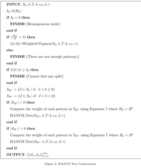
INPUT:S0,λ, T, k,ǫP,δ,τ I0=I(H0)
if I0= 0then
FINISH{Homogeneous node}
end if if (|S0|
N >δ)then
{w, b� }=Weighted-Pegasos(S0,λ, T, k,ǫP,τ)
else
FINISH{There are not enough patterns.}
end if
if I(w, b� )≥I0then
FINISH{Cannotfind any split}
end if
SHl ={�x∈S0|w�·�x+b≤0}
SHr ={�x∈S
0|w�·�x+b >0}
if |SHl|>0 then
Compute the weight of each pattern inSHl using Equation 7 whereHk=Hl
H-LSVM Tree(SHl,λ, T, k,ǫP,δ,τ)
end if
if |SHr|>0then
Compute the weight of each pattern inSHr using Equation 7 whereHk=Hr
H-LSVM Tree(SHr,λ, T, k,ǫP,δ,τ)
end if
OUTPUT: {(w�n, bn)}Nn=1H
Training Classification Linear SVM N dlog�1 ǫ � d SMO-SVM N2 ×d nSV×nK(d) H-LSVM NHkd λǫ N P H(�x)×d
Table 1: Number of operations needed to train a setSofNpatterns in ad-dimensional space (Trainingcolumn) and to classify
a new pattern (Classification column) by Linear SVM, SVM-SMO and the H-LSVM algorithm. λ: regularization parameter
in Pegasos formulation. ǫ: optimization tolerance. nSV: number of support vectors of the non-linear SVM model. nK(d):
operations are needed to compute the kernel between each support vector and the test pattern.NH: total number of internal
nodes in the H-LSVM tree. ni: number of training samples which reach the nodeiin the H-LSVM tree. NHP(�x): number of
nodes encountered by pattern�xin the H-LSVM tree.
Table 1 (columnTraining) shows the training time complexities of the three algorithms: linear SVM, 259
SVM-SMO and H-LSVM. The H-LSVM cost is highly dependent on each dataset as it is determined by 260
the structure of the tree (NH). As expected, the lowest training cost corresponds to the linear SVM. The
261
comparison between the training times of non-linear SVM and H-LSVM is not straightforward as it depends 262
on the H-LSVM tree structure and the λ andǫ parameters. H-LSVM would be faster than SMO-SVM in 263
the training phase if NHk
λǫ ≪N
2. 264
3.2. Prediction Complexity 265
The cost of classifying a new pattern�x∈Rd by a linear SVM is the cost of computing the dot product
266
between the model hyperplane and the pattern to be classified: O(d). In the case of non-linear SVMs, the 267
classification of the pattern�x is carried out according to: �nSV
i=1 αi×K(x�i,�x), nSV being the number of
268
support vectors. If nK(d) is the number of operations needed to compute K(x�i,�x), the SVM prediction
269
complexity isnSV×nK(d). The proposed H-LSVM algorithm needs tofind the leaf of the tree for the pattern
270
�
x which leads toNP
H(�x)×doperations,NHP(�x) being the number of internal nodes –oblique hyperplanes–
271
evaluated by the algorithm until the pattern�xreaches a leaf in the tree. 272
The summary of the number of operations needed by each algorithm to classify a new pattern�xis given 273
in Table 1 (columnClassification). 274
Obviously the lowest classification cost corresponds to the linear SVM but it will be shown in Section 5 275
that the linear model is not usually competitive enough for real-world datasets. As regards the non-linear 276
models, it is reasonable to assume that the number of kernel operations nK(d) is at leastd. In that case,
277
H-LSVM has the lowest cost if the number of node evaluations needed to classify the pattern�x,NP H(�x), is
278
lower than the number of support vector encountered by SVM, nSV. In Section 5, the values ofnSV and
279
NP
H(�x) for real-world datasets are given, and it is shown that, in practice, the number of evaluations needed
280
by H-LSVM is indeed several orders of magnitude lower. 281
4. Generalization Error Bound for the H-LSVM Algorithm
282
In this section we provide a generalization error bound for the H-LSVM algorithm. First, we show 283
that the H-LSVM learning algorithm always converges and produces a decision tree as a final model. The 284
number of nodes to be generated isfinite and upper bounded by the number of training samples because of 285
the stopping criteria commonly used in learning decision tree schemes: the tree expansion isfinished when 286
there is no improvement in the impurity measure or when there are not enough patterns in a node. The 287
convergence properties of the model can be obtained by considering each node separately and applying the 288
Pegasos convergence bounds [13] which hold in the weighted version. 289
The generalization error bound is obtained based on the results given by Golea et al. in [40]. Although 290
other bounds for decision trees have been proposed in the literature [41, 42], some of them tighter than 291
those of Golea et al., the latter has been considered in this paper because of its simplicity and its explicit 292
dependence on the decision tree parameters, favoring the understandability of the empirical results obtained 293
in Section 5.6. Among the alternative bounds, the work of Shah [42] based on the Sample Compression (SC) 294
paradigm deserves a special mention because it generally yields tighter bounds and sparse models. These 295
bounds assume axis-parallel decision trees and their application to H-LSVM trees is not straightforward. 296
The formulation of the SC bounds for oblique decision trees is a direction for future work which might 297
also help to alleviate (or even eliminate) the cost of the pruning phase by using these bounds to guide the 298
learning process in a similar way as in [42, 43, 44, 45]. 299
Suppose a two-class decision tree T whose internal decision nodes are labeled with boolean functions 300
from some classU and whose leaves are labeled as−1 or 1. The bounds obtained depend on the effective 301
number of leavesLeff, a data-dependent quantity which reflects how uniformly the training data covers the
302
tree’s leaves and which can be considerably smaller than the total number of leaves in the tree,L[46]. This 303
bound is different from the Vapnik−Chervonenkis one, which depends on the total number of leaves in the 304
tree [47, 48]. 305
Formally, let P = (P1, . . . , PL) the probability vector which represents the probability of a pattern �x
306
reaching leafifori= 1. . . L. Then, the quadratic distance between the probability vectorP and the uniform 307
probability vectorU = (1/L, . . . ,1/L) is given byρ(P, U) =�Li=1(Pi−1/L)2and the effective number of
308
leaves in the tree is defined byLeff≡L(1−ρ(P, U)).
309
A bound of misclassification probability under the distributionD,PD[T(�x)�=y], can be estimated using 310
the following theorem [40]: 311
Theorem 1. For a fixed ξ > 0, there is a constant c that satisfies the following. LetD be a distribution 312
onX× {−1,+1}. Consider the class of decision trees of a depth of up to D, with decision functions inU. 313
With a probability of at least1−ξ on the training setS (of sizeN), every decision treeT that is consistent 314
with S has 315
PD[T(�x)�=y]≤c �
LeffVCdim(U)log2N log D
N
�12
whereLeff is the effective number of leaves ofT andV Cdim is the Vapnik Dimension. 316
The H-LSVM algorithm is in line with this framework identifying the classU with the Linear SVM. It 317
is known that the Vapnik Dimension of a hyperplane in ad-dimensional space is (d+ 1) [49] therefore, the 318
error bound for the H-LSVM method is reformulated as, 319
Lemma 2. For a fixedξ >0, there is a constant c that satisfies the following. LetD be a distribution on 320
X× {−1,+1}. Consider the class of decision trees of a depth of up toD, with H-LSVM decision functions. 321
With a probability of at least1−ξ on the training setS (of sizeN), every decision treeT that is consistent 322 with S has 323 PD[T(�x)�=y]≤c � Leff(d+ 1)log2N log D N �12 (10) whereLeff is the effective number of leaves ofT.
324
In practice it is quite difficult to have a consistent tree with the training dataS. In that case, a bound 325
of the misclassification probability can be obtained as a function of the misclassification probability in S, 326
PS[T(�x)�=y]. Now, the probability vectorP is reformulated according to the training set as:
327
Pi′=
PiPS[T(x�) =y|�xreaches leafi] PS[T(�x) =y]
By applying the theorem given in [40] for the particular case of the H-LSVM tree, we obtain the following 328
result, 329
Lemma 3. For a fixed ξ > 0, there is a constant c that satisfies the following. Let D be a distribution 330
on X× {−1,+1}. Consider the class of decision trees of a depth of up to D with H-LSVM internal node 331
decision functions. With a probability of at least 1−ξ on the training setS (of sizeN), every decision tree 332 T has 333 PD[T(�x)�=y]≤PS[T(�x)�=y] +c � L′ eff(d+ 1)log2N log D N �13 (11) wherecis a universal constant, andL′
eff=L(1−ρ(P′, U))is the empirical effective number of leaves of 334
T. 335
Therefore, for a given training setSofN patterns, the parameters of the tree which determine the error 336
bound for the H-LSVM algorithm are the depthD of the tree and the effective number of leavesLeff: the
337
lower these parameters are, the better generalization error. The parameter values and an estimation of the 338
model complexity according to Equation 11 are given in Section 5. 339
5. Experiments
340
The aim of the experiments described in the following subsections is fourfold: 341
• Compare H-LSVM with linear SVMs and non-linear SVMs in terms of classification accuracy and 342
prediction complexity (Section 5.2). 343
• Compare H-LSVM with Zapi´en’s [21, 24] and Adaboost [50] algorithms in terms of classification 344
accuracy and prediction complexity (Sections 5.3 and 5.4). 345
• Analyze numerically the H-LSVM scalability (Section 5.5). 346
• Analyze numerically the H-LSVM error bound studied in Section 4 (Section 5.6). 347
The H-LSVM has been implemented in C language and the code can be found at: 348
https://sites.google.com/site/irenerodriguezlujan/HLSVM-1.1.zip. 349
As the H-LSVM algorithm has been designed for binary classification domains, the experiments have 350
been conducted in large-scale binary classification problems. We have considered the large-scale datasets 351
used by Keerthi et al. [2]: IJCNN, Shuttle,M3VO and Vehicle. TheShuttle dataset has been converted 352
to a binary classification problem by differentiating class 1 from the rest. In the same way, the Vehicle 353
dataset has been reformulated as a binary classification task consisting of differentiating class 3 from the 354
rest. TheM3VOdataset corresponds to differentiate digit 3 from all the other digits in theMNIST problem. 355
An extension of the MNIST dataset with 8,100,000 patterns (MNIST8m) has also been included since it 356
represents a very large-scale classification problem. Again, the classification of digit 3 from all of the others 357
has been considered (M3VOm8). In order to compare the performance of our method with the Zapi´en 358
algorithm [21, 24], initially we chose the binary datasets used in this work: Heart and Faces. However 359
in the case of the Heart dataset, the classification accuracy of the linear SVM is the same as that of the 360
non-linear SVM and thus, we decided not to include this dataset in our experiments. Finally, we added the 361
binary version of the covtype dataset (class 2 versus others) because of its large number of patterns. The 362
characteristics of the datasets are shown in Table 2 as well as the repositories where they are available. 363
In most of the datasets (IJCNN,Shuttle, M3VO and Vehicle), the training and test subsets are given 364
beforehand. In the Faces dataset, we followed the experimental setup described in [52] which uses two 365
# Train # Test # Feat. Repository IJCNN 49,990 91,701 22 LIBSVM [51] Shuttle 43,500 14,500 9 LIBSVM [51] M3VO 60,000 10,000 780 LIBSVM [51] M3VOm8 810,000 7,290,000 784 LIBSVM [51] Vehicle 78,823 19,705 100 LIBSVM [51] Faces 8,525 4,263 576 http://www.cs.ubc.ca/~pcarbo/#data
Binary Covtype 522,910 58,102 54 LIBSVM Reposity [51]
Table 2: Binary datasets used to compare H-LSVM with linear SVMs and non-linear SVMs.
thirds of the observations for the training and the rest as a testing set. Moreover, data was normalized to 366
minimum and maximum feature values. We run the experiments on 10 different randomly chosen training-367
test partitions of the dataset. In the case of the M3VOm8 and Covtype datasets, we have tried to use as 368
many training patterns as possible in order to simulate a large-scale system with a high number of support 369
vectors3. Then, thefirst 810,000 patterns in theM3VOm8 dataset were used for training and the remaining 370
samples for test. In the Covtype dataset, according to the experiments carried out in [9, 53], 9/10 of the 371
samples for training and the remaining patterns for test. In both cases, the experiments were run on 10 372
different randomly chosen training-test partitions of the dataset. 373
In all of the experiments, linear SVMs and non-linear SVMs implemented in LIBLINEAR [36] and 374
LIBSVM [51] packages were used. The Gaussian kernel, k(xi, xj) = exp �
−γ�xi−xj�2 �
, was used for 375
non-linear SVMs. 376
5.1. Hyperparameter Tuning 377
Linear SVMs, non-linear SVMs and H-LSVM need to determine the values of a few parameters. In all 378
datasets, except Covtype, the hyperparameter selection has been made using a 5-fold cross validation on 379
the training set. The cost parameters in linear SVMs and non-linear SVMs were selected from the grid 380
10i, i = −6, . . . ,6. The γ parameter of the Gaussian kernel was taken from the range 10i, i = −3, . . . ,3.
381
Finally, for the H-LSVM model, we fixed the maximum number of Pegasos iterations T = 107 with a 382
tolerance ofǫP = 10−4and the minimum proportion of patterns needed to split a nodeδ was chosen as 10−i
383
withi=⌊log10N⌋to guarantee that the H-LSVM grows to a sufficient size (pruning is applied if necessary). 384
The regularization parameterλwas chosen from the grid 10i
N , i=−6, . . . ,6,N being the number of training
385
3
LIBLINEAR LIBSVM H-LSVM c c γ λ ρ IJCNN 101 101 100 10−5 0 Shuttle 102 106 100 10−7 0.2 M3VO 100 102 10−2 10−4 0.2 M3VOm8 100 102 10−2 10−5 0.2 Vehicle 10−1 101 10−1 10−6 0.1 Faces 10−1 101 10−2 10−5 0.1 Covtype 100 100 0.346 10−7 0.0
Table 3: Parameters used in the linear SVM, non-linear SVM and H-LSVM models for each binary dataset.
samples. The grid was obtained from the equivalenceλ= CN1 between the LIBLINEAR and LIBSVM cost
386
parametercand theλregularizer in H-LSVM. The prune rateρtook values in [0.0,0.1,0.2]. For theCovtype 387
dataset, we used the non-linear SVM hyperparameters provided in [9]. The resulting parameters for each 388
dataset and each model are given in Table 3. 389
5.2. Results 390
The results in terms of classification error (Error (%)) and classification cost are shown in Table 4. In 391
the case of the linear SVM, the number of hyperplane evaluations is shown whereas the number of support 392
vectors is indicated for the non-linear SVM (nSV or Hyp). While the classification cost of linear/non-linear
393
SVMs is independent of the test sample, the H-LSVM prediction cost depends on the path of the pattern in 394
the H-LSVM tree. Thus, the mean number of H-LSVM hyperplanes encountered per test sample together 395
with the maximum number of H-LSVM hyperplane evaluations written in parentheses are shown. In those 396
cases in which there were several training/test partitions, the average and standard deviation on the 10 runs 397
of the experiment are shown. 398
The quantification of the performance of the algorithms considering the linear and non-linear SVMs as 399
the points of reference is given by the quantitiesRelative Error (RE) andRelative Complexity (RC), 400 RE = eLSVM−e eLSVM−eSVM (12) RC = Hyp−1 nSV −1 , (13)
wheree represents the classification error rate. A value equals 0 at these magnitudesRE/RC indicate 401
that the classification accuracy/complexity is the same as that of the linear SVM while a value of 1 represents 402
the equivalence with the non-linear case. Therefore, it would be desirable to have a Relative Error close to 403
1 and aRelative Complexity close to 0. 404
As expected, the classification results of the non-linear SVMs are greater than those of the linear SVM 405
and H-LSVM. However, the classification accuracy of the H-LSVM is significantly better than that of the 406
linear model in all cases. These results are not surprising because the proposed H-LSVM method is simpler 407
than the non-linear SVM but more sophisticated than linear SVMs. While the classification error of H-408
LSVM is closer to that of the non-linear SVM in most cases, the H-LSVM classification accuracy is closer 409
to the linear model for the Faces and M3VO datasets. Nevertheless, in the case of theFaces dataset the 410
H-LSVM model represents an improvement of 41% in respect to the linear SVM and it will be shown later 411
that it yields significantly better results than the Zapi´en et al. [21] algorithm. These results show that the 412
non-linear SVMs cannot be approximated by the proposed method in certain domains. It is worth pointing 413
out that H-LSVM outperforms the non-linear SVM in the Covtype dataset. Although, the classification 414
error obtained for the non-linear SVM is comparable to the results reported in [9], a thorough search of 415
the non-linear SVM parameters might provide better results. Unfortunately, to apply the hyperparameter 416
procedure described in Section 5.1 is unfeasible because of the size of the dataset and the number of support 417
vectors. 418
Our main interest is not having the best classification error rates but providing a method capable of 419
classifying a pattern in few milliseconds while obtaining a competitive performance. In this respect, the 420
non-linear SVM needs the largest number of operations in prediction while the lowest cost is that of the 421
linear SVM. However, the performance of the linear SVM can be extremely poor as in theIJCNN orCovtype 422
datasets. The classification complexity of H-LSVM is between these two models: it is higher than that of the 423
linear SVM –in the worst case it increases the cost of the linear model in one order of magnitude– but much 424
lower than the cost of the non-linear SVM –H-LSVM can accelerate the prediction cost of the non-linear 425
SVM even by a factor of 104 as in the case of the M3VOm8 and Covtype datasets. In fact, the Relative 426
Complexity is lower than 10−1in all cases. 427
5.3. Results: Comparison with SVM Trees Algorithm 428
Having compared H-LSVM to baseline models, we can contrast the results with the Zapi´en decision 429
tree [21]. As mentioned above, only one of the two binary classification problems used in this work cannot 430
be classified accurately by a linear SVM (Faces). Despite the fact that our method has been designed for 431
binary classification problems, the performance of our model in the multiclass USPS dataset was measured. 432
The USPS dataset for handwritten text recognition is available in the LIBSVM Repository [51]. It consists 433
of 7291 training samples and 2007 test samples. Each example is described by 256 features. Following 434
the methodology described in [52], we normalized the data to minimum and maximum feature values and 435
we applied one against one approach (1A1) for the multiclass problem. The 1A1 strategy consists of 436
IJCNN Linear SVM Non-linear SVM H-LSVM Class. Err (%) 7.82 1.01 2.36 nSV or Hyp 1 3,154 7.28 (16) RE / RC 0 / 0 1 / 1 0.80 / 2.0·10−3 Shuttle Linear SVM Non-linear SVM H-LSVM Class. Err (%) 2.21 0.062 0.10 nSV or Hyp 1 66 5.18 (12) RE / RC 0 / 0 1 / 1 0.98 / 6.43·10−2 M3VO Linear SVM Non-linear SVM H-LSVM Class. Err (%) 2.09 0.33 1.79 nSV or Hyp 1 2,873 3.15 (8) RE / RC 0 / 0 1 / 1 0.17 / 7.49·10−4 M3VOm8 Linear SVM Non-linear SVM H-LSVM Class. Err (%) 3.90 0.03 1.43±0.02 nSV or Hyp 1 13,471 4.73±0.003 (11.00±0.00) RE / RC 0 / 0 1 / 1 0.64 / 2.77·10−4 Vehicle Linear SVM Non-linear SVM H-LSVM Class. Err (%) 14.18 11.88 12.61 nSV or Hyp 1 23,642 2.84 (10) RE / RC 0 / 0 1 / 1 0.68 / 7.78·10−5 Faces Linear SVM Non-linear SVM H-LSVM Class. Err (%) 8.81±0.35 2.97±0.24 6.39±0.43 nSV or Hyp 1 1,260.3±14.81 2.59±0.06 (5.30±0.15) RE / RC 0 / 0 1 / 1 0.41 / 1.26·10−3 Covtype Linear SVM Non-linear SVM H-LSVM Class. Err (%) 23.66±0.21 18.57±0.20 11.39±0.08 nSV or Hyp 1 245,687.2±167.8 12.93±0.087 (44.00±1.08) RE / RC 0 / 0 1 / 1 2.41 / 4.86·10−5
Table 4: Test error rate (Class. Err (%)) and classification complexity (nSV or Hyp) of Linear SVMs, non-linear SVMs
and H-LSVM. The mean number of hyperplane evaluations per test sample is indicated for linear SVMs and H-LSVM. The maximum number of H-LSVM hyperplane evaluations is shown in parentheses. In the case of non-linear SVMs, the number of
Faces
Linear SVM Non-linear SVM SVM Trees H-LSVM
Class. Err (%) 8.81 2.97 8.99 6.39
nSV or Hyp 1 1260.3 4 2.59 (5.30)
RE / RC 0 / 0 1 / 1 −0.03 / 0.002 0.41 / 0.001
USPS
Linear SVM Non-linear SVM SVM Trees H-LSVM
Class. Err (%) 8.67 4.53 6.24 5.38
nSV or Hyp 1 1521 49 64.77 (117)
RE / RC 0 / 0 1 / 1 0.59 / 0.03 0.79 / 0.04
Table 5: Comparison of the SVM Trees method by Zapi´en et al. [21, 52] and H-LSVM. Misclassification error (Class. Err
(%)) and the mean number of hyperplane evaluations per test sample (Hyp) are shown for both methods and for the linear and
non-linear SVMs (nSV). The maximum number of H-LSVM hyperplane evaluations is indicated in parentheses. The number
of hyperparameter evaluations was computed as the sum of the hyperplanes evaluated in every binary classifier. TheRelative
Error (RE)and theRelative Complexity (RC)of the SVM Trees method and H-LSVM are also given.
training a classifier for every pair of classes and classifying a new pattern based on majority voting. The 437
hyperparameters were chosen by using 5-CV as described above. For the linear SVM, the cost parameter 438
was set to c= 1, for the non-linear SVMc= 101 and γ= 10−2 and for the H-LSVM algorithmλ= 10−5 439
and ρ= 0. The results in terms of the misclassification error and classification cost for both methods are 440
given in Table 5. The performance of the Zapi´en method has been extracted from [21, 52]. 441
In both cases H-LSVM is superior in terms of classification accuracy whereas the classification cost is in 442
the same order of magnitude. Specifically, their classification complexity is quite similar in theFacesdataset 443
but the SVM Trees algorithm is slightly faster for theUSPS database. In any case, the classification cost of 444
both algorithms is of the same order of magnitude. In summary, the H-LSVM decision tree, expanding both 445
children of each node as well as the weighted patterns used in the linear SVM training, provide advantages 446
in terms of classification accuracy while maintaining the classification cost. It is also worth noting that in all 447
cases the maximum depth of the tree is lower than the number of internal nodes (the number of linear SVMs), 448
which means that the structure of the tree is far from being a cascade of classifiers as in [21, 24, 25, 52]. 449
The superiority of the H-LSVM tree against the Zapi´en’s algorithm in terms of classification accuracy is not 450
surprising given that, as already mentioned in Section 1, the hypothesis class of H-LSVM (disjunctions of 451
conjunctions) is more general than that of the SVM Trees algorithm (conjunctions) [22]. What is more, this 452
difference can be quantified taking into account that the number of decision tree skeletons withkdecision 453
1000 101 102 103 104 105 106 5 10 15 20 25 nSV / Hyp
Classification Error Rate (%)
IJCNN Shuttle M3VO M3VOm8 Vehicle Faces Binary Covtype USPS
Figure 4: Best viewed in color. Classification complexity (nSV / Hyp) versus classification error rate for different datasets.•
Linear SVM�Non-linear SVM�H-LSVM.
nodes is given by thek-th Catalan Number [19, 23] in comparison to the only one possibility for the Zapi´en’s 454
method. 455
In order to visualize the trade-offbetween the misclassification error vs. classification cost, Figure 4 shows 456
the dependence between these two magnitudes for the linear SVM, non-linear SVM and H-LSVM. The x-457
axis represents the number of support vectors or hyperplanes encountered by each method in logarithmic 458
scale. The y-axis shows the classification error rate. Each dataset is represented by a color according to 459
the legend. Circles, squares and diamonds represent the linear SVM, non-linear SVM and H-LSVM models, 460
respectively. The lower left-hand area is associated to the best scenario: the lowest classification error 461
and the lowest classification complexity. In this Figure, three clusters can be easily identified according to 462
the classifier (circles, squares and diamonds). Clearly, the non-linear SVMs have the highest classification 463
complexity while the H-LSVM cost is closer to the linear one. Looking at the classification error, in all cases 464
the non-linear SVM is superior – except theCovtypedataset – and the H-LSVM effectiveness is greater than 465
that of the linear model. 466
Finally, to give an idea of the quality of the H-LSVM algorithm with regard to the prediction time, 467
Table 6 shows the time in seconds needed by a linear SVM, a non-linear SVM and H-LSVM to classify 468
a new pattern in an Intel(R) Core(TM) i7 CPU 920 at 2.67GHz. The training time is also included for 469
completeness. As expected, the lowest training and test times correspond to the linear SVM. As regards the 470
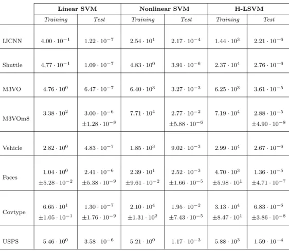
Linear SVM Nonlinear SVM H-LSVM
Training Test Training Test Training Test
IJCNN 4.00·10−1 1.22·10−7 2.54·101 2.17·10−4 1.44·103 2.21·10−6 Shuttle 4.77·10−1 1.09·10−7 4.83·100 3.91·10−6 2.37·104 2.76·10−6 M3VO 4.76·100 6.47·10−7 6.40·103 3.27·10−3 6.25·103 3.61·10−5 M3VOm8 3.38 ·102 3.00·10−6 7.71·104 2.77·10−2 7.19·104 2.88·10−5 ±1.28·10−8 ± 5.88·10−6 ± 4.90·10−8 Vehicle 2.82·100 4.83·10−7 1.85·103 9.02·10−3 2.99·104 2.67·10−6 Faces 1.04 ·100 2.41·10−6 2.39·101 2.52·10−3 4.70·103 1.36·10−5 ±5.28·10−2 ± 5.38·10−9 ± 9.61·10−2 ± 1.66·10−5 ± 5.98·101 ± 4.71·10−7 Covtype 6.65 ·101 1.30·10−7 2.10·104 1.95·10−2 3.13·104 6.83·10−6 ±1.05·10−1 ± 1.76·10−9 ± 1.31·102 ± 7.43·10−5 ± 8.47·101 ± 3.86·10−8 USPS 5.46·100 3.58·10−6 5.21·100 1.17·10−3 5.88·103 1.59·10−4
Table 6: Training and testing time in seconds required by LIBLINEAR, LIBSVM and H-LSVM.
training cost discussed in Section 3.1, the differences between the training cost of the non-linear SVM and 471
H-LSVM are given by the structure of the H-LSVM tree. Therefore, depending on the dataset either the 472
linear SVM or H-LSVM is faster in the training phase. Focusing on the aim of speeding up the non-473
linear SVM prediction cost, the H-LSVM classification time is always in the order of tenths of milliseconds 474
at most and significantly lower than those of the non-linear SVM. 475
476
Several techniques based on the use of linear SVMs on the manifold coordinates have come out recently 477
[15, 16, 17]. In particular, the Locally Linear SVM (LLSVM) model proposed by Ladicky et al. [17] reports 478
results for the USPS dataset. The classification accuracy of H-LSVM is slightly better than that of the 479
LLSVM and the LLSVM algorithm needs to compute the distance to 100 k-means centroids while H-LSVM 480
evaluates on average 64.77 hyperplanes (maximum 117). That is, both methods are comparable in terms of 481
classification accuracy and prediction complexity. 482
5.4. Results: Comparison with Adaboost Algorithm 483
Other natural competitors for H-LSVM are boosting algorithms [54] since they create piecewise linear 484
functions with a good generalization performance [55] and low classification cost. In particular, we have 485
considered the most known boosting algorithm: AdaBoost (Adaptive Boosting) [50]. Decision stumps were 486
used in accordance with the Adaboost algorithm originally proposed by its authors Freund and Schapire 487
[50] and motivated by its successful application in the state-of-the-art Viola-Jones face detection algorithm 488
[56]. The main advantage of Adaboost with decision stumps on competitors is the speed of learning and 489
prediction, which is particularly critical in large-scale problems. 490
Adaboost requires the establishment of the maximum number of weak classifiersH to be used. Since our 491
paper focuses on accelerating the classification times,H wasfixed to make the prediction cost of Adaboost 492
comparable to that of H-LSVM. Then, by taking into account that Adaboost needs to evaluate all the weak 493
learners to classify a test pattern and considering that the prediction complexity of each decision stump is 494
O(1),His computed as the mean number of hyperplanes evaluated by H-LSVM multiplied by the dimension 495
of the patterns. The comparison of both methods in terms of misclassification rate and classification cost 496
as well as the value of the parameterH for each dataset are given in Table 7. 497
The results show that Adaboost has a better performance in theShuttleandVehicledatasets, the diff er-498
ence in classification accuracy being 0.15% at most. However, in some cases such asIJCNN and Covtype, 499
H-LSVM significantly outperforms Adaboost. On average, Adaboost and H-LSVM have misclassification 500
rates of 7.81% and 5.15%, respectively on all the datasets. Overall, the H-LSVM yields a better perfor-501
mance/classification speed ratio than Adaboost with decision stumps. 502
5.5. Numerical Analysis of H-LSVM Scalability 503
To illustrate the applicability of the H-LSVM algorithm to real large-scale scenarios, we show the scala-504
bility in the training time and convergence of the test error rates as the number of training samples increases. 505
In this regard, Figures 5a – 5c show the training complexity of H-LSVM in terms of the number of hyper-506
planes in the H-LSVM tree and the computational time as a function of the number of training samplesN. 507
Figure 5d shows the training and test classification accuracies as a function ofN. The results represent the 508
average on the 10 training/test partitions of theBinary Covtype dataset. In turn, 4 subsets of size 10,000, 509
50,000, 100,000 and 200,000, respectively, have been randomly chosen from each training partition. 510
According to the training cost of H-LSVM presented in Section 3.1,O(NHkd
λǫ ), by maintainingλ,ǫandd
511
constant for the different training sizes, the training cost of H-LSVM depends on the subsampling ratekand 512
the number of internal nodes in the H-LSVM treeNHasO(NHk). Unfortunately,NH depends inextricably
513
on the problem in question and thus, a general estimation ofNHbased onN cannot be provided. However,
514
it is possible to compare the number of internal nodes in the H-LSVM tree against those corresponding to 515
the best tree (balanced tree) and the worst one (a linear or cascade tree). In this regard, Figures 5a (linear 516
Adaboost H-LSVM
Class. Err (%) H Cost Class. Err (%) Hyp Cost
IJCNN 6.50 170 170 2.36 7.28 160.16 Shuttle 0.08 50 50 0.10 5.18 46.62 M3VO 2.69 2460 2460 1.79 3.15 2457.00 M3VOm8 3.61±0.01 3710 3710 1.43±0.02 4.73 3708.32 Vehicle 12.46 290 290 12.61 2.84 284.00 Faces 6.39±0.33 1500 1500 6.39±0.43 2.59 1491.84 Binary Covtype 22.95±0.23 700 700 11.39±0.08 12.93 698.22 Average 7.81 1268.57 1268.57 5.15 5.53 1263.74
Table 7: Test error rate (Class. Err (%)) and classification complexity (Cost) of Adaboost and H-LSVM. The number of
weak learners (H) are indicated for Adaboost and the mean number of hyperplane evaluations per test sample is indicated for
H-LSVM (Hyp). Note that the classification cost is computed by considering that the classification complexity of each decision
0 1 2 3 4 5 x 10⁵ 0 1 2 3 4 5x 10 5
Number of training samples (N)
Number of internal nodes (N
H ) (a) H−LSVM tree Balanced tree Linear tree 0 1 2 3 4 5 x 10⁵ 100 102 104 106
Number of training samples (N)
Number of internal nodes (N
H ) (b) H−LSVM tree Balanced tree Linear tree 0 1 2 3 4 5 x 10⁵ 0 1 2 3 4x 10⁴
Number of training samples (N)
Training time (seconds)
(c) H−LSVM 0 1 2 3 4 5 x 10⁵ 75 80 85 90 95
Number of training samples (N)
Classification accuracy (%)
(d)
H−LSVM training H−LSVM test
Figure 5: H-LSVM training complexity and classification rate convergence as a function of the number of training samples (N)
for theCovtypedataset. Figure 5a: number of internal nodesNHin the H-LSVM tree. Reference values corresponding to a
balanced and cascade tree are also included. Figure 5b: Figure 5a using logarithmic axis in the y-axis. Figure 5c: training time of the H-LSVM algorithm. Figure 5d: training and test classification accuracies.
y-axis) and 5b (logarithmic y-axis) include the number of internal nodes associated with the balanced 517
decision tree (log2(N)) and those encountered in the cascade structure (N). In this case, the complexity of 518
the H-LSVM tree is closer to that of the balanced tree. Similar results are expected for the other datasets 519
since in all cases the maximum depth of the tree is much lower than the number of internal nodes. 520
Furthermore, the variability in the distribution of the training samples throughout the decision tree also 521
affects the exact computation of a general training cost of the Pegasos algorithm in each node. Although 522
the subsample size kis fixed at the beginning of the algorithm – in this experiment, it was set 50,000 –, 523
the effective subsampling size in each node is determined online as the minimum betweenkand the number 524
of samples reaching the current node, which is totally linked to each particular dataset. Nevertheless, the 525
empirical measure of the training time of H-LSVM as a function of the number of training samplesNshown 526
in Figure 5c seems to have a linear growth and, in fact, it has been proven that the polynomial curvefitting 527
the points with the lowest error is that of degree 1. Again, a comparison with the training complexity of the 528
balanced and the linear decision trees can be valuable. Under the assumption that the cost of computing 529
the split of the i-th node is proportional to the number of samplesni reaching the node, the balanced tree
530
has a linear cost with respect toN: 531 log2(N) � i=0 i ni= log2(N) � i=0 i i 2i =O(N),
while the linear tree has a quadratic dependence: 532 N−1 � i=0 ni= N−1 � i=0 (N−i) =O(N2).
Therefore, the complexity of H-LSVM training is closer to the best scenario. Finally, Figure 5d reveals 533
that the gap between training and test errors converges with approximately 300,000 patterns. Although 534
the classification accuracy in the test set increases with the number of training samples, the improvement 535
becomes smaller as N grows, especially when N is larger than 300,000 in which case the difference with 536
respect to the model trained with all the training samples is 0.52%. 537
The preceding results corroborate the applicability of H-LSVM to large-scale scenarios. 538
5.6. Numerical Analysis of H-LSVM Generalization Error Bound 539
Lemma 3 provides a generalization error bound for the H-LSVM method as a function of some data-540
dependent parameters according to the equation, 541 PD[T(�x)�=y]≤PS[T(�x)�=y] +c � L′ eff(d+ 1)log2N log D N �13


![Table 5: Comparison of the SVM Trees method by Zapi´ en et al. [21, 52] and H-LSVM. Misclassification error (Class](https://thumb-us.123doks.com/thumbv2/123dok_us/9716422.2853221/22.892.169.707.162.274/table-comparison-trees-method-zapi-lsvm-misclassification-class.webp)