Programming
P. A. M. Casares1,∗ and M. A. Martin-Delgado1,† 1Departamento de F´ısica Te´orica, Universidad Complutense de Madrid.
(Dated: July 7, 2020)
We introduce a new quantum optimization algorithm for dense Linear Programming problems, which can be seen as the quantization of the Interior Point Predictor-Corrector algorithm [1] using a Quantum Linear System Algorithm [2]. The (worst case) work complexity of our method is, up to polylogarithmic factors, O(L√n(n+m)||M||F¯κ−2) forn the number of variables in the cost function,mthe number of constraints,−1 the target precision,Lthe bit length of the input data, ||M||F an upper bound to the Frobenius norm of the linear systems of equations that appear,||M||F, and ¯κan upper bound to the condition numberκof those systems of equations. This represents a quantum speed-up in the numbernof variables in the cost function with respect to the comparable classical Interior Point algorithms when the initial matrix of the problemAis dense: if we substitute the quantum part of the algorithm by classical algorithms such as Conjugate Gradient Descent, that would mean the whole algorithm has complexityO(L√n(n+m)2κ¯log(−1)), or with exact methods, at leastO(L√n(n+m)2.373). Also, in contrast with any Quantum Linear System Algorithm, the algorithm described in this article outputs a classical description of the solution vector, and the value of the optimal solution.
Keywords: Linear Programming Problem, Quantum Algorithms, Quantum Linear Approximation, Interior Point Method, Iteration Complexity, Strong Polynomiality.
I. INTRODUCTION
Linear Programming problems are among the most fundamental optimization problems [3–5]. Ap-plications abound both at personal and professional fronts: improving a project delivery, scheduling of tasks, analyzing supply chain operations, shelf space optimization, designing better strategies and logis-tics and scheduling problems in general. Linear Pro-gramming is also used in Machine Learning where Supervised Learning works on the basis of linear programming. A system is trained to fit a math-ematical model of an objective (cost) function from the labeled input data that later can predict val-ues from unknown test data [6, 7]. More specifically, linear programming is a method to find the best out-come from a linear function, such as maximum profit or lowest cost, in a mathematical model whose re-quirements are represented by linear constraints of the variables. Semi-Definite Programming (SDP) is an extension of Linear Programming where the ob-jective or cost function is formulated with a non-diagonal matrix and constraints contain more gen-eral inequalities [8–11].
We are in the time of small quantum computers with reduced computational capabilities due to noisy physical qubits [12–15]. The challenge of surpassing the power of current and foreseeable classical
com-∗[email protected] †[email protected]
puters is attracting a lot of attention in the academia [16, 17] and in technological companies. This moti-vates the endeavour of searching for new quantum algorithms beyond the standard ones that spurred the field of quantum computation in the mid 90s (Shor, Grover, etc.) [18–21]. Only recently, a quan-tum algorithm for solving SDP problems has been proposed by Brand˜ao and Svore providing us with the first quantum advantage for these optimization problems [22–26].
A. Background on Linear Programming.
The development of methods to solve Linear Pro-gramming problems has a long tradition starting with the Simplex Method [5], which is simple and widely used in practice, but has (in the worst case) exponential time complexity in the number of vari-ables. In 1979 Khachiyan proved that the ellip-soid method ensured (weak) polynomial complexity the number of variables, O(n6L) [27]. However, in practice the ellipsoid algorithm is complicated and not competitive. In 1984 Karamark proposed the first Interior Point algorithm [28], with complexity O(n3.5L). It was more practical than the ellipsoid method and gave rise to a large variety of available Interior Point methods [29]. The best advantage of these methods is that, contrary to what happens in the Simplex Method, Interior Point algorithms have a worst case runtime polynomial in the number of variables. Among them, the Predictor-Corrector
Method [1, 30] is arguably one of the best proce-dures to achieve an extremely well-behaved solution, and requires just O(√nL) iterations. However, the Predictor-Corrector method does not explicitly indi-cate what method should be used to solve the linear system of equations that appear in each iteration, so the solution of the system will depend on what method is used, as can be seen in table I. For fur-ther background on Interior Point methods we refer the reader to the review [29].
B. Our algorithm
Here we present a quantum algorithm that re-lies on the quantization of this method. One im-portant feature of our quantum Interior Point algo-rithm is that it is a hybrid algoalgo-rithm: partially clas-sical, partially quantum. This feature has become very common and a similar situation occurs with the Brand˜ao-Svore algorithm in SDP, the Quantum Eigen-Solver for quantum chemistry [37–41], and many others, and has the advantage of requiring shorter coherence times. The core of the quanti-zation of the Interior Point algorithm relies on the use of the block encoding techniques [2], that extend the applicability of the Quantum Linear System Al-gorithm proposed by Harrow, Hassadim and Lloyd (HHL) [42] in the case where A is dense, to solve the linear system of equations that appear in the Predictor-Corrector steps.
However, in order to apply the QLSA in the con-text of Linear Programming, we have to solve several caveats since the straightforward application of it is doomed to failure.
The quantum Interior Point algorithm we pro-pose benefits from several fundamental properties inherited from the classical Predictor-Corrector al-gorithm, and has a better performance than other classical Interior Point algorithms. In particular [1]: 1. The Predictor-Corrector method can solve the Linear Programming problem without assum-ing the existence of feasible or optimal solu-tions.
2. If the Linear Programming problem has solu-tion, the loop of this interior point algorithm approaches feasibility and optimality at the same time for both the primal and dual prob-lem, and if the problem is infeasible or un-bounded the algorithm detects infeasibility for either the primal or dual problem.
3. The algorithm can start from any point near the center of the positive orthant.
The notions of feasible, optimal solutions etc. are defined in Sec. II where a self-contained review of the Predictor-Corrector method is presented.
The work complexity of the algorithm proposed here is O(L√n(n+m)||M||Fκ¯ −2), where n is the number of variables of the cost function, m is the number of constraints,L is the bit length of the in-put data (see Eq. (1)), ||M||F is an upper bound to the Frobenius norm of the linear systems of equa-tions that appear, ¯κis an upper bound to the con-dition numbers of the linear systems of equations that appear in the Predictor-Corrector steps, and −1 is the precision with which one wants to solve the linear system of equations. To avoid confusion notice that in the text we will callthe error and−1 its associated precision, because a low error means high precision and viceversa. The time complexity of the proposed quantum Interior Point algorithm can be reduced fromO(L√n(n+m)||M||Fκ¯ −2) to O(L√n||M||Fκ¯) distributing the work of each itera-tion between O((n+m)−2) quantum processors.
If we substituted the QLSA by a classical Linear System Algorithm, the price to pay would be, at least, an O(√n+m) increase in the work complex-ity, as ||M||F =O(
√
n+m) if the spectral norm of M is bounded [43]. For example, if we used con-jugate gradient descent, the overall algorithm com-plexity would beO(L√n(n+m)2κ¯log(−1)). Also, if we wanted to use an exact Linear System Algorithm the best we could hope for is the complexity it takes to exactly invert a matrix [33],O((n+m)2.373) [44], thus implying an overall work complexity for the al-gorithm O(√n(n+m)2.373L), that could be paral-lelized in (n+m)2.373 processors to lower the time complexity O(√nL) up to polylogarithmic terms [33]. A summary of these results is presented in table I.
It is worth mentioning that our quantization ap-proach to Linear Programming problems is radically different from the method of Brand˜ao and Svore and this comes with several benefits. Namely, the prob-lem of quantising linear programming using multi-plicative weight methods [45] as in Brand˜ao-Svore is that they yield an efficiency depending on parame-ters R and r of the primal and dual problems. In fact, these parameters might depend on the sizes n, mof the cost function, thereby the real time com-plexity of the algorithm remains hidden. For in-stance, for some classes of problems Rr/ = O(n) according to theorem 24 of [26]. Moreover and gener-ically, unless specified, theseR, rparameters cannot be computed beforehand, but after running the al-gorithm (we will have a similar situation with ¯κ). Thus, the real efficiency of the quantum algorithm is masqueraded by overhead factors behaving badly onRandr. Their algorithm has nevertheless a good
Algorithms for Linear Programming Work complexity Parallelizable? Pred-Corr. [1] + Conjugate Gradient [31] O(L√n(n+m)2κ¯log(−1)) O((n+m)2) Pred-Corr. [1] + Cholesky decomposition [32] O(L√n(n+m)3) O((n+m)2) Pred-Corr. [1] + Optimal exact [33] O(L√n(n+m)2.373) O((n+m)2.373) Multiplicative weights [25] O((√n Rr
+√m) Rr 4
) O(1)
Quantum Interior Point with Newton system [34] O(L√n(n+m)µ¯κ3−2log(0−1)) O((n+m)−2) Pred-Corr. [1] + Block-encoding [2] (This algorithm) O(L√n(n+m)||M||F¯κ−2) O((n+m)−2) TABLE I. Comparison of complexity of different algorithmsathat can be used for solving dense Linear Programming problems; the first three are purely classical whereas the following three are hybrid quantum-classical. It includes only leading-order terms. QLSA stands for a dense Quantum Linear System Algorithm [2]. Note that the algorithms [25] and [34] can be applied to more general problems concerning Semidefinite Programming. In the table µ ≤ ||M||F =O(√n), which reflects the fact that both [34] and our algorithm share common features even if they were developed independently. In reference [26], theorem 24, it is proven that for many combinatorial problems the term (Rr/) = O(n+m), affecting the complexity of [25]. With respect to L, for many cases the complexity of the Predictor-Corrector method does not depend onL [36]; but as an upper bound O(L) complexity will be common to all Interior Point methods [29]. In contrast, the Multiplicative weight method will not depend on it. Finally, the column ‘Parallelizable?’ gives the number of quantum or classical processors that can be used in parallel to solve the problem; the time complexity is divided by the corresponding amount.
a For completitude we want to mention that recently [35] has proposed quantum subroutines to speedup the simplex method.
complexity onn,O(√n+m), but much worse com-plexity on the precision,O(−5) for the most recent improvement of the Brand˜ao-Svore algorithm [25].
C. Structure of the paper
The paper has two main sections. The first re-views the Predictor-Corrector algorithm from [1]. It is itself divided in subsections where we explain how to initialize and terminate the algorithm, and the main loop.
In the second section we explain the changes we carry out to be able to use the QLSA from [2]. In particular we start with a subsection discussing the condition number and then we focus on how to pre-pare the initial quantum states for the QLSA and read out the results using a tomography protocol from [46]. Finally we explain the QLSA, comment on the possibility of quantizing the termination of the algorithm, and devote two subsections to the complexity of the overall algorithm and its compar-ison with other alternatives, and the possibility of failure.
We recommend the reader to first understand the Predictor-Corrector algorithm in its classical form, and then take a look at figures 1 and 2 in order to get an overall impression of the algorithm before trying to understand the technical details.
II. THE PREDICTOR-CORRECTOR
ALGORITHM
In this section we review the Predictor-Corrector algorithm of Mizuno, Todd and Ye for solving Linear Programming problems [1]. As stated in the original article, we will see that it performs O(√nL) itera-tions of the main loop in the worst case scenario, wherenis the number of variables andLthe size of the encoding the input data in bits:
L:= n X i m X j dlog2(|aij|+ 1) + 1e, (1)
foraij elements of the matrix defining the problem, A, that is defined in the following equations (2) and (3). Note that L =O(mn). However, in a typical case the number of iterations will not depend on L, but will rather beO(√nlogn) [36].
The linear programming problem we want to solve is called primal problem (Linear Problem, LP): Given A∈Rm×n,c∈
Rn andb∈Rm, findx∈Rn
such that:
minimizescTx (2a)
subject toAx≥b, x≥0. (2b) The dual problem (Dual Problem, DP) has the same solution: finding y∈Rmsuch that
maximizesbTy (3a)
Then, for linear programming problems, the primal-dual gap is 0:
bTy−cTx= 0. (4) A usual strategy is to use slack variables to turn all inequality constraints into equality constraints, at the cost of additional constraints. Thus, we can substitute ATy ≤cby ATy+s= c, s≥ 0∈
Rn
being the slack (dual) variable to the constraint (3).
A. Initialization
According to the prescription of [1], one way to solve the previous problems (2) and (3) is to set an-other problem from which the solution of (2) and (3) can be easily obtained. This new problem is homo-geneous, in the sense that there is a single non-zero constraint, and self-dual, as its dual problem is it-self. Therefore, letx0 >0∈Rn,s0 >0∈Rn, and
y0 ∈
Rm be arbitrary initialization variables which
will be chosen later on. Then, formulate the Homo-geneous Linear Problem (HLP) as
minθ (5) such that (x≥0, τ ≥0, τ ∈R): +Ax −bτ +¯bθ = 0 −ATy +cτ −c¯θ ≥ 0 +bTy −cTx +¯z θ ≥ 0 −¯bTy +¯cTx −z τ¯ = −(x0)Ts0−1 (6) with ¯ b:=b−Ax0, c¯:=c−ATy0−s0, ¯ z:=cTx0+ 1−bTy0. (7) The last constraint from (6) is used to impose self-duality. It is also important to remark that ¯b, ¯cand ¯
z indicate the infeasibility of the initial primal and dual points, and the dual gap, respectively.
Recall also that we use slack variables to con-vert inequality constraints into equality constraints. Those slack variables indicate the amount by which the original constraint deviates from an equality. As we have two inequality constraints, we introduce slack variabless ∈ Rn for the second constraint in
(6) andk∈R(in [1] denoted κ) for the third:
−ATy+cτ−c¯θ−s=0; s≥0 (8) bTy−cTx+ ¯zθ−k= 0; k≥0 (9) This implies that we can rewrite the last con-straint in (6) as
(s0)Tx+(x0)Ts+τ+k−((x0)Ts0+1)θ= (x0)Ts0+1. (10)
Once we have defined these variables, theorem 2 of [1] proves that any point fulfilling
y=y0, x=x0>0, s=s0>0, τ =k=θ= 1. (11) is a feasible point, and therefore a suitable set of initialization parameters for our algorithm. A par-ticularly simple one can choose is
y0= 0m×1, x0= 1n×1=s0, (12) where 1n×1= [1, ...,1]T, and 0m×1= [0, ...,0]T.
B. Main loop
In this section we explain how to set up an itera-tive method that allows us to get close to the opti-mal point, following a path along the interior of the feasible region. The original references are [1, 30]. Begin defining X := diag(x) and S := diag(s). Define also Fh the set of feasible points of (HLP) v = (y,x, τ, θ,s, k); and F0
h ⊂ Fh those such that (x, τ,s, k)>0.
Finally, define the following central path in (HLP)
C={(y,x, τ, θ,s, k)∈ F0 h: Xs τ k =x Ts+τ k n+ 1 1(n+1)×1}, (13)
and its neighbourhood
N(β) ={(y,x, τ, θ,s, k)∈ F0 h: Xs τ k −µ1(n+1)×1 ≤βµ whereµ= x Ts+τ k n+ 1 }. (14) Then, theorem 5 of [1] ensures that the central path lies in the feasibility region of (HLP).
In consequence, the algorithm proceeds as fol-lows: start from an interior feasible point v0 = (y0,x0, τ0, θ0,s0, k0)∈ F0
h. Then, recursively, form the following system of equations for variablesdv= (dy,dx, dτ, dθ,ds, dk) andt= 0,1, ...∈N: +A −b +¯b −AT +c −c¯ −1 +bT −cT +¯z −1 −¯bT +¯cT −z¯ dy dx dτ dθ ds dk = 0 0 0 0 (15a) Xtds+Stdx τtdk+ktdτ =γtµt1(n+1)×1− Xtst τtkt , (15b)
whereγttakes values 0 and 1 for even and odd steps respectively, starting int= 0. The linear system of
equations can be written in matrix form asMtdvt=
ft, i.e. m n 1 1 n 1 m 0 A −b b¯ 0 0 n −AT 0 c −c¯ −1 0 1 bT −cT 0 z¯ 0 −1 1 −¯bT c¯T −z¯ 0 0 0 n 0 St 0 0 Xt 0 1 0 0 kt 0 0 τt dy dx dτ dθ ds dk = 0 0 0 0 γtµt1 n×1−Xtst γtµt−τtkt . (16)
So, the main loop of the algorithm consists in per-forming the following steps iteratively:
Predictor step: Solve (16) with γt = 0 for dv
t
where vt = (yt,xt, τt, θt,st, kt) ∈ N(1/4). Then find the biggest step lengthδsuch that
vt+1=vt+δdvt (17)
is in N(1/2), and update the values accordingly. Thent←t+ 1.
Corrector step: Solve (16) withγt= 1 and set vt+1=vt+dvt (18)
that will be back inN(1/4). Update t←t+ 1.
C. Termination
Define a strictly self-complementary solution of (HLP) v∗ = (y∗,x∗, τ∗, θ∗ = 0,s∗, k∗) as an opti-mal solution to (HLP) that fulfills
x∗+s∗ τ∗+k∗
>0. (19) Theorem 3 in [1] tells us that if we have a strictly self-complementary solution to (HLP), then a solu-tion to (LP) and (LD) exits whenever τ∗ > 0, in which case x∗/τ∗ and (y∗/τ∗,s∗/τ∗) are the solu-tions respectively. On the other hand, if τ∗ = 0 at least one of two things will happen: cTx∗ < 0, meaning that (LD) is not feasible, or−bTy∗ <0 in which case (LP) is not feasible.
The loop from the previous section will run over t until one of the following two criteria are fulfilled: For1, 2, 3small numbers, either
(xt/τt)T(st/τt)≤1 and (θt/τt)||(¯bT,c¯T)|| ≤2,
(20a)
or
τt≤3. (20b)
We can see that the two equations in (20a) are re-lated to the dual gap being 0, and θ∗ = 0 (needed conditions for the solution to be optimal); suppos-ing τ∗>0. The equation (20b) is the procedure to detectτ∗= 0. 1 and2should therefore be chosen taking into account the precision we are seeking in the optimality of the solution, and the error our cal-culations will have. In particular, 1 and2 can be taken to be the target error of the algorithm,.
To get to this point we will have to it-erate up to O(L¯t√n) times, with ¯t = max[log((x0)T(s0)/(123)),log(||(¯bT,c¯T)||/23)].
If the termination is due to condition (20b), then we know that there is no solution fulfilling
||(x,TsT)|| ≤ 1/(23)−1. Therefore one should choose 3 small enough so that the region we are exploring is reasonable. We will then consider, fol-lowing [1], that either (LP) or (LD) are infeasible or unbounded.
However, if termination is due to (20a), denote by ζt the index set {j ∈ 0, ..., n : xt
j ≥ stj}. Let also B the columns ofMt such that their index is inζt, and the rest byC.
Case 1: Ifτt≥kt solve fory,xB, τ min y,xB,τ ||yt−y||2+||xt B−xB||2+ (τt−τ)2 (21a) such that BxB−bτ= 0; −BTy+cBτ = 0; bTy−cTBxB= 0; (21b)
Case 2: Ifτt< ktand we solve for y,x
B,and k from min y,xB,k ||yt−y||2+||xt B−xB||2+ (kt−k)2 (22a) such that BxB = 0; −BTy= 0; bTy−cTBxB−k= 0. (22b) The result of either of these two calculations will be the output of our algorithm, and the estimate of the
solution of the (HLP) problem. In particular,xwill be the calculatedxB in the least square projection together with xC, and y will be the calculated y again in the least square projection. Calculating the solution to (LP) and (LD) is then straightforward: x∗/τ∗ and (y∗/τ∗,s∗/τ∗) respectively.
III. THE QUANTUM ALGORITHM
The aim of this section is to explain how the Quan-tum Linear System Algorithm (QLSA) can help us efficiently run this algorithm, in the same spirit of, for example, [47] solving the problem of the Finite Element Method. This is due to the fact that solv-ing (16) is the most computationally expensive part of each step for large matrices.
To solve this system we propose leveraging the use of a technique called block encoding or qubitization, introduced in [48]. Using such technique, which we shall expand further, we have the following result (theorem 34 from [2]).
Theorem 1. [2]: LetM be ann0×n0Hermitian
ma-trix (if the mama-trix is not Hermitian it can be included as a submatrix of a Hermitian one) with condition number κ, Frobenius norm ||M||F =
qP
ij|Mij|2
and spectral norm ||M|| ≤ 1. Let f be an n0 -dimensional unit vector, and assume that there is an oracle Pf which produces the state |fi=f/||f||
in timeTf. Let also M be encoded in the quantum accessible data structure indicated in III B. Let
dv=M−1f, |di= dv
||dv||
. (23)
Then,
1. We can prepare state|diin time complexity
˜
O((||M||F+Tf)κpolylog(n0−1)). (24)
2. We can get an -multiplicative estimate of
||M−1|fi ||in time
˜
O((||M||F+Tf)κ−1 polylog(n0−1)). (25)
Proof omited.
In our case the variablen0 is the size of the matrix of (16), that isn0= 2(m+2n+3), the 2 coming from symmetrisation as in the HHL algorithm. For spec-tral norm bounded matrices, ||M|| ≤ C constant,
||M||F = O(
√
n0) [43]. Thus, the time complexity of running the algorithm would beO(√n0). We are also assuming m = O(n). Notice that since n ap-pears in the number of iterations butmdoes not, it
is convenient to setm≥nby exchanging the primal and dual problems if needed.
An alternative could be to use a combination of the Hamiltonian simulation for dense matrices of [49] with the Quantum Linear System Algorithm from [50], that would result in slightly different complex-ity factors.
Let us know study how to integrate this algorithm within the Interior-Point algorithm.
A. The condition numberκ.
We have seen that the QLSA is linear inκ. There-fore it is important to check thatκis as low as pos-sible.
However, preconditioning a dense matrix is much more complicated than a sparse matrix. In fact, we are not aware of any method that allows us to do it without incurring in expensive computations in the worst case. For example, the method proposed in [51] is only useful for sparse matrices.
Thus, as preconditioning does not seem possible, we might attempt setting an upper bound toκfor all steps of the iteration, taking into account that only a small part of the matrix Mt depends on t. The entries that depend ontare then+1 last rows, 2(n+ 1) entries, see (16). However, if we try doing that we will see that even if it is possible to upper bound the maximum singular valueσmax(Mt) knowing the entries of the last rows, we cannot see a way to lower boundσmin(Mt), so we cannot bound the condition number.
In conclusion, we have not been able to bound the condition number from the start, so we have to rely on a rather unknown upper bound ¯κ. We remark that this shortcoming of the algorithm is common to both our algorithm, and the Predictor-Corrector if we substituted QLSA by other iterative methods.
B. Quantum state preparation and quantum-accessible data structure
In order to prepare quantum states there are many options that include [52–54]. However we are inter-ested here in some method that can allow us to prove some quantum advantage for the case.
So, in order to do this, we introduce the method of [2], which additionally we will need in order to apply the QLSA.
Theorem 2. [2, 46]: Let M ∈ Rn
0×n0 be a matrix. If w is the number of nonzero entries, there is a quantum accessible data structure of size
O(wlog2(n02)), which takes timeO(log(n02))to store
set up, there are quantum algorithms that can per-form the following maps to precision −1 in time
O(polylog(n0/)): UM:|ii |0i → 1 ||Mi·|| X j Mij|iji; (26) UN :|0i |ji → 1 ||M||F X i ||Mi·|| |iji; (27)
where ||Mi·|| is the l2−norm of row i of M. This
means in particular that given a vectorf in this data structure, we can prepare an approximation of it,
1/||v||2Pivi|ii, in timeO(polylog(n0/)).
Proof: To construct the classical data structure, createn0trees, one for each row ofM. Then, in leafj of treeBione saves the tuple (Mij2, sgn(Mij)). Also, intermediate nodes are created (that join nearby branches) so that nodel of tree Bi at depthd con-tains the value
Bi,l= X j1,...,jd=l
Mij2. (28)
Notice thatj1, ..., jd is a string of values 0 and 1, as isl. The root node contains the value||Mi·||2.
An additional tree is created taking the root nodes of all the other trees, as the leaves of the former. One can see that the depth of the structure is polyloga-rithmic on n0, and so a single entry of M can be found or updated in time polylogarithmic onn0.
Now, to applyUM, we perform the following kind of controlled rotations |ii |li |0...0i → |ii |lip1 Bi,l p Bi,2l|0i+ p Bi,2l+1|1i |0...0i, (29) except for the last rotation, where the sign of the leaf is included in the coefficients. It is simple to see that UN is the same algorithm applied with the last tree, the one that contains ||Mi·|| for eachi. Finally, for a vector, we have just one tree, and the procedure is the same.
One may worry about two things: the first is that setting up the database might take too long, since our matrices are dense. However, notice that inMt onlyO(n+m) entries depend ont, so the rest can be prepared at the beginning of the algorithm with an overall time complexity of O((n+m)2), up to polylogarithmic factors. This is the same complexity as the overall algorithm when matrices are spectrally bounded.
On the other hand twice per iteration one must update the entries in the lastn+ 1 rows ofMt, and
prepare the data structures for the preparation of the quantum states, which will take timeO(n+m), but that is fine since the work complexity onn+m is the same as needed to read out the result, and so will not add any complexity to the result, and it has to be done just once for each linear system of equations.
Finally, preparing the states|fithemselves comes at a polylogarithmic cost in bothn+mand, so we do not need to care about it. This quantum state preparation protocol seems particularly useful when we want to solve the same linear system of equations multiple times to read out the entire solution.
C. Readout of the solution of QLSA.
In the same way that we need some procedure to prepare the quantum state that feeds in the QLSA, we need some way to read out the information in|di, defined as in equation (23).
This is a tomography problem where the solution is a pure state with real amplitudes. Thus, one may be inclined to use Amplitude Estimation to read each of the entries. However, this has the problem that entries of large normalized vectors will be small, making it costly to determine each amplitude with the additive precision provided by Amplitude Esti-mation.
So, instead of that procedure, we propose us-ing the tomography algorithm explained in section 4 of [34]. The complexity of the tomography is O(n0−2). Theorem 4.3 in [34] proves that if |d˜i is the output of the tomography algorithm 1, then
|| |d˜i−|di ||2≤
√
7with probability greater or equal to 1−1/n00.83. Notice that theorem 1 allows us to recover the norm of the solution. The global sign of the solution might be recovered multiplying a single row ofAwith the solution, and comparing the result against the corresponding entry of ft.
D. Block encoding and Quantum Linear System Algorithm (QLSA)
In this subsection let us briefly review some of the results that are needed for the Quantum Linear system algorithm. In the first place, let us review what we mean by block encoding (definition 3 in [2]).
Definition 1. Block encoding [2] Given a s-qubit
operator A, the unitary operator U is an (a, α, ) -block encoding of Awhen
Algorithm 1Vector tomography [34] 1: procedureVector tomography
2: Amplitude estimation
3: PrepareN= 36n0log2 n0 copies of|di, and measure them, obtainingnitimes the basis state |ii. Define amplitudes√pi=
p
ni/N. 4: Save the vector|pi=P
i √
pi|iiin the quantum accessible data structure from theorem 2.
5: Sign estimation (Swap Test)
6: Create N = 36n0log2 n0 copies of the state 1 √ 2|0i |di+ 1 √ 2|0i |di.
7: Apply a Hadamard gate to the control qubit in each copy of the state in the previous step. This prepares 1 2 X i [(di+ √ pi)|0, ii+ (di− √ pi)|1, ii]. (30)
8: Measure the states in the computational basis, obtaining frequenciesn(b, i), whereb= 0,1. 9: Set the signσi = +1 ifn(0, i) >0.4piN. Else,
σi=−1.
10: Output the classical vector with entriesσi√pi.
That means that one can write
U = A/α · · · . (32)
Block encodings are useful because they allow for a variety of linear algebra techniques including multiplication of block encodings, exponentiation to positive and negative powers, and Hamiltonian sim-ulation; efficiently. For more information we refer the reader to [2, 55].
Another important algorithm we are using is able Time Amplitude Amplification [56] and Vari-able Time Amplitude Estimation [2]. These algo-rithms were developed to reduce the quadratic com-plexity in the condition number κ in the original HHL algorithm [42]. In that algorithm the quadratic complexity appears because of the κcomplexity in phase estimation and theκcost in amplitude ampli-fication (or estimation).
The insight of [56] was to realise that for the eigen-valuesλ for which the phase estimation was costly (λsmall) the cost of amplitude amplification is low, and viceversa. Thus, he proposed variable time al-gorithms, that allow to stop some branches of the algorithm before others. Since the more expensive branches require less Amplitude Amplification, they stop earlier. The result is a reduction of the cost to linear in κ. For more information on this complex algorithm we refer the reader to those references. These two elements are the key ideas needed to
ob-tain the result of theorem 1.
E. On quantizing the termination.
If there exist a feasible and optimal solution, we have seen that the loop should terminate with either procedures (21) or (22). However it is unclear how to carry out this minimization. What we know is that it can be efficiently calculated, or substituted by any more modern and efficient method if found.
The cost of carrying out this termination by clas-sical procedures should be not too big. In fact, ac-cording to [57] the overall cost is around that of one iteration of the main loop.
However, we can also propose a quantum method to finish this. It would consist on using a small Grover subroutine [19] to find all solutions of (21b) or (22b) in a small neighbourhood of the latest cal-culated point. After that, without reading out the state, one could apply the algorithm described in [58] to calculate the one with the smallest distance to the calculated point, as in (21a) or (22a).
F. Complexity
In this section we will indicate the complexity of our algorithm against other algorithms that can be used to solve Linear Programming problems. In particular, in table I we compare against the same Predictor-Corrector algorithm but using one itera-tive Classical Linear System Algorithm (conjugate gradient descent [31]), two exact classical methods (like Gauss or Cholesky decomposition, or the op-timal exact algorithm [33]), and against the recent quantum algorithms proposed by Brand˜ao and Svore [22], and Keredinis and Prakash [34] for solving Semi Definite Programming problems, a more gen-eral class of problems than those studied here (Lin-ear Programming).
Firstly, we must take into account that, as we are using the Predictor-Corrector algorithm [1], that means by construction O(√nL) iterations of the main loop. For dense problems (as those we are con-sidering), we should also take into account the com-plexity of solving two Linear Systems of Equations. The QLSA we are using is described in [2], with com-plexityO(||M||F¯κpoly log((n+m)−1)). In contrast, the fastest comparable Classical Linear System Al-gorithm is the conjugate gradient method [31], which has time complexityO((n+m)2κ¯log(−1)) for gen-eral (not symmetric, positive semidefinite) dense matrices.
But we also have to take into account other proce-dures. Those are: the preparation of quantum states
has work complexityO(n+m) if we take into account the preparation of the classical data structure, and the tomography requiresO((n+m)−2) complexity, multiplied by the complexity of QLSA.
In general we have for our algorithm a runtime ofO(L√n(n+m)||M||F¯κ−2), where each iteration comes at a runtime cost of O((n+m)||M||F¯κ−2), up to polylogarithmic terms. All of this is quan-tum work, since the only classical operations we per-form are multiplicating the vectors needed to findδ in the Predictor step, and recalculating and updat-ing the data-base for Mt andft in each round. In the next section, III G, we will see that some times a small number of steps of a gradient descent will be necessary after the Corrector steps, with cost O(n+m)poly log(n+m), which we already had. Finally, an additional inexpensive classical postpro-cessing step after the Predictor step will be needed to ensure the same convergence guarantees as the original Predictor Corrector algorithm.
It is also remarkable to mention that, thanks to the de-quantization algorithm of Ewin Tang [59], it is possible to solve linear systems of equations (and therefore use our Interior-Point algorithm) in work complexityO(||M||6
Fk
6κ16−6). Therefore, this clas-sical algorithm is only useful if the rank of the matrix k is low compared to O(n+m) [60, 61]. However notice that we have not made any assumption about the rank of the matrixA, and for Linear Program-ming problems we do not expect this to be the case in general.
G. Probability of failure
Finally, we want to analyze the probability of fail-ure of the algorithm. The reason for this is because the classical Predictor-Corrector algorithm assumes exact arithmetic, and we have to take care of the error . What is more, the time complexity of the algorithm is quadratic on the associated precision −1, so it is computationally expensive to reach high precision. The failure of the algorithm may happen because we get out ofN(β) in one of the steps. Let us now analyze if this is in fact possible.
In the Predictor steps we can state that the failure is not possible. This is because we are moving from
N(1/4) to N(1/2) where we classically calculate δ such that this step is performed correctly. Therefore there is no chance of failure here, since in the worst case we can always findδsmall enough such that in (17)vt+1∈ N(1/2) ifvt∈ N(1/4).
In the Corrector steps the problem is different since now we are moving from N(1/2) to N(1/4) and there is no parameter we can tune. Therefore, one could think that the conditions of a complexity
O(0−2) on the error parameter of the quantum sub-routine (that forces us to have a loose error) and the possibility of a corrector step getting out ofN(1/4) (that forces a high precision) could be incompatible. In this section we will see that from a naive point of view they could seem incompatible, but in real-ity we can avoid this problem. To do this we will introduce a very simple procedure that allows us to ensure that even if we have a relatively high error, we still end up inside N(1/4).
The first idea one may have to check whether we end up in N(1/4), is to look at lemma 3 in [30], in which [1] is based. If we analyze the details of the proof we can see that in fact the exact solution of the Corrector Step is not only inN(1/4) but also in
N(1/4√2). This means that we need to lower the error sufficiently so that if the exact arithmetic re-sult is inN(1/4√2), then the approximate solution is in N(1/4). In the appendix A we see that in fact this would require very low error condition, some-thing that the quantum subroutine cannot provide in reasonable time complexity. There we derive the full calculation for completeness, even if they are a bit tedious. In particular the precision needed would be0−1=O(npoly logn). The reason for then depen-dence on the precision is related to the fact that the error0 affects each coordinate ofxtorst, and there areO(n) of them.
To solve this problem let us introduce a different strategy. Choose a low precision on the error for the corrector step 0−1 = O(n1/a), with a sufficiently large. This is ‘cheap’ in terms of the complexity of the quantum subroutine for a relatively large. We will now shift the result slightly (00close) but in such a way that the new point fulfils ||Xs−1µ|| ≤ βµ, thus introducing an error of size 00 in each coordi-nate of the result. To do that we can perform one step of gradient descent (or a small number of them). Therefore we shift each coordinate of the output of the Corrector step at most 00. How large is that 00? Intuitively one can think that if the error of the Corrector step is at most0 for each coordinate, then 00=O(0), which we already had anyway. As we calculate in appendix B this is in fact true and performing gradient descent with such00is sufficient to end up insideN(1/4). We want to emphasise that the legitimacy of this procedure rests on the fact that the precision on the Corrector step is only important because it could cause the algorithm to fail by end-ing outside N(1/4), apart from affecting the final error of the algorithm,. Finally, note that this pro-cedure has time complexity O(n+m) as calculated in appendix B, so it adds no additional complexity to the algorithm. In appendix C we also see that im-posing (C9), which has no complexity consequences, we can prove that our modification does not affect
the convergence of our algorithm, and so the num-ber of iterations of our algorithm is the same as the original Predictor-Corrector.
The conclusion of the previous is that, in order to comply with both the requirements of having a low complexity in0in the quantum subroutine and still ending up inN(1/4) in the end of the corrector step, we can O(0)-shift the output of the quantum subroutine and make it comply with the second re-quirement while 0 is sufficiently large. This only imposes is that the final precision we want from our algorithm (−1) cannot be greater than the one in-duced by the error 0 that the Corrector step and ‘shifting’ procedure has in the worst case. Or, in other words, ≥ O(0) = O(n−1/a). This should nevertheless pose no problem since we assume that in general we do not ask for a greater precision in each variable for a larger problem, what means that =O(1) in the variable n. In other words, even if the target error for each variable is small, it will have a priori no relation with the number of variables n or constraintsm. It is reasonable to assume this since in general one is interested in a given precision for each variable, independent of their number.
Another way our algorithm could fail is because in each step we saw that the tomography has a failure probability of 1/(3 + 2n+m)0.83. Let us analyze if that is a problem. First notice that after each step we can easily check that the solution is correct up to precision. For example, using the quantum accessi-ble data structure we can prepare the trial solution, and perform a swap test to check that the solution is -close to the actual solution. The swap test may be combined with Amplitude Estimation and the me-dian lemma from [62] to yield exponentially small failure probability. This means that if we performc attempts at each step, the probability of failure in each iteration decreases to 1/(3 + 2n+m)0.83c.
So, we have to choose a small constantcsuch that afterO(√nL) iterations the total probability of fail-ure (√nL)/(3 + 2n+m)0.83c 1. Since in many cases the number of iterations will be O(√nlogn)
taking c= 1 should do, but in generalL=O(mn), so we can take c= 4>2.5/0.83. In conclusion, the probability of failure of the tomography algorithm should pose no problem.
Finally, in order to decrease the final error of the algorithm even further, in practice it could be a good idea to perform a small (constant number) of itera-tions classically (doing this will not affect the theo-retical complexity). Theotheo-retically though, this does not give any guarantee of success, since the number of additional iterations would beO(√nL(¯ta−¯tb)),
when we want to lower the error frombtoa. Even if the difference is small, there is a dependence on√n that would increase the complexity of the algorithm making it comparable to the complexity of classical algorithms.
We already explained in section II C that the number of iterations should be t¯ = max[log((x0)T(s0)/(
123)),log(||(¯bT,c¯T)||/23)]. In particular, if any one supposes every entry of x0, s0, b and c to be of order O(1), then ¯
ta = log(O(n+ 1)/2a) and similarly for ¯tb and b. This would mean that to lower the error fromb to a, one would need
¯ ta−¯tb= log n+ 1 2 a −logn+ 1 2 b = log 2 b 2 a =O(n−1/2), (33) what implies that
a =be−1/2 √
n. (34)
Since limn→∞e−1/2 √
n= 1, we would need the fi-nal errorato be very similar to the one we achieve with the quantum subroutineb. Or, with the nota-tion we are using: a=O(b) =O(n−1/a).
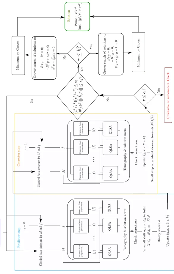
To summarize all the components in our quantum Predictor-Corrector algorithm and the interrelations among them, we show a diagram in Fig. 1 in the form of a flow chart of actions from the initializa-tion to the terminainitializa-tion of the quantum algorithm providing the solution to the given (LP) and (LD) problems in (2) and (3).
IV. CONCLUSIONS
Quantization of Linear Programming problems thus far have been achieved by using multiplica-tive weight methods as in the pioneering work of Brand˜ao and Svore for Semidefinite Programming (SDP) problems [22], which are more general than Linear Programming problems. In this work, we have enlarged the range of applicability of quantum
algorithms for Linear Programming problems by us-ing Interior Point methods instead. Specifically, our quantum algorithm relies on a type of Interior Point algorithm known as the Predictor-Corrector method that is very well behaved with respect to the feasi-bility, optimality conditions of the output solution and the iteration complexity.
The core of our quantum Interior Point algorithm is the application of block encoding techniques as a Quantum Linear System Algorithm [2] to an
auxil-...
...
FIG. 2. Scheme of the algorithm.
iary system of equations that comprises an homo-geneous self-dual primal-dual problem associated to the original Linear Programming problem. This is the basis of the Predictor-Corrector method, from which many of its good properties derive. In par-ticular, the iteration complexity of the classical part scales as the square root of the size n of the cost function. Then, the advantage of the quantum part of the Predictor-Corrector algorithm amounts to a faster solution of the linear system of equations, with complexityO((n+m)√n+m) including the readout process, as can be seen in table I.
Hence, this quantum Predictor Corrector algo-rithm is an hybrid algoalgo-rithm, partially classical, par-tially quantum. Applying the QLSA is not an easy task if we want to achieve a clear advantage. These algorithms come with several shortcomings, some of which have been recently overcome [51] for sparse linear systems. Also, even though the solution to the system of linear equations can be obtained in a quantum state, then it is not easy to extract all the information provided by the solution. One has to be
satisfied by obtaining partial information from the encoded solution such as an expectation value of in-terest or a single entry of the vector solution. Never-theless this does not stop us from obtaining a poly-nomial quantum advantage in the number of vari-ables of the problem n, if the matrix is dense, well-conditioned, with m =O(n), and with a constant-bounded spectral norm.
ACKNOWLEDGEMENTS
We acknowledge financial support from the Span-ish MINECO grants FIS2015-67411P, and the CAM research consortium QUITEMAD-CM, Grant No.S2018/TCS-4342. The research of M.A.M.-D. has been partially supported by the U.S. Army Re-search Office through Grant No. W911NF-14-1-0103. P. A. M. C. thanks the support of a FPU MECD Grant.
[1] Y. Ye, M. J. Todd, and S. Mizuno, “An o(√nl )-iteration homogeneous and self-dual linear program-ming algorithm,” Mathematics of Operations Re-search, vol. 19, no. 1, pp. 53–67, 1994.
[2] S. Chakraborty, A. Gily´en, and S. Jeffery, “The power of block-encoded matrix powers: improved regression techniques via faster hamiltonian simula-tion,”arXiv preprint arXiv:1804.01973, 2018. [3] E. D. Nering and A. W. Tucker, Linear Programs
& Related Problems: A Volume in the Computer Science and Scientific Computing Series. Elsevier, 1992.
[4] M. Padberg, Linear optimization and extensions, vol. 12. Springer Science & Business Media, 2013. [5] K. G. Murty, Linear programming, vol. 60. Wiley
New York, 1983.
[6] S. J. Russell and P. Norvig, Artificial intelligence: a modern approach. Pearson Education Limited,, 2016.
[7] M. Mohri, A. Rostamizadeh, and A. Talwalkar,
Foundations of machine learning. MIT press, 2012. [8] L. Vandenberghe and S. Boyd, “Semidefinite pro-gramming,”SIAM review, vol. 38, no. 1, pp. 49–95, 1996.
[9] M. J. Todd, “Semidefinite optimization,”Acta Nu-merica, vol. 10, pp. 515–560, 2001.
[10] M. Laurent and F. Rendl,Semidefinite programming and integer programming. Centrum voor Wiskunde en Informatica, 2002.
[11] E. De Klerk, Aspects of semidefinite programming: interior point algorithms and selected applications, vol. 65. Springer Science & Business Media, 2006. [12] J. Preskill, “Quantum computing in the nisq era and
beyond,”arXiv preprint arXiv:1801.00862, 2018. [13] D. Nigg, M. Mueller, E. A. Martinez, P. Schindler,
M. Hennrich, T. Monz, M. A. Martin-Delgado, and R. Blatt, “Quantum computations on a topologi-cally encoded qubit,”Science, p. 1253742, 2014. [14] R. Barends, J. Kelly, A. Megrant, A. Veitia,
D. Sank, E. Jeffrey, T. C. White, J. Mutus, A. G. Fowler, B. Campbell, et al., “Superconducting quantum circuits at the surface code threshold for fault tolerance,” Nature, vol. 508, no. 7497, p. 500, 2014.
[15] A. D. C´orcoles, E. Magesan, S. J. Srinivasan, A. W. Cross, M. Steffen, J. M. Gambetta, and J. M. Chow, “Demonstration of a quantum error detection code using a square lattice of four superconduct-ing qubits,”Nature communications, vol. 6, p. 6979, 2015.
[16] J. Preskill, “Quantum computing and the entan-glement frontier,” arXiv preprint arXiv:1203.5813, 2012.
[17] S. Aaronson and A. Arkhipov, “The computational complexity of linear optics,” in Proceedings of the forty-third annual ACM symposium on Theory of computing, pp. 333–342, ACM, 2011.
[18] P. W. Shor, “Polynomial-time algorithms for prime factorization and discrete logarithms on a quantum
computer,” SIAM review, vol. 41, no. 2, pp. 303– 332, 1999.
[19] L. K. Grover, “Quantum mechanics helps in search-ing for a needle in a haystack,”Physical review let-ters, vol. 79, no. 2, p. 325, 1997.
[20] M. A. Nielsen and I. Chuang,Quantum computation and quantum information. Cambridge, Cambridge University Press, 2000.
[21] A. Galindo and M. A. Martin-Delgado, “Informa-tion and computa“Informa-tion: Classical and quantum as-pects,” Reviews of Modern Physics, vol. 74, no. 2, p. 347, 2002.
[22] F. G. Brandao and K. M. Svore, “Quantum speed-ups for solving semidefinite programs,” in Founda-tions of Computer Science (FOCS), 2017 IEEE 58th Annual Symposium on, pp. 415–426, IEEE, 2017. [23] F. G. Brandao, A. Kalev, T. Li, C. Y.-Y. Lin,
K. M. Svore, and X. Wu, “Exponential quantum speed-ups for semidefinite programming with ap-plications to quantum learning,” arXiv preprint arXiv:1710.02581, 2017.
[24] J. Van Apeldoorn, A. Gily´en, S. Gribling, and R. de Wolf, “Quantum sdp-solvers: Better upper and lower bounds,” in Foundations of Computer Science (FOCS), 2017 IEEE 58th Annual Sympo-sium on, pp. 403–414, IEEE, 2017.
[25] J. van Apeldoorn and A. Gily´en, “Improvements in quantum sdp-solving with applications,” arXiv preprint arXiv:1804.05058, 2018.
[26] S. Chakrabarti, A. M. Childs, T. Li, and X. Wu, “Quantum algorithms and lower bounds for convex optimization,” arXiv preprint arXiv:1809.01731, 2018.
[27] L. G. Khachiyan, “A polynomial algorithm in linear programming,” in Doklady Academii Nauk SSSR, vol. 244, pp. 1093–1096, 1979.
[28] N. Karmarkar, “A new polynomial-time algorithm for linear programming,” inProceedings of the six-teenth annual ACM symposium on Theory of com-puting, pp. 302–311, ACM, 1984.
[29] F. A. Potra and S. J. Wright, “Interior-point meth-ods,”Journal of Computational and Applied Math-ematics, vol. 124, no. 1-2, pp. 281–302, 2000. [30] S. Mizuno, M. J. Todd, and Y. Ye, “On
adaptive-step primal-dual interior-point algorithms for lin-ear programming,” Mathematics of Operations re-search, vol. 18, no. 4, pp. 964–981, 1993.
[31] J. R. Shewchuk et al., “An introduction to the conjugate gradient method without the agonizing pain,” 1994.
[32] W. H. Press, B. P. Flannery, S. A. Teukolsky, W. T. Vetterling, et al., Numerical recipes, vol. 2. Cam-bridge university press CamCam-bridge, 1989.
[33] V. Pan and J. Reif, “Fast and efficient parallel solu-tion of dense linear systems,”Computers & Mathe-matics with Applications, vol. 17, no. 11, pp. 1481– 1491, 1989.
[34] I. Kerenidis and A. Prakash, “A quantum inte-rior point method for lps and sdps,”arXiv preprint
arXiv:1808.09266, 2018.
[35] G. Nannicini, “Fast quantum subroutines for the simplex method,”arXiv preprint arXiv:1910.10649, 2019.
[36] K. M. Anstreicher, J. Ji, F. A. Potra, and Y. Ye, “Average performance of a self–dual interior point algorithm for linear programming,” inComplexity in numerical optimization, pp. 1–15, World Scientific, 1993.
[37] A. Aspuru-Guzik, A. D. Dutoi, P. J. Love, and M. Head-Gordon, “Simulated quantum computa-tion of molecular energies,” Science, vol. 309, no. 5741, pp. 1704–1707, 2005.
[38] A. Kandala, A. Mezzacapo, K. Temme, M. Takita, M. Brink, J. M. Chow, and J. M. Gambetta, “Hardware-efficient variational quantum eigensolver for small molecules and quantum magnets,”Nature, vol. 549, no. 7671, p. 242, 2017.
[39] M.-H. Yung, J. Casanova, A. Mezzacapo, J. Mc-clean, L. Lamata, A. Aspuru-Guzik, and E. Solano, “From transistor to trapped-ion computers for quantum chemistry,” Scientific reports, vol. 4, p. 3589, 2014.
[40] C. Hempel, C. Maier, J. Romero, J. McClean, T. Monz, H. Shen, P. Jurcevic, B. Lanyon, P. Love, R. Babbush, et al., “Quantum chemistry calcula-tions on a trapped-ion quantum simulator,” arXiv preprint arXiv:1803.10238, 2018.
[41] Y. Cao, J. Romero, J. P. Olson, M. Degroote, P. D. Johnson, M. Kieferov´a, I. D. Kivlichan, T. Menke, B. Peropadre, N. P. Sawaya,et al., “Quantum chem-istry in the age of quantum computing,” arXiv preprint arXiv:1812.09976, 2018.
[42] A. W. Harrow, A. Hassidim, and S. Lloyd, “Quan-tum algorithm for linear systems of equations,”
Physical review letters, vol. 103, no. 15, p. 150502, 2009.
[43] L. Wossnig, Z. Zhao, and A. Prakash, “Quantum linear system algorithm for dense matrices,” Physi-cal review letters, vol. 120, no. 5, p. 050502, 2018. [44] D. Coppersmith and S. Winograd, “Matrix
multipli-cation via arithmetic progressions,”Journal of sym-bolic computation, vol. 9, no. 3, pp. 251–280, 1990. [45] S. Arora and S. Kale, “A combinatorial, primal-dual
approach to semidefinite programs,” in Proceedings of the thirty-ninth annual ACM symposium on The-ory of computing, pp. 227–236, ACM, 2007. [46] I. Kerenidis and A. Prakash, “Quantum
recommen-dation systems,” in Proceedings of the 8th Innova-tions in Theoretical Computer Science Conference, 2017.
[47] A. Montanaro and S. Pallister, “Quantum algo-rithms and the finite element method,”Physical Re-view A, vol. 93, no. 3, p. 032324, 2016.
[48] G. H. Low and I. L. Chuang, “Hamiltonian simula-tion by qubitizasimula-tion,”Quantum, vol. 3, p. 163, 2019. [49] C. Wang and L. Wossnig, “A quantum algorithm for simulating non-sparse hamiltonians,”arXiv preprint arXiv:1803.08273, 2018.
[50] A. M. Childs, R. Kothari, and R. D. Somma, “Quantum algorithm for systems of linear equations
with exponentially improved dependence on preci-sion,”SIAM Journal on Computing, vol. 46, no. 6, pp. 1920–1950, 2017.
[51] B. D. Clader, B. C. Jacobs, and C. R. Sprouse, “Preconditioned quantum linear system algorithm,”
Physical review letters, vol. 110, no. 25, p. 250504, 2013.
[52] V. V. Shende, S. S. Bullock, and I. L. Markov, “Syn-thesis of quantum-logic circuits,” IEEE Transac-tions on Computer-Aided Design of Integrated Cir-cuits and Systems, vol. 25, no. 6, pp. 1000–1010, 2006.
[53] L. Grover and T. Rudolph, “Creating superpositions that correspond to efficiently integrable probability distributions,” arXiv preprint quant-ph/0208112, 2002.
[54] Y. R. Sanders, G. H. Low, A. Scherer, and D. W. Berry, “Black-box quantum state preparation with-out arithmetic,” Physical review letters, vol. 122, no. 2, p. 020502, 2019.
[55] A. Gily´en, Y. Su, G. H. Low, and N. Wiebe, “Quan-tum singular value transformation and beyond: ex-ponential improvements for quantum matrix arith-metics,”arXiv preprint arXiv:1806.01838, 2018. [56] A. Ambainis, “Variable time amplitude
amplifi-cation and quantum algorithms for linear alge-bra problems,” in STACS’12 (29th Symposium on Theoretical Aspects of Computer Science), vol. 14, pp. 636–647, LIPIcs, 2012.
[57] Y. Ye, “On the finite convergence of interior-point algorithms for linear programming,” Mathematical Programming, vol. 57, no. 1-3, pp. 325–335, 1992. [58] L. A. B. Kowada, C. Lavor, R. Portugal, and C. M.
De Figueiredo, “A new quantum algorithm for solv-ing the minimum searchsolv-ing problem,”International Journal of Quantum Information, vol. 6, no. 03, pp. 427–436, 2008.
[59] E. Tang, “A quantum-inspired classical algo-rithm for recommendation systems,”arXiv preprint arXiv:1807.04271, 2018.
[60] N.-H. Chia, H.-H. Lin, and C. Wang, “Quantum-inspired sublinear classical algorithms for solv-ing low-rank linear systems,” arXiv preprint arXiv:1811.04852, 2018.
[61] J. M. Arrazola, A. Delgado, B. R. Bardhan, and S. Lloyd, “Quantum-inspired algorithms in prac-tice,”arXiv preprint arXiv:1905.10415, 2019. [62] D. Nagaj, P. Wocjan, and Y. Zhang, “Fast
ampli-fication of qma,” arXiv preprint arXiv:0904.1549, 2009.
Appendix A: Calculation of the error0 in the Corrector step
In this appendix we want to calculate the size of the error0 we need in order to make the Corrector step successfully output a point withinN(1/4), and its comparison with the complexity of the quantum subroutine.
To prove this suppose we definexas the concate-nation ofxt andτt, andsas concatenating stand kt. Callx0ands0 the exact arithmetic solution, so that being0 the error of the quantum subroutine
x=x0+0x1; s=s0+s1; ||s1||=||x1|| ≤n+1. (A1) since each entry will have an error of0 at most, and then each entry in x1 and s1 are, say, at most 1. Using (14), we can see that
X0s0−1 xT 0s0 n+ 1 ≤ 1 4√2 xT 0s0 n+ 1, (A2)
and we want to calculate how small 0 needs to be in order to comply with
Xs−1x Ts n+ 1 ≤1 4 xTs n+ 1. (A3)
Expanding, to leading orderO(0)
Xs−1x Ts n+ 1 = (A4) ||X0s0+0(X0s1+X1s0) (A5) −1x T 0s0+0(x T 0s1+x T 1s0) n+ 1 (A6) ≤ X0s0−1x T 0s0 n+ 1 (A7) +0 X0s1−1x T 0s1 n+ 1 (A8) +0 X1s0−1 xT 1s0 n+ 1 . (A9)
The first term is clearly our hypothesis (A2), so let us calculate one of other two terms (calculating one is the same as calculating the other, they are sym-metrical). Letxi = (¯xi,1, ...,x¯i,n+1)T fori ∈ {0,1} and similarly for si, and let us expand the
expres-sion. X1s0−1x T 1s0 n+ 1 = (A10) v u u u t n+1 X i=1 x¯1,is¯0,i− 1 n+ 1 n+1 X j=1 ¯ x1,js¯0,j 2 = (A11) n+1 X i=1 x¯ 2 1,i¯s 2 0,i− 2 n+ 1x¯1,i¯s0,i n+1 X j=1 ¯ x1,js¯0,j (A12) + 1 (n+ 1)2 n+1 X j=1 ¯ x1,j¯s0,j 2 1/2 = (A13) n+1 X i=1 ¯ x21,i¯s20,i− 2 n+ 1 n+1 X i,j=1 ¯ x1,is¯0,ix¯1,js¯0,j (A14) + n+ 1 (n+ 1)2 n+1 X i,j=1 ¯ x1,is¯0,ix¯1,js¯0,j 1/2 (A15)
Now we can see that the second term partially can-cels out with the third
n+1 X i=1 ¯ x21,i¯s20,i− 1 n+ 1 n+1 X i,j=1 ¯ x1,is¯0,i¯x1,j¯s0,j 1/2 (A16) = ||X1s0||2− 1 n+ 1(x T 1s0) 2 1/2 (A17)
Therefore, we can write
Xs−1 x Ts n+ 1 ≤ 1 4√2 xT 0s0 n+ 1 (A18) +0 ||X1s0||2− 1 n+ 1(x T 1s0) 2 1/2 (A19) + ||X0s1||2− 1 n+ 1(x T 0s1)2 1/2! (A20)
Enforcing (A3) can be done if we choose0 such that 1 4√2 xT 0s0 n+ 1 + 0 ||X1s0||2− 1 n+ 1(x T 1s0)2 1/2 (A21) + ||X0s1||2− 1 n+ 1(x T 0s1) 2 1/2! (A22) ≤ 1 4 xTs n+ 1 = 1 4 (x0+0x1)T(s0+0s1) n+ 1 . (A23)
To leading orderO(0) that means 1 4√2 xT0s0 n+ 1+ 0 ||X1s0||2− 1 n+ 1(x T 1s0) 2 1/2 (A24) + ||X0s1||2− 1 n+ 1(x T 0s1)2 1/2! ≤ (A25) 1 4 xT0s0 n+ 1+ 0 4 xT1s0+xT0s1 n+ 1 , (A26) or equivalently 2−√2 8 xT 0s0 n+ 1 ≥ (A27) 0 ||X1s0||2− 1 n+ 1(x T 1s0)2 1/2 (A28) + ||X0s1||2− 1 n+ 1(x T 0s1) 2 1/2 −1 4 xT 1s0+xT0s1 n+ 1 ! , (A29) implying 0≤ 2−√2 8 xT 0s0 n+1 h ||X1s0||2− 1 n+1(x T 1s0)2 i1/2 +h||X0s1||2− 1 n+1(x T 0s1)2 i1/2 −1 4 xT 1s0+xT0s1 n+1 . (A30)
Let us start analyzing the denominator. The worst case is that the denominator is very large so it forces the error to be small. The fraction 1
4
xT1s0+xT0s1 n+1 could turn negative, thus increasing the denomi-nator. But we can see that its influence will be low due to its denominator n+ 1. Due to (A1), we can expect xT 1s0 ≤ (n+ 1) maxi|s¯0,i| = O(n) and xT 0s1 ≤ (n+ 1) maxi|x¯0,i| =O(n). Therefore 1 4 xT1s0+xT0s1 n+1 =O(1).
Additionally, if all entries in x0 ands0 are O(1) it is easy to check that ||X0s1||2 = O(n) and
||X1s0||2 = O(n). Therefore the denominator will beO(n1/2).
The numerator of (A30) is a bit more tricky. In this case the worst case is when it is small. What seems the biggest problem is that [1] tells us that in the exact solution xT0s0 = 0, and furthermore it is divided byn+1. Therefore we can see that in the ex-act solutionshould be 0 (which is what we should expect). What matters is the convergence speed. At the beginning recall that x0 = s0 = [1, ...,1]T. Therefore, at the very beginning xT0s0
n+1 = 1. Accord-ing to [1], every two iterationsxT
0s0should decrease at a rate (1−1/(√4
8√n+ 1)). The question there-fore is what happens afterO(L√nt¯) iterations (the iterations of the algorithm).
This finally gives us the threshold for0 we would like in order to stay insideN(1/4):
0≤ lim n→∞O(n −1/2) 1−√4 1 8√n O(L √ n¯t) =O(n−1/2)e−O(L¯t). (A31)
Since L = logn in the usual case and ¯t = max[log((x0)T(s0)/(123)),log(||(¯b
T,c¯T)||/ 23)], the error threshold is 0=O(n−poly logn−1/2).
On the other hand, the complexity on the pre-cision of the algorithm is O(−2) and the differ-ence in complexity in n that we stated in tabla I between our algorithm and the ‘best classical’ al-gorithm is O(√n). This means that in order to maintain the quantum advantage one would want ≤O(n−1/4). Therefore we have seen that setting an 0 small enough might be too expensive compu-tationally in general for the quantum subroutine.
Appendix B: Gradient descent for shifting the output of the corrector step.
We have seen that setting an 0 small enough might be too expensive computationally. Therefore let us try something: choose a small precision on the error for the corrector step0=O(n−1/a), and then, once we get the result, perform one step gradient descent of the size00 towardsN(1/4).
For that call, using the definition ofN(β) (14),
g(x, s) = Xs−1x Ts n+ 1 2 −β2 xTs n+ 1 2 . (B1)
Using the equivalent to (A16), we can rewrite it like g(x, s) =||Xs−1µ||2−β2µ2 (B2) = X i ¯ x2is¯2i − 1 n+ 1 n+1 X i,j=1 ¯ xisi¯xj¯ sj¯ (B3) − β 2 (n+ 1)2 n+1 X i,j=1 ¯ xi¯si¯xjsj¯ (B4) =X i ¯ x2i¯s2i − β2+ (n+ 1) (n+ 1)2 n+1 X i,j=1 ¯ xisi¯xj¯ ¯sj. (B5)
Notice that the points that are inN(β) are those for whichg(x, s)≤0. We calculate the gradient, calling B= β2(+(n+1)n+1)2 =O(n−1): dg(x, s) dx¯k = 2¯xk¯s2k−2B X i ¯ xi¯si¯sk. (B6) Clearly, dg(x, s) d¯sk = 2¯skx¯ 2 k−2B X i ¯ sixi¯xk.¯ (B7)
The idea is now, supposing that
X0s0−1x T 0s0 n+ 1 2 ≤β2 xT 0s0 n+ 1 2 , (B8)
if we can find00=O(n−1/a) such that
Xs−00 Xdg ds +S dg dx (B9) −1 1 n+ 1 xTs−00 xTdg ds+s Tdg dx 2 (B10) ≤ β 2 (n+ 1)2 xTs−00 xTdg ds +s Tdg dx 2 . (B11) For that, as it will be very useful, first calculate to leading orderO(00) X i ¯ xi−00dg dxi¯ si¯ − 00dg d¯si = X i xi¯ ¯si−200(¯s2i + ¯x2i) ¯sixi¯ −B X j ¯ xj¯sj . (B12) We can write, to leading order O(), how much is
||Xs||2in the new point:
X i ¯ si−00dg d¯si 2 ¯ xi−00 dg dxi¯ 2 = X i x¯ 2 is¯ 2 i −400x¯i¯si(¯s2i + ¯x 2 i) s¯ix¯i−B X j ¯ xj¯sj . (B13)
The next thing we want to calculate is, to leading order O(), the new value of (xTs)2
X i,j ¯ si−00dg d¯si xi¯ − 00dg dxi¯ ¯ sj−00dg d¯sj xj¯ − 00 dg dxj¯ =X i,j ¯ xixj¯ si¯sj¯ −X i,j 400xj¯ sj¯(¯s2i + ¯x2i) si¯xi¯ −BX k ¯ xk¯sk ! (B14)
We now have all the parts we need to calculate the result we were seeking. Let us try to check that we can make g x−00dg dx,s− 00dg ds ≤0. (B15) Let’s check it g x−00dg dx,s− 00dg ds = =X i ¯ x2i¯s2i −B n+1 X i,j=1 ¯ xi¯sixj¯ ¯sj+ −400 X i ¯ xisi¯(¯s2i + ¯x2i) si¯xi¯ −B X j ¯ xj¯sj −BX i,j ¯ xjsj¯(¯s2i + ¯x2i) si¯xi¯ −B X k ¯ xk¯sk ! (B16)
This allows us to calculate the approximate 00 in time O(n) such that the point is inN(1/4). Is this 00 large? To answer that question expand in x =
x0+0x1 ands=s0+0s1 g x−00dg dx,s− 00dg ds = =X i ¯ x2i,0s¯2i,0−B n+1 X i,j=1 ¯ xi,0s¯i,0x¯j,0¯sj,0+ + 20 " X i (¯xi,0xi,¯ 1¯s2i,0+ X i ¯ x2i,0¯si,0si,¯ 1) −BX i,j (¯xi,1s¯i,0¯xj,0s¯j,0+ ¯xi,0¯si,1x¯j,0¯sj,0) −400 X i ¯ xi¯si(¯s2i + ¯x 2 i) s¯ix¯i−B X j ¯ xjs¯j −BX i,j ¯ xj¯sj(¯s2i + ¯x2i) si¯xi¯ −BX k ¯ xksk¯ ! . (B17)
We know by hypothesis that the second line of (B17) is less than 0 (the exact point is inN(1/4)). There-fore we want the term of 00 to cancel that of 0. Notice that this means that 00 =O(0), since both terms in the square brackets are of sizeO(n). There-fore, we are only introducing an error of size O(0), which is what we already had, but we can now en-sure that the output is in N(1/4). (B16) explains how to calculate00 such that, to orderO(00) we are insideN(1/4); and (B17) certifies that00=O(0).
Since in the expansion we have only consider terms up to00, there is the possibility that after this shift we are still outside N(1/4). However, in this case, we will only be002=O(02) away fromN(1/4), so it-erating this process we can make this errorO(002i), which decreases quickly on the iteration i. Alter-natively one could take into account further terms with higher exponents of00in the expansions (B12), (B13) and (B14).
Further, one could also wonder if the gradient step could converge towards different local minima of g(x, s) than those in the central path. However, it is easy to check using (B6) and (B7) that all lo-cal minima (or maxima or saddle points) fulfil either xi= 0 andsi= 0, or
xisi−B
X
j
xjsj = 0 (B18)
for alli∈ {1, ..., n+ 1}. Substituting those points in
the definition of g(x, s) (B5), g= n+1 X i=1 x2is2i − β2+ (n+ 1) (n+ 1)2 (n+ 1) n+1 X i=1 x2is2i = 1− β 2 n+ 1 −1 n+1 X i=1 x2is2i ≤0. (B19) This means that all those points are within N(β), so the gradient step will be taken towards N(β).
With this we conclude that with an O(0)-shift to the output of the alreadyO(0)-precise Corrector step we can ensure that the point is in N(1/4).
Appendix C: Convergence of the algorithm
The legitimacy of the previous procedure rests on the fact that we only have to check that we do not get out of the neighbourhood of the central path. However, a question remains: does the algorithm still converges, with this modification, in O(n1/2L) steps? In this appendix we analyse this question and find a positive answer. The references we will be using are [30], mainly, and [1].
Let us first review how the convergence is studied in the original article [1]. The convergence happens when the duality gap µcloses. In those references, one proves that in the corrector step µk = µk+1. The convergence happens in the predictor corrector, where the duality gap µk+1 = (1−α)µk. Lets see these two things.
For convenience definextconcatenatingxtandτt; st as the concatenation of st and κt; and similarly with dx, dτ, andds anddκ. The starting equation is µt+1(δ) =(x t+1)Tst+1 n+ 1 = (xt)Tst+δ((xt)Tds+ (st)Tdx) +δ2dTxds n+ 1 . (C1) Since the exact solution fulfils equation (15b), that would mean that
Xtds+Stdx=γtµt1−Xtst. (C2) In practice, since we get an approximation solution, we can substitute the term multiplied by δ in (C1) withγtµt(n+1)−(xt)Tst+(xt)Tx+(st)Ts, where xand s are the error vectors in the estimation of dxandds respectively.
On the other hand, using equation (15a) for the exact solution, and the second part of theorem 5 of