Developing a procedure to identify parameters for calibration of a vissim model

(1)

DEVELOPING A PROCEDURE TO IDENTIFY PARAMETERS FOR

CALIBRATION OF A VISSIM MODEL

A Thesis Presented to The Academic Faculty

by

David Michael Miller

In Partial Fulfillment

of the Requirements for the Degree Masters of Science in the

School of Civil & Environmental Engineering

Georgia Institute of Technology May 2009

(2)

DEVELOPING A PROCEDURE TO IDENTIFY PARAMETERS FOR

CALIBRATION OF A VISSIM MODEL

Approved by:

Dr. Michael Hunter, Advisor

Georgia Institute of Technology

Dr. Michael Rodgers

Dr. Jorge Laval

(3)

iii

ACKNOWLEDGMENTS

First, I would like to thank Dr. Michael Hunter and Dr. Michael Rodgers for their invaluable input into the development and completion of this thesis. I would also like to thank Patrick Robert Burns for providing assistance in computer programming that made the project possible. Additionally, I would like to thank Captain Wayne Radloff for his support of my research and graduate studies. Finally, I would like to thank my parents, Bruce and Tamara Miller, and my fiancée, Grace McGee, for their continuing support and guidance.

(4)

iv TABLE OF CONTENTS ACKNOWLEDGMENTS iii LIST OF TABLES ix LIST OF FIGURES x SUMMARY xvi CHAPTER 1: INTRODUCTION 1 1.1 Study Need 1 1.2 Study Objective 2 1.3 Study Overview 2 1.3.1 Background 2 1.3.2 Literature Review 2 1.3.3 General Procedure 3

1.3.4 Case Study: Cobb Parkway Model 3

CHAPTER 2: BACKGROUND 4

2.1 VISSIM Overview 4

2.2 Network Representation 5

2.3 Driving Behavior 7

2.3.1 Following Behavior 7

(5)

v

2.3.3 Lateral Behavior 10

2.3.4 Signal Control Behavior 10

2.4 Model Calibration 11

2.5 Output Files 15

2.5.1 Travel Time 15

2.5.2 Delay 16

2.5.3 Queue Length 16

2.5.4 Distribution of Green Times 18

2.5.5 Error Files 18

2.6 Input Files 20

CHAPTER 3: LITERATURE REVIEW 21

3.1 Previous Related Studies 21

3.1.1 Calibration of VISSIM for Shanghai Expressway

Using Genetic Algorithm (2005) 21

3.1.2 VISSIM: A Multi-Parameter Sensitivity Analysis (2006) 23 3.1.3 Microscopic Simulation Model Calibration and Validation, Case Study of VISSIM Simulation Model for a Coordinated Actuated

Signal System (2003) 25

3.1.4 Development and Evaluation of a Procedure for the Calibration of

Simulation Models (2005) 27

3.1.5 Application of Microscopic Simulation Model Calibration and Validation Procedure: A Case Study of Coordinated Actuated

(6)

vi

3.1.6 A Methodology to Calibrate Microsimulation Models for Traffic at Signalized Intersections with a High Degree of Heterogeneity and

Lack of Lane Discipline (2008) 30

3.1.7 Development and Evaluation of a Calibration and Validation Procedure for Microscopic Simulation Models (2004) 32

3.2 Analysis 33

CHAPTER 4: GENERAL PROCEDURE 35

4.1 Initial Parameter Selection 35

4.2 Measures of Effectiveness Selection 36

4.3 Monte Carlo Experiment 37

4.3.1 Parameter Range Selection 37

4.3.2 Random Parameter Generation 38

4.3.3 Simulation Runs 39

4.4 Sensitivity Analysis and Parameter Elimination 40

4.4.1 Plotting the Results 40

4.4.2 Analyzing the Results 41

4.4.3 Parameter Elimination 42

4.4.4 Iteration 43

CHAPTER 5: CASE STUDY: COBB PARKWAY MODEL 45

5.1. Introduction 45

5.1.1 Model Selection 45

(7)

vii

5.2.1 Model Location and Characteristics 46

5.2.2 Calibration with a Genetic Algorithm 49

5.3 Initial Parameter Selection 49

5.3.1 Base Distributions 50

5.3.2 Following Behavior Parameters 50

5.3.3 Lane Change Behavior Parameters 51

5.3.4 Lateral Behavior Parameters 51

5.3.5 Signal Control Behavior Parameters 52

5.3.6 Connector Parameters 52

5.4 Measures of Effectiveness Selection 52

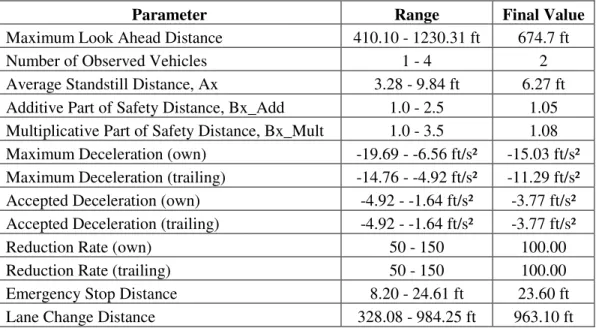
5.5. Parameter Range Selection 56

5.6 1st Parameter Set Results 60

5.6.1 100% Volume Results 60

5.7 2nd Parameter Set Results 70

5.7.1 Comparison to the 1st Parameter Set Results 70

5.7.3 75% Volume Results 77

5.8 3rd Parameter Set Results 78

(8)

viii

5.9 Conclusions 81

APPENDIX A: 100% VOLUME SCENARIO RESULTS 84

APPENDIX B: 75% VOLUME SCENARIO RESULTS 127

(9)

ix

LIST OF TABLES

Table 1: Complete List of Parameters [13] 12

Table 2: Common VISSIM Simulation Errors [13] 18

Table 3: Existing Calibration Data for the Cobb Parkway Model 49 Table 4: Comparison of Average Travel Times

with and without Lateral Behavior Parameters 52

Table 5: Example Data Used to Define Ranges 56

Table 6: Initially Selected Parameter Ranges 59

Table 7: 1st Round 100% Volume Scenario, Parameter's

Effect on the Mean of the Travel Times for Retained Parameters 61 Table 8: 1st Round 100% Volume Scenario, Parameter's

Effect on the Mean of the Travel Times for Eliminated Parameters 61 Table 9: 1st Round 75% Volume Scenario, Parameter's

Effect on the Mean of the Travel Times for Retained Parameters 69 Table 10: 1st Round 75% Volume Scenario, Parameter's

Effect on the Mean of the Travel Times for Eliminated Parameters 69 Table 11: 2nd Round 100% Volume Scenario, Parameter's

Effect on the Mean of the Travel Times for Retained Parameters 76 Table 12: 2nd Round 100% Volume Scenario, Parameter's

Effect on the Mean of the Travel Times for Eliminated Parameters 76 Table 13: 2nd Round 75% Volume Scenario, Parameter's

Effect on the Mean of the Travel Times for Retained Parameters 77 Table 14: 2nd Round 100% Volume Scenario, Parameter's

Effect on the Mean of the Travel Times for Eliminated Parameters 77 Table 15: Final 100% Volume Scenario, Parameter's

Effect on the Mean of the Travel Times for Retained Parameters 80 Table 16: Final 75% Volume Scenario, Parameter's

(10)

x

LIST OF FIGURES

Figure 1: VISSIM Modules [13] 4

Figure 2: Necessary Lane Change Parameters [13] 9

Figure 3: Illustration of a Latin Hypercube Sample [3] 26

Figure 4: Satellite Image of Cobb Parkway [1] 47

Figure 5: Map of Model Location [1] 47

Figure 6: Network Representation in VISSIM 48

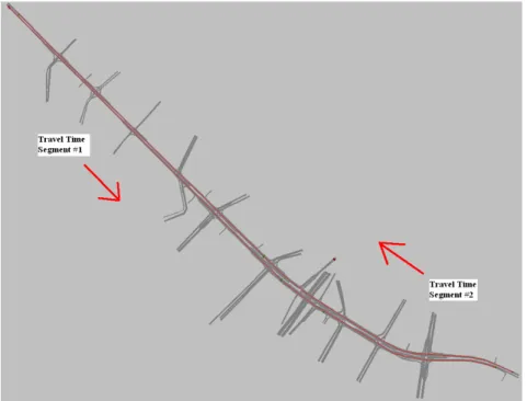
Figure 7: Travel Time Segments #1 and #2 53

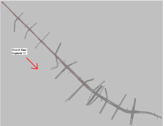
Figure 8: Travel Time Segment #3 54

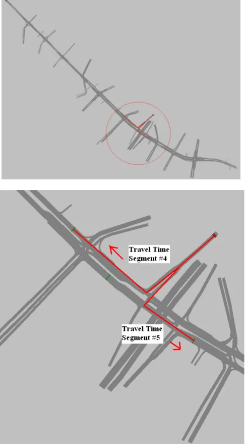
Figure 9: Detail View of Travel Time Segments #4 and #5 55 Figure 10: Average Travel Times on Segment #5 vs. the Average Standstill distance 57 Figure 11: Average Travel Times on Segment #3 vs. the Minimum Headway 62 Figure 12: Average Standstill Distance Effect on the

Mean Travel Time for each Segment 63

Figure 13: Maximum Deceleration (trailing) Effect on the

Figure 14: Average Travel Times on Segment #2

vs. Reduction Factor for Changing Lanes before a Signal 65 Figure 15: Average Travel Times on Segment #1

vs. the Look Ahead Distance Minimum 66

Figure 16: Accepted Deceleration (own) Effect on the

Figure 17: Additive Part of Safety Distance Effect on the

Figure 18: 100% Volume Comparison of Average Travel Times from the

(11)

xi

1st and 2nd Parameter Set Runs 71

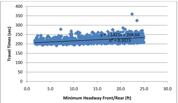
Figure 20: Queue Downstream of Travel Time Segment #5 Blocking Traffic 72 Figure 21: Relationship between the Minimum Headway and Travel Times on

Travel Time Route #1 and the Minimum Headway and Travel Times on

Travel Time Route #5 for 100% Volume Scenario of Iteration #2. 73 Figure 22: Average Travel Times on Segment #3

vs. the Desired Speed Distribution Range (30 mph trial) 75 Figure 23: Desired Speed Distribution Range Effect on the

Mean Travel time for each Segment (30 mph trial) 75

1st, 2nd and 3rd Parameter Set Runs 79

Figure 26(a-e): 100% Volume Scenario, Iteration #1, Parameter #1 Scatter Plots 85

(12)

xii

(13)

xiii

Figure 57(a-e): 100% Volume Scenario, Iteration #2, Parameter #18 Scatter Plots Figure 58(a-e): 100% Volume Scenario, Iteration #2, Parameter #22 Scatter Plots Figure 59(a-e): 100% Volume Scenario, Iteration #3, Parameter #5 Scatter Plots Figure 60(a-e): 100% Volume Scenario, Iteration #3, Parameter #6 Scatter Plots Figure 61(a-e): 100% Volume Scenario, Iteration #3, Parameter #7 Scatter Plots Figure 62(a-e): 100% Volume Scenario, Iteration #3, Parameter #8 Scatter Plots Figure 63(a-e): 100% Volume Scenario, Iteration #3, Parameter #9 Scatter Plots Figure 64(a-e): 100% Volume Scenario, Iteration #3, Parameter #15 Scatter Plots Figure 65(a-e): 100% Volume Scenario, Iteration #3, Parameter #16 Scatter Plots Figure 66(a-e): 100% Volume Scenario, Iteration #3, Parameter #17 Scatter Plots Figure 67(a-e): 100% Volume Scenario, Iteration #3, Parameter #22 Scatter Plots Figure 68(a-e): 75% Volume Scenario, Iteration #1, Parameter #1 Scatter Plots Figure 69(a-e): 75% Volume Scenario, Iteration #1, Parameter #2 Scatter Plots Figure 70(a-e): 75% Volume Scenario, Iteration #1, Parameter #3 Scatter Plots Figure 71(a-e): 75% Volume Scenario, Iteration #1, Parameter #4 Scatter Plots Figure 72(a-e): 75% Volume Scenario, Iteration #1, Parameter #5 Scatter Plots Figure 73(a-e): 75% Volume Scenario, Iteration #1, Parameter #6 Scatter Plots Figure 74(a-e): 75% Volume Scenario, Iteration #1, Parameter #7 Scatter Plots Figure 75(a-e): 75% Volume Scenario, Iteration #1, Parameter #8 Scatter Plots Figure 76(a-e): 75% Volume Scenario, Iteration #1, Parameter #9 Scatter Plots 116 117 118 119 120 121 122 123 124 125 126 129 129 130 131 132 133 134 135 136

(14)

xiv

Figure 77(a-e): 75% Volume Scenario, Iteration #1, Parameter #10 Scatter Plots 137 Figure 78(a-e): 75% Volume Scenario, Iteration #1, Parameter #11 Scatter Plots 138 Figure 79(a-e): 75% Volume Scenario, Iteration #1, Parameter #12 Scatter Plots 139 Figure 80(a-e): 75% Volume Scenario, Iteration #1, Parameter #13 Scatter Plots 140 Figure 81(a-e): 75% Volume Scenario, Iteration #1, Parameter #14 Scatter Plots 141 Figure 82(a-e): 75% Volume Scenario, Iteration #1, Parameter #15 Scatter Plots 142 Figure 83(a-e): 75% Volume Scenario, Iteration #1, Parameter #16 Scatter Plots 143 Figure 84(a-e): 75% Volume Scenario, Iteration #1, Parameter #17 Scatter Plots 144 Figure 85(a-e): 75% Volume Scenario, Iteration #1, Parameter #18 Scatter Plots 145 Figure 86(a-e): 75% Volume Scenario, Iteration #1, Parameter #19 Scatter Plots 146 Figure 87(a-e): 75% Volume Scenario, Iteration #1, Parameter #20 Scatter Plots 147 Figure 88(a-e): 75% Volume Scenario, Iteration #1, Parameter #21 Scatter Plots 148 Figure 89(a-e): 75% Volume Scenario, Iteration #1, Parameter #22 Scatter Plots 149 Figure 90(a-e): 75% Volume Scenario, Iteration #2, Parameter #1 Scatter Plots 150 Figure 91(a-e): 75% Volume Scenario, Iteration #2, Parameter #5 Scatter Plots 151 Figure 92(a-e): 75% Volume Scenario, Iteration #2, Parameter #6 Scatter Plots 152 Figure 93(a-e): 75% Volume Scenario, Iteration #2, Parameter #7 Scatter Plots 153 Figure 94(a-e): 75% Volume Scenario, Iteration #2, Parameter #8 Scatter Plots 154 Figure 95(a-e): 75% Volume Scenario, Iteration #2, Parameter #15 Scatter Plots 155 Figure 96(a-e): 75% Volume Scenario, Iteration #2, Parameter #16 Scatter Plots 156

(15)

xv

Figure 97(a-e): 75% Volume Scenario, Iteration #2, Parameter #17 Scatter Plots 157 Figure 98(a-e): 75% Volume Scenario, Iteration #2, Parameter #18 Scatter Plots 158 Figure 99(a-e): 75% Volume Scenario, Iteration #2, Parameter #22 Scatter Plots 159 Figure 100(a-e): 75% Volume Scenario, Iteration #3, Parameter #5 Scatter Plots 160 Figure 101(a-e): 75% Volume Scenario, Iteration #3, Parameter #6 Scatter Plots 161 Figure 102(a-e): 75% Volume Scenario, Iteration #3, Parameter #7 Scatter Plots 162 Figure 103(a-e): 75% Volume Scenario, Iteration #3, Parameter #8 Scatter Plots 163 Figure 104(a-e): 75% Volume Scenario, Iteration #3, Parameter #15 Scatter Plots 164 Figure 105(a-e): 75% Volume Scenario, Iteration #3, Parameter #16 Scatter Plots 165 Figure 106(a-e): 75% Volume Scenario, Iteration #3, Parameter #17 Scatter Plots 166 Figure 107(a-e): 75% Volume Scenario, Iteration #3, Parameter #22 Scatter Plots 167

(16)

xvi SUMMARY

The calibration of microscopic traffic simulation models is an area of intense study; however, additional research is needed into how to select which parameters to calibrate. In this project a procedure was designed to eliminate the parameters unnecessary for calibration and select those which should be examined for a VISSIM model.

The proposed iterative procedure consists of four phases: initial parameter selection, measures of effectiveness selection, Monte Carlo experiment, and sensitivity analysis and parameter elimination. The goal of the procedure is to experimentally determine which parameters have an effect on the selected measures of effectiveness and which do not. This is accomplished through the use of randomly generated parameter sets and subsequent analysis of the generated results.

The second phase of the project involves a case study on implementing the proposed procedure on an existing VISSIM model of Cobb Parkway in Atlanta, Georgia. Each phase of the procedure is described in detail and justifications for each parameter selection or elimination are explained. For the case study the model is considered under both full traffic volumes and a reduced volume set representative of uncongested conditions. The case study shows that the procedure is effective and that many parameters can be eliminated from

(17)

1 CHAPTER 1 INTRODUCTION

In the last few decades traffic simulation has grown into a major resource for transportation engineers. The ability to simulate a proposed project prior to implementation and evaluate the potential benefits and costs allows for significant optimization of potential projects and improvements. This of course assumes that the simulation accurately, or at least reasonably, reflects reality.

In order for a traffic simulation to accurately describe reality it must utilize a valid model and be properly calibrated. A valid model implies that the underlying simulation logic reasonably reflects real-world operations. A calibrated simulation means that the input parameters provided by the user (e.g. driver aggressiveness or desired speed) allow the simulation program’s valid model to recreate the specific network under consideration. Model calibration is a frequent area of study by transportation engineers and there are a number of proposed procedures for calibrating different simulations, such as linear regression or genetic algorithms. These methods are used in order to determine input parameters values that produce simulation results representative of field data.

1.1 Study Need

One area of model calibration in which meaningful contributions are still needed is the selection of parameters for calibration. Most calibration procedures assume only a small set of the available simulation parameters are to be included in the calibration process. However, there is usually no formal procedure for selecting these parameters other than selecting the parameters which appear to the user as most likely to have a significant effect on the simulation. An

(18)

2

incomplete set of selected parameters for calibration may lead to issues rendering the simulation imprecise or the calibration method producing unrealistic parameters values.

1.2 Study Objective

The purpose of this project is to create and test a procedure to determine which parameters should be considered for calibration in a typical transportation simulation package. The developed procedure is demonstrated on an arterial simulation utilizing the simulation program PTV VISSIM. It is anticipated that this procedure could be followed to select calibration parameter sets for other facility types (e.g. freeways, toll plaza) and simulation platforms. Final calibration of the model is not an objective of this study.

1.3 Study Overview

This study focuses on two main objectives: proposing a procedure for determining parameters for calibration and a case study to demonstrate how the procedure works in practice. A summary of each section of the report is included below.

1.3.1 Background

The second chapter discusses the inner workings of VISSIM, the simulation program used for this study. Included in the chapter are sections on the physical representation of networks with links and connectors, how driving behavior is modeled with respect to car following and lane changing, model calibration, output files and the formats available, and how input files or ".inp files" are created and read by the program.

1.3.2 Literature Review

The literature review chapter is divided into two sections. The first section is an overview of relevant previous studies. These studies are primarily related to simulation calibration for

(19)

3

freeway and urban signalized arterial models. Many of the cited studies utilize the genetic algorithm for calibration. The second section delves into the need for a procedure to determine which parameters should be included in a model's calibration.

1.3.3 General Procedure

The procedure proposed in this study is outlined and explained in this chapter. There is a section in the chapter for each of the four steps of the procedure:

1. Initial Parameter Selection

2. Measures of Effectiveness Selection 3. Monte Carlo Experiment

4. Sensitivity Analysis and Parameter Elimination

There is also a final section explaining the iterative aspect of the procedure and stopping criteria. 1.3.4 Case Study: Cobb Parkway Model

The case study presented in this chapter illustrates the proposed procedure on a 13 intersection model of Cobb Parkway in Atlanta, GA. Two scenarios are considered, one utilizing 100% of the existing AM traffic and a second with AM traffic reduced uniformly by 25% to create an uncongested scenario. The two scenarios provided similar results and show that there are between 5-10 important parameters that should be included in calibration. The parameter sets chosen are almost identical between the two scenarios.

(20)

4 CHAPTER 2 BACKGROUND

2.1 VISSIM Overview

“VISSIM is a discrete, stochastic, time step based microscopic traffic flow simulation model” [13]. VISSIM 4.30 was used for this study. The model uses two different modules to produce the output: a traffic simulator and a signal state generator. The signal state generator determines the signal status at each time step and returns the value to the traffic simulator as shown in Figure 1. The traffic simulator in VISSIM allows drivers to react to vehicles ahead of them as well as vehicles to either side of the driver. Drivers are also given a higher measure of alertness as they get nearer to a traffic signal [13].

Figure 1: VISSIM Modules [13]

Detector Values

Signal State

Generator

Signal Status

(21)

5

The traffic flow model used by the traffic simulator relies on one of the following models: the “Wiedemann 74” car following model or the “Wiedemann 99” car following model. The Wiedemann 74 car following model is a psycho-physical driver behavior model developed by Wiedemann at the Technical University of Karlsruhe, Germany in 1974 [16]. The basic premise of the model is that a driver will continue at a constant speed until he perceives a vehicle in front of him to be traveling either faster or slower than his current speed. Then the driver will accelerate or decelerate accordingly. Due to the driver’s imperfect perception he will overcompensate and go through an iterative process of acceleration and deceleration until a following equilibrium is reached. Stochastic distributions of speed and spacing thresholds account for differences between drivers [16]. The parameters that determine how these thresholds are calculated will be discussed later. The Wiedemann 99 car following model is primarily suited for freeway conditions [13]. A discussion of the Weidemann 99 car following model is not included with this review as this study is centered on arterial operations.

2.2 Network Representation

Networks in VISSIM are represented through a series of links and connectors. Generally, when a model is created these links and connectors are laid over a satellite image of the network being modeled. Links can be single or multi-lane roadway segments with traffic flow in only one direction. Vehicles can only travel from one link to the next over a connector. Overlapping links have no interaction with each other. Each link is defined by its name, location, length, lane width, number of lanes, link type and gradient. The link type determines if the link is an urban roadway, freeway, pedestrian path, or any custom user defined link type. The link type contains information on what types of vehicles are allowed onto the link and the driving behavior on the

(22)

6

link. The different driving behavior sets are defined by the user and are explained in detail in section 2.3.

A connector connects two links and is defined by the following attributes: name, which links it connects, which lanes connect to each other, gradient, lane closure, emergency stop distance, lane change distance, and desired direction. The lane closure is used if certain vehicle types are not allowed on the connector. The emergency stop distance defines at what point before the connector a vehicle attempting to get onto the connector will stop and wait until it can change lanes. The lane change distance defines at what distance before the connector a vehicles attempting to get onto the connector will start to try and change lanes. The desired direction attribute is only used if vehicles are not traveling on routes defined by the user.

Vehicles are placed onto the network through an input at the beginning of a link. Usually these inputs are at all of the edges of the network. The inputs are defined by the number of vehicles per hour that they create as well as the vehicle composition (i.e. 80% cars, 20% trucks). The vehicle composition also determines the vehicles’ desired speed distribution. The desired speed distribution defines the range of speeds the drivers of this vehicle composition will try to travel when not hindered by another vehicle. If a driver cannot reach his desired speed because of another vehicle he will look for an opportunity to pass the vehicle. This parameter can affect how vehicle platoons operate on the network.

A vehicle’s route is determined by static routing decisions. When a vehicle crosses a routing decision it is assigned one of the predetermined routes for that routing decision based on user selected probabilities. If a vehicle crosses another routing decision before the end of their previous route then that routing decision is ignored. If a vehicles cannot find the next link on its route then that vehicle is removed from the network.

(23)

7

2.3 Driving Behavior

A vehicle’s behavior in VISSIM is controlled by its vehicle type and the driving behavior parameter set assigned to the link that the vehicle is on. The vehicle type determines the mechanical characteristics of the vehicle such as width, length, maximum acceleration and deceleration, and desired acceleration and deceleration. The driving behavior parameter set contains many parameters that control four types of behavior: following behavior, lane change behavior, lateral behavior, and signal control behavior. For a small network there is usually only one driving behavior parameter utilized for the entire network.

2.3.1 Following Behavior

The car following parameters include the choice of car following model (e.g. Wiedemann 74 or Wiedemann 99), the parameters required for the chosen car following model, the look ahead distances, and temporary lack of attention parameters. The parameters needed for the Wiedemann 74 car following model are the average standstill distance (ax), additive part of safety distance (bxadd), and multiplicative part of safety distance (bxmult). The average standstill distance defines the average desired distance between stopped cars and has a fixed variation of

±3.28_{ft [13]. The additive part of safety distance and multiplicative part of safety distance}

determine the desired safety distance between two moving vehicles using the formula [13]:

Where √

0.5, 0.15# $0,1% & ' ()

This formula shows that for larger values of bxadd and bxmult the safety distance also becomes larger and vice versa. The variable bxadd will also always have a greater or equal affect on the

(24)

8

safety distance than bxmult because of the normally distributed random variable z. This formula is used by the model to calculate the desired safety distance between vehicles at every time step of the simulation and modify the vehicles acceleration, deceleration, and desire to pass accordingly.

There are three parameters that define the distance a driver will look ahead and the distance from other vehicles and traffic control devices at which a driver will begin to react. The first parameter, the maximum look ahead distance, determines the furthest distance that a driver may see ahead. The second parameter, the number of observed vehicles, defines how many vehicles ahead a driver may consider. The actual look ahead distance a driver uses in the minimum of the maximum look ahead distance and the distance required for the driver to see the number of observed vehicles. The number of observed vehicles should be set to at least two vehicles or under certain conditions drivers will not look ahead far enough to see traffic signals and the signals will be ignored [13]. The third parameter, the minimum look ahead distance, is only used if vehicles (e.g. bicycles) are allowed to queue next to each other in a lane. In this situation drivers are forced to look past their number of observed vehicles to the minimum look ahead distance. If there is no lateral behavior present this parameter can be set to zero.

The temporary lack of attention parameters attempt to mimic reality by allowing drivers to delay their response time to a preceding vehicle or traffic signal. This behavior is defined by the length of time of the lack of attention and the probability of this behavior to occur. It is common for this type of behavior to be excluded from models and it is excluded from this study. 2.3.2 Lane Change Behavior

Lane changes in VISSIM models are made for two reasons: necessary lane changes to follow a route and free lane changes in order to reach the driver's desired speed. All lane changes are governed by the gap defined by the time headway between the lane changing vehicle

(25)

9

and the trailing vehicle in the lane the lane changing vehicle wishes to enter. Necessary lane changes can be made more aggressive by manipulating vehicle specific parameters that affect the aggressiveness of the lane changing vehicle driver and the trailing vehicle driver. These parameters are maximum deceleration, reduction rate, and accepted deceleration. The drivers will first decelerate at their accepted deceleration rates, but if the lane changing vehicle driver cannot change lanes within a certain distance of the emergency stop position the drivers will decelerate an additional 1ft/s2 until they reach their maximum deceleration value at the emergency stop position [13]. At this position the lane changing vehicle will stop and wait, potentially blocking its current lane, to make a lane change. An example of how these parameters affect the vehicles' deceleration is shown in Figure 2. If the lane changing vehicle’s driver is not able to change lanes the vehicle will eventually be deleted from the network and recorded as an error. The length of time to wait before being deleted is the waiting time before diffusion parameter.

(26)

10

Additional parameters affecting all lane changes include the selection of general behavior, minimum headway front/rear, safety distance reduction factor, and maximum deceleration for cooperative braking. The general behavior selection establishes if vehicles are only allowed to pass on the left or if they may pass in any lane. For an urban, signalized network free lane selection is the appropriate behavior. The minimum headway front/rear determines the minimum distance needed to change lanes at a standstill. The safety distance reduction factor reduces the safety distance determined by the car following model for both the lane changing vehicle and the trailing vehicle until the lane change is completed. The value for maximum deceleration for cooperative braking is the largest amount of deceleration that a trailing vehicle will take in order to allow a lane changing vehicle into its lane. There is no way to modify the aggressiveness of free lane changes directly. To make free lane changes more aggressive changes must be made to the safety distance from the car following model [13].

2.3.3 Lateral Behavior

Lateral behavior parameters are used to control the interactions of vehicles traveling next to one another in the same lane such as bicycles. If there is no lateral behavior present than these parameters can be neglected

2.3.4 Signal Control Behavior

When approaching a signal there are two new sets of behavior that are applied to the vehicle: reaction to an amber signal and reduction in safety distance close to the stop bar. A driver's reaction to an amber signal can be based on either a continuous check or one decision model. In the continuous check model the driver's assume that the light stays amber for two seconds and evaluate their decision to continue or stop at each time step of the simulation until

(27)

11

they cross the signal. In the one decision model three probability factors, α, β1, and β2, are used to determine the probability that the driver will stop at an amber light. The formula used to calculate the probability of stopping is:

( 1

1 *+*,-.*,/0

where v is the current velocity and dx is the distance to the signal [13]. For this study the continuous check model is used exclusively. Three parameters define the reduction in safety distance close to a stop bar: the reduction factor and the distances upstream and downstream of the stop bar to apply the reduction factor. Whenever a vehicle is within those distances from a stop bar the safety distance from the car following model will be multiplied by the reduction factor from above resulting in vehicles driving closer to each other and allowing for more aggressive lane changes.

2.4 Model Calibration

After a model is created all of the parameters discussed in the previous sections must be modified from their default values to values that will allow the model to best reflect the particular network under study. An often utilized procedure for calibration is by using a genetic algorithm to produce a set of parameters that results in a simulated set of selected measures of effectiveness similar to the values measured in the real world. This procedure will be explained in more detail in the next chapter. Selected measures of effectiveness could be travel times, flows, capacities, delay values, queue lengths, or any combination thereof.

Before the genetic algorithm is used however, the parameters to be included in the calibration must be selected. In general it is too time consuming and ineffective to attempt to calibrate all of the available parameters in the model, particularly since a number of the parameters may have a minimal effect on the model accuracy. Therefore, the list of parameters

(28)

12

to be calibrated should be made as small as reasonably possible without eliminating potentially influential or important parameters. Table 1 shows a complete list of every available parameter along with a brief definition of each.

Table 1: Complete List of Parameters [13]

# Parameter Definition

Base Distributions

1 Maximum acceleration Max. technically feasible acceleration (only regarded on slopes)

2 Desired acceleration Acceleration used with no other influences 3 Maximum deceleration Max. technically feasible deceleration 4 Desired deceleration Deceleration used with no other influences 5 Desired speed

distribution

Range of desired speeds assigned to drivers on the network

Following Behavior

6 Look ahead distance minimum

Used when a vehicle will reach the number of observed vehicles laterally and must be

forced to look ahead 7 Look ahead distance

maximum Max. distance allowed for looking ahead 8 Number of observed

vehicles

How many vehicles or other objects a driver can observe and react to

9 Temporary lack of

attention duration How long a driver will be distracted for 10 Temporary lack of

attention probability Probability that a given driver is distracted 11 Choice of car following

model

Choice of Wiedemann 74, 99 or no interaction models

11 (Option 1) Wiedemann 74

Parameters ax, bxadd, bxmult

12 Average standstill

distance (ax) Avg. desired distance between stopped cars 13 Additive part of safety

distance (bx_add)

Adjustment factor for safety distance while moving

14

Multiplicative part of safety distance

(bx_mult)

Adjustment factor for safety distance while moving

11 (Option 2) Wiedemann 99

(29)

13

Table 1: (continued)

15 CC0 standstill distance Desired distance between stopped cars 16 CC1 headway time Adjustment factor for safety distance while

moving

17 CC2 ‘following’

variation

Determines the amount of oscillation of vehicles while following each other 18 CC3 threshold for

entering ‘following’

Determines when a vehicle reacts to the vehicle in front of it

19 CC4/CC5 ‘following’ thresholds

Controls speed differences during the 'following' state

20 CC6 speed dependency of oscillation

Determines the effect of distance on oscillations while following

21 CC7 oscillation

acceleration Acceleration during oscillations

22 CC8 standstill

acceleration

Desired acceleration when starting from a standstill

23 CC9 acceleration at 80

km/hr Desired acceleration at 80 km/hr 11 (Option 3) No Interaction

Between Vehicles

No related parameters (used for simplified pedestrian models) Lane Change Behavior

24 Free lane selection or

Right side rule Determines rules for overtaking 25 Maximum Deceleration

(own)

Max. deceleration for necessary lane changes

26 Maximum Deceleration (trailing)

Max. deceleration for necessary lane changes

27 Accepted Deceleration (own)

Accepted deceleration for necessary lane changes

28 Accepted Deceleration (trailing)

Accepted deceleration for necessary lane changes

29

Reduction rate (as meters per 1 ft/s²) (own)

Reduces maximum deceleration as distance to the stop position decreases

30

Reduction rate (as meters per 1 ft/s²) (trailing)

Reduces maximum deceleration as distance to the stop position decreases

31 Waiting time before diffusion

Max. time a vehicle will wait to change lanes before it is removed from the network

32 Minimum headway

(front/rear)

Min. distance to the vehicle in front that must be available for a lane change in a standstill condition

(30)

14

Table 1: (continued)

33 To slower lane if collision time above

Min. time headway towards the next vehicle on the slow lane so that a vehicle on the fast lane changes to the slower lane (only used if right side rule is selected)

34 Safety distance reduction factor

Adjustment factor for safety distance during lane changes

35 Maximum deceleration for cooperative braking

Max. deceleration a vehicle would use for cooperative braking allowing a vehicle to change into its own lane

Lateral Behavior 36 Desired position at free

flow

Desired lateral position, either middle, any, or right

37 Observe vehicles on next lane

Drivers observe and react to vehicles in adjacent lanes

38 Diamond shaped queuing

Allows for staggered queues used by cyclists

39 Overtake on same lane Determines which vehicles can be overtaken within the same lane

40 Minimum lateral distance

Min. lateral distance for passing vehicles on the same lane

Signal Control Behavior 41 Continuous check or

One decision model Choice of amber signal decision model 42 Alpha (one decision

model only)

Adjustment parameter for the one decision model

43 Beta 1 (one decision model only)

Adjustment parameter for the one decision model related to the vehicle's velocity 44 Beta 2 (one decision

model only)

Adjustment parameter for the one decision model related to the distance to the signal 45 Reduction factor Adjustment factor for safety distance during

lane changes near signals 46 Distance upstream of

stop bar

Upstream distance from the stop bar to apply the reduction factor

47 Distance downstream of stop bar

Downstream distance from the stop bar to apply the reduction factor

Connector Parameters 48 Emergency stop

distance

Last possible position for a vehicle to change lanes

49 Lane change distance Distance before the connector that vehicles will begin to attempt to change lanes 50 Desired direction Used to direct vehicles without routes

(31)

15

2.5 Output Files

Before useful data can be retrieved from a simulation the model must be setup to output the desired data. There were four types of outputs used in this study: travel time, delay, queue length, and distribution of green times. For some outputs measurement devices must be placed on the network at the desired location to record the data. The details of obtaining and utilizing each output are explained below.

2.5.1 Travel Time

Travel time data is obtained by placing travel time segments onto the network. A travel time segment is defined by its start point, end point, and the type of vehicles it records data for (e.g. only trucks or all vehicles). Once travel time segments have been placed they must be configured through the evaluations toolbar in VISSIM.

Configuring a travel time segment requires specifying when the segment will start to record data, when it will stop recording data, how often it will report the data, and how it will present the final report. For most large models it is necessary to include a warm up time for the model and only start recording data after this warm up period. An alternative method is to record data for the entire simulation and ignore the results from the warm up period. This alternative method does require aggregating the data in sufficiently small intervals that allow for the identification of the warm-up period. Depending on the type of model being simulated and the type of analysis being undertaken the travel times can be aggregated over the entire simulation period or every few seconds.

The final report can be presented in either raw form or compiled form. The raw form is an ASCII, semicolon delimited, text file with each vehicle's travel time record listed in

(32)

16

an ASCII, semicolon delimited, text file, presents the results in order of the times that the data was recorded for each travel time segment. For each recording the average travel time is

reported as well as the size of the sample used in determining the average. Usually, the compiled format is easier to work with and more useful than the raw data format.

2.5.2 Delay

Delay measurements are also recorded over travel time segments; although delay

measurements can be over one or multiple segments. VISSIM defines delay as the actual travel time of a vehicle minus the ideal travel time with no traffic or signalization.

Delay measurements are configured with the same options as travel time measurements: when the segment will start to record data, when it will stop recording data, how often it will report the data, and how it will present the final report. The same guidelines for warm up times and aggregation of data for travel time measurements also apply to delay measurements.

The raw data is also presented similarly to travel time data with every single recording logged chronologically in a text file. The compiled format is also similar to the travel time data version and includes additional data other than the average delay per vehicle for the segment such as the average time vehicles spent at a standstill position, the average number of stops vehicles made, the size of the vehicle sample, the average delay per person, and the number of persons included in the sample. Again the compiled data is generally more useful than the raw. 2.5.3 Queue Length

Queue length data is recorded through queue counters which can be placed on the

network. Queue counters are defined by the link they are on and their position on the link. Four parameters are used to configure the definition of a queue for the simulation.

(33)

17

The four parameters used to define a queue are: begin velocity, end velocity, maximum headway, and maximum length. Begin velocity specifies the speed threshold at which a vehicle is considered to have entered the queue (i.e. when a vehicles speed drops below the begin velocity they are a part of the queue). The default value for begin velocity is 3.1 mph. End velocity is the speed threshold at which a vehicle is considered to have left the queue. The default value for end velocity is 6.2 mph. The maximum headway is the largest distance

between two vehicles before the queue is considered disrupted. The default value is 65.6 ft. The maximum length parameter is the distance at which the queue counter will stop measuring any increases in the queue length. This parameter can be used to allow for the measurement of queues at individual intersections rather than one long queue that spills back through other intersections. The default value for this parameter is 1,640.4 ft. The first three parameters are typically used at their default value however special attention must be paid to the fourth

parameter. If the maximum length is set too low the average or maximum queue lengths will be artificially reported as equal to (or near) the set maximum length parameter value instead of the actual value. The queue counters must also be configured for when to start recording data, when to stop recording data, how often to report the data. As before warm up periods may need to be observed and accounted for in any analysis.

Queue counter data is only reported in one format. That format is similar to the compiled formats of the travel time and delay measurement output files. For each time period specified the output file reports the average queue length in feet as well as the maximum queue length in feet and the average number of stops made by vehicles in the queue.

(34)

18 2.5.4 Distribution of Green Times

The distribution of green times can be useful information if the model utilizes actuated traffic signals. The output file for the distribution of green times requires no additional

measurement devices to be placed on the network, instead recording data for every traffic signal in the model. The only parameters required to configure the output file are when to start and stop recording the data. There is no option for aggregation of data.

There is only one format to report the data and it includes various methods of displaying the results. This format is the only format that does not exclusively use the semicolon delimited format. For each signal controller there is a table displaying the average green times for each signal group, a table displaying the frequency of each green time length and red time length for each signal group, and a separate histogram for each signal group displaying the frequency of each green and red time length.

2.5.5 Error Files

If there is a single error during a simulation then VISSIM creates an error file containing the data explaining the error. There are three primary errors that may be present in a report. These errors are outlined in Table 2 below.

Table 2: Common VISSIM Simulation Errors [13]

Error Type Explanation

1. Vehicle deleted from the network (route)

Vehicle reached the end of a link while searching for the next link of the route

2. Vehicle deleted from the network (lane change)

Vehicle waited longer than the specified waiting time before diffusion while attempting to change lanes

3. Vehicles left off of the network

Vehicle input did not generate enough vehicles because the discharge rate was smaller than the input flow

(35)

19

The first two error types result when the model removes a stalled vehicle (i.e. a vehicle which is unable to resolve a model conflict and move forward in its trip). The model essentially assumes that in the real world a driver would find a way to proceed and thus any blockage related to the stalled vehicle is not reflective of the likely real world conditions. Therefore, when a vehicle is stalled it is removed from the system. The third error type results when the inputs to the network are higher than the network capacity.

In large networks or networks with high traffic volumes or levels of congestion one of the first two error types will almost certainly occur. The presence of the errors may or may not be an issue that requires attention. For example, if the model has 5,000 vehicles driving on the network during the simulation period and 10 are removed due to errors then the effect is probably, although not necessarily, insignificant. If in the same example 500 vehicles are removed this is likely indicative a significant modeling issue that must be addressed by the modeler. Reviewing the error files and determining what mitigation measure should, if any, be taken is the responsibility of the modeler as VISSIM will run to completion and report measures of effectives with these errors present. The modeler must make the decision on whether the errors are significant or not for each specific case based on the modeler expertise and judgment.

The third error type is generally more serious. If actual field input values are being used then this error should not occur. If it does occur then it is clear that the model network (or at least the entry point in question) has a lower capacity than the actual network and the model is flawed. A situation where this type of error may occur and not necessarily be a result of modeling error is when all of the traffic inputs are increased uniformly. This may result in certain entry points being unable to process all of the vehicles set to enter the network due to the

(36)

20

current signal timings or other circumstances that accurately reflect of real world conditions. Again, the significance of any errors and any required mitigation should be determined by the modeler as part of the model development and testing.

2.6 Input Files

The files used to store all of the data necessary to build a VISSIM model are called ".inp files." These files are ASCII text files that are newline delimited. On each line is either a header or an object name followed by its respective value. Every single portion of the model including links, connectors, vehicle inputs, and data measuring devices are stored in this text file. The only modeling data not included in the .inp file are the signal timing plans, unless simple pre-timed signals are used, and the list of which types of data to record and output. The signal timing plans are stored in separate files for each signal controller, and the list of which types of data to record is stored in a configuration file which can be used in conjunction with multiple .inp files. It is important to note that the configuration file only lists which types of data to record and does not include any information on the actual measurement devices on the network and their respective configuration settings. All of this information is stored in the .inp file. The text based nature of the input files makes them simple to edit without having advanced knowledge of the inner workings of VISSIM itself.

(37)

21 CHAPTER 3 LITERATURE REVIEW

3.1 Previous Related Studies

Microscopic traffic simulation is a rapidly developing field and many studies have been done to more clearly define the abilities and limitations of the models. The majority of studies done focus on parameter optimization as opposed to the parameter sensitivity analysis as done for this project. Many utilize a genetic algorithm in order to create the best set of input parameters so that the model produces results similar to reality. The studies that focus on VISSIM tended to be divided between those examining freeway and those examining signalized intersection operations. The freeway studies generally use the Wiedemann 99 car following parameters, and the urban studies use the Wiedemann 74 parameters. In all of the studies these parameters are considered to be important to the model’s calibration and results. Both groups of studies also typically include parameters such as look-ahead distance and waiting time before diffusion in addition the car following parameters. Outlined below are many of the studies done to investigate the effects or optimization of the input parameters in VISSIM.

3.1.1 Calibration of VISSIM for Shanghai Expressway Using Genetic Algorithm (2005) This report was completed by researchers from the Department of Traffic Engineering at Tongji University for the 2005 Winter Simulation Conference. The paper describes the methodology and results of the calibration of a model of an 8.4 km segment of the North-South Shanghai Expressway. Field data from the Traffic Information Collecting System in Shanghai was used as the basis for the calibration [17].

(38)

22

The data used for the calibration was collected via loop detectors, video cameras, and manual traffic counts at entrance and exit ramps. The data included volume, speed, vehicle type, occupancy, headway, and origin destination tables for the entrance and exit ramps in each direction [17].

The parameters for calibration were selected “according to the characteristics of expressway traffic flow and practical experiences.” The selected parameters for calibration were:

1. Desired lane change distance (DLCD) 2. Waiting time before diffusion (WTBD)

3. Average desired distance between stopped cars (Wiedemann 99 Parameter CC0) 4. Headway time as a function of speed (Wiedemann 99 Parameter CC1)

5. Safety distance allowed before the driver moves closer to the vehicle ahead (Wiedemann 99 Parameter CC2)

The optimization was accomplished through the use of a genetic algorithm programmed in Visual Basic. The final set of calibration parameters DLCD, WTBD, CC0, CC1 and CC2 was 300 meters, 90 seconds, 1.5 meters, 0.8 seconds and 3.50 meters for peak time and 200 meters, 45 seconds, 1.5 meters, 1.0 seconds and 5.0 meters for midday traffic [16]. There is no discussion of the parameter ranges used in the genetic algorithm.

The vehicle speeds were then used to validate the models calibration. The results from runs using the default parameter values, optimized parameter values and the actual field data were compared at 8 different data collection sites. The absolute average difference between measured and simulated speeds before calibration was 1.86 percent with a root mean square error of 3.88. After calibration the absolute average difference between measured and simulated speeds was 0.84 percent with a root mean square error of 2.09. This shows that the calibration

(39)

23

using the genetic algorithm was able to produce more accurate results than the default VISSIM parameter values. The researchers also concluded that drivers in Shanghai were more aggressive in lane changing compared with the default values in VISSIM [17].

3.1.2 VISSIM: A Multi-Parameter Sensitivity Analysis (2006)

This paper was presented at the 2006 Winter Simulation Conference by two researchers from the Department of Civil, Architectural and Environmental Engineering at the University of Texas at Austin. This study investigates the effect of 7 of the Wiedemann 99 car following parameters (CC0, CC1, CC2, CC4, CC5, CC7, and CC8) on the capacity of a freeway [5]. These parameters modify the behavior of four assumed driving modes: free-driving, approaching, following and braking. The authors use a higher level measurement such as capacity for calibrations, stating it is more effective than using lower level measurements because the higher level measurement is more likely to provide a global solution rather than a set of calibration parameters that work for some portions of the model but not others [5].

In this study capacity is defined as “the observed queue discharged in one hour immediately downstream of the bottleneck formation point on a single date during the evening peak period.” The authors support this definition of capacity by referring to FHWA material [5]. Only one day of volume data is used to build the model and the field capacity values are taken from manual counts from video tapes of the bottleneck formation point. The site used for the simulations is the interchange of US 75 NB and SH190 near Plano and Richardson Texas [5].

The seven car following parameters evaluated in the experiment are outlined below [5, 13]:

1. CC0 – Stopped Condition Distance: desired distance between stopped vehicles. Default value of 4.92 ft.

(40)

24

2. CC1 – Headway Time: Controls the speed dependent portion of the desired safety distance between vehicles. Default value of 0.90 seconds.

3. CC2 – ‘Following’ Variation: Determines at what distance a driver will make an effort to approach the vehicle in front of him. Default value of 13.13 ft.

4. CC4/CC5 – ‘Following’ Thresholds: Control the upper and lower values of sensitivity to deceleration and acceleration of the preceding vehicle. Default values of +/- 0.35.

5. CC7 – Oscillation Acceleration Rate: Represents the desired acceleration during oscillation. Default value of 0.25 m/ s2

6. CC8 – Stopped Condition Acceleration: Determines the acceleration of a vehicle from a stopped condition unless it is outside the bounds of the

predetermined maximum and minimum acceleration values for the vehicle class in which case they are used. The default value is 11.48 ft/s2 which is the same as the maximum allowable acceleration for passenger cars.

For the experiment six parameter combinations were considered in the study and evaluated at five levels of each parameter. This resulted in 25 parameter pairs for each combination. The parameter ranges were bounded by values of 1/3 the calibration value and 3 times the calibration value. Six replicate runs were done for each combination for 150 observations for each combination. The parameter combinations were selected based on observed and logical relationships between the parameters. The parameter combinations considered were: CC0 and CC8, CC1 and CC4/CC5, CC2 and CC4/CC5, CC7 and CC2, CC7 and CC4/CC5, and CC7 and CC8 [5].

A two way complete model was used in the analysis of variance for each combination of parameters at a significance level of 0.05. The results for each combination were shown in an interaction plot displaying the mean capacity for each pair of values. In 2 of the 6 combinations interaction between the parameters was discovered. These combinations were CC0 and CC8 and CC1 and CC4/CC5. The impact on capacity of CC8 and CC4/CC5 was dependent on the

(41)

25

respective values of CC0 and CC1. It was concluded that this was true because CC0 and CC1 are the two factors used in the calculation of dx_safe or the minimum headway in VISSIM. This means that for certain desired capacities there may be multiple optimal parameter solutions for the values of the 4 parameters listed above. In these cases the modeler must choose the best parameter set based on what best mirrors reality [5].

3.1.3 Microscopic Simulation Model Calibration and Validation, Case Study of VISSIM Simulation Model for a Coordinated Actuated Signal System (2003)

Park and Schneeberger present a case study outlining their 9 step process for calibration and validation of a simulation model from a 12 intersection section of highway in Fairfax, Virginia with an actuated signal system. Their model used the Weidemann 74 car following model instead of the Weidemann 99 model. The 9 steps in their process are: measure of effectiveness selection, data collection, calibration parameter identification, experimental design, simulation runs, surface function development, candidate parameter set generations, evaluation, and validation through new data collection. They assert that any “changes to parameters during calibration should be based on field-measured conditions and should be justified and defensible by the user.” [11]

The measures of effectiveness chosen for calibration and validation were a single lane travel time and a maximum queue length measurement. Data was obtained from the Virginia DOT and field measurements. The 7 parameters chosen for calibration and the ranges considered were [11, 13]:

1. Emergency Stopping Distance: Latest possible position for a vehicle to change lanes on a link. Range of 2.0–7.0 m.

2. Lane-Change Distance: Distance at which vehicles begin to attempt a lane change. Range of 150.0–300.0 m.

(42)

26

3. Desired Speed Distribution: The range of desired speeds chosen by drivers. Acceptable ranges of 30–60 mph, 35–55 mph, and 40–50 mph.

4. Number of Observed Preceding Vehicles: Determines how many vehicles ahead a driver can react to. Range of 1–4 vehicles.

5. Average Standstill Distance (Ax): Average desired distance between stopped cars. Range of 1.0-3.0 m.

6. Waiting Time before Diffusion: Maximum amount of time a vehicle can wait to change lanes before it is removed from the network. Values of 20, 40, and 60 second.

7. Minimum Headway: Minimum distance available for a lane change. Range of 0.5-7.0 m.

A Latin Hypercube design was used to create random samples of the chosen parameters that varied across their ranges. Latin Hypercube sampling is a method by which to generate random samples that effectively cover the sample space without having to generate as many samples as would be required by a truly random sampling process. In Latin Hypercube sampling each variable's range is divided into smaller ranges of values and then one sample is chosen for each combination of variables and ranges. An example of a Latin Hypercube sample for two variables (A and B) with four ranges of values each is shown in Figure 3 below.

(43)

27

In the study 124 cases were created with 3 values for each parameter. For each case 5 random seeded runs were performed for a total of 620 runs. After the runs a linear regression model was created with all of the parameters except for the desired speed distribution as the independent variables and the eastbound left lane travel time as the dependent variable. Then the Excel Solver was used to determine candidate parameter sets for the target travel time of 613.16 seconds. From the solver 8 solutions were obtained and 50 random seeded runs were performed for each set of parameters [11].

The 8 parameter sets were then evaluated based on the average eastbound left lane travel time and the simulation visualization. T-tests showed that for 6 of the 8 cases field conditions were replicate at least once in the 50 runs. Two of the cases were also found to be unsatisfactory because of unrealistic animations during the simulation. Only one parameter set was chosen as the best based on these evaluations [11].

For validation the chosen parameter sets maximum queue length at an intersection was compared to the field data. It was found that the field maximum queue length was within the simulated distribution but in the top 10% of that distribution. The calibration method used was effective in replicating the field conditions far better than by using default values. The authors stress that examining the visualizations of the simulation runs is a necessary step as well as looking at measures of effectiveness [11].

3.1.4 Development and Evaluation of a Procedure for the Calibration of Simulation Models (2005)

In this report Park and Qi consider an alternate method of calibrating a simulation model. The test model used is of a single, actuated intersection in Virginia with single lane approaches and exclusive right turn lanes in all directions. The steps for calibration were: model setup, initial calibration, feasibility test, parameter calibration with a genetic algorithm, and model

(44)

28

evaluation. This procedure does not use the linear regression method used in Park’s previous paper. The measures of effectiveness used for the calibration were the average travel time for the southbound through and left turn movements [10].

The initial evaluation was done by running multiple random seeded runs of the model with the default parameters. The average travel time was found to be far less than the field data thus calibration was required. To determine the critical parameters for calibration two criteria were used: trial and error tests to determine if a parameter affects the measure of effectiveness and traffic engineer’s judgment of parameters that should not affect the model. For this case 8 parameters and their ranges were initially chosen for calibration. These parameters are listed below:

1. Simulation resolution (1-9 time steps per second) 2. Number of observed preceding vehicles (1-4) 3. Average Standstill Distance, Ax (1-5 m)

4. Additive part of desired safety distance, Bx_Add (1-5 m) 5. Multiplicative part of desired safety distance, Bx_Mult (1-6 m) 6. Priority rules for minimum headway (5-20 m)

7. Priority rules for minimum gap time (3-6 sec)

8. Desired speed distribution (30-40 or 32.5-37.5 or 27.5-42.5 mph)

Once again the Latin Hypercube sampling method was used to select 200 parameter sets to be tested. For each case 5 random seeded runs were completed for a total of 1,000 runs. After the runs a one-way ANOVA procedure was used to measure the sensitivity of the results to each parameter. The desired speed distribution and minimum gap time were chosen as critical parameters. Following this analysis 9 parameters with adjusted ranges were considered for

(45)

29

calibration in the genetic algorithm. The additional parameter was the maximum look-ahead distance with a range of 200-300 meters [10].

The genetic algorithm takes an iterative approach in order to obtain the optimal set of parameters utilizing the theory of evolution and genetics. After each run, or generation, the results are measured and assigned a level of fitness. Then based on this level of fitness parameter values are modified through selection, crossover and mutation in order to obtain a new set of parameters, or generation, and a hopefully higher level of fitness. Once the parameters reach a certain level of fitness or run through the maximum number of generations the algorithm is stopped. The genetic algorithm obtained parameter set was able to outperform both the default and best guess parameter sets in matching field data. Although, the authors note that these results were only tested against a single measure of effectiveness, travel time, and may not be reflective of other measures such as queue length or delay [10].

3.1.5 Application of Microscopic Simulation Model Calibration and Validation Procedure: A Case Study of Coordinated Actuated Signal System (2006)

This study, done by Park et al., repeats the work from the previous study on a larger scale network of 12 intermediate intersections with coordinated, actuated signals. The site chosen was on U.S. Route 50 in Fairfax, Virginia, the same site used in the Park and Schneeberger paper. Like in the Park and Schneeberger paper, travel time data was used for calibration and queue length data was used for validation. The difference between the studies is the method of calibration used. In this case a genetic algorithm was used for calibration as opposed to the linear regression method used before. Also, the calibration method was tested for both VISSIM and CORSIM models [12].