Optimal Design of Passive and Active Control Systems in Seismic-excited Structures Using a New Modified TLBO

Cite this article as: Hosseinaei, S., Ghasemi, M. R., Etedali, S. "Optimal Design of Passive and Active Control Systems in Seismic-excited Structures Using a New Modified TLBO", Periodica Polytechnica Civil Engineering, 2020. https://doi.org/10.3311/PPci.16507

Optimal Design of Passive and Active Control Systems in

Seismic-excited Structures Using a New Modified TLBO

Saeed Hosseinaei1_{, Mohammad Reza Ghasemi}1_{, Sadegh Etedali}*2

1 _{Department of Civil Engineering, University of Sistan and Baluchestan, P.O. Box 98155-987, Zahedan, Iran} 2 _{Department of Civil Engineering, Birjand University of Technology, P.O. Box 97175-569, Birjand, Iran} * _{Corresponding author, e-mail: [email protected]}

Received: 21 May 2020, Accepted: 30 July 2020, Published online: 01 October 2020

Abstract

Vibration control devices have recently been used in structures subjected to wind and earthquake excitations. The optimal design problems of the passive control device and the feedback gain matrix of the controller for the seismic-excited structures are some attractive problems for researches to develop optimization algorithms with the advancement in terms of simplicity, accuracy, speed,

and efficacy. In this paper, a new modified teaching–learning-based optimization (TLBO) algorithm, known as MTLBO, is proposed for the problems. For some benchmark optimization functions and constrained engineering problems, the validity, efficacy, and reliability of the MTLBO are firstly assessed and compared to other optimization algorithms in the literature. The undertaken statistical indicate

that the MTLBO performs better and reliable than some other algorithms studied here. The performance of the MTLBO will then be explored for two passive and active structural control problems. It is concluded that the MTLBO algorithm is capable of giving better results than conventional TLBO. Hence, its utilization as a simple, fast, and powerful optimization tool to solve particular engineering optimization problems is recommended.

Keywords

optimization, TLBO, modified TLBO, engineering optimization, structural control optimization

1 Introduction

Vibration control devices have been successfully used for vibration mitigation of buildings and bridges against dynamic loads such as strong winds and, earthquakes. The optimal tuning of the parameters of the passive control device, supplemented to the structures, has a direct effect on the seismic responses of the structures. Some research-ers attempt to utilize or develop meta-heuristic optimiza-tion algorithms in this regard. Etedali et al. [1] utilized a cuckoo search (CS) optimization algorithm for the optimal design of friction tuned mass damper (FTMD). Fahimi Farzam and Kaveh [2] utilized colliding bodies optimiza-tion (CBO) for optimum design of TMD in the frequency domain. Ghasemi et al. [3] used an improved ideal gas mol-ecules movements (IGMM) in SMA dampers for vibration control of Jacket-type offshore structures. The optimal design of rotational friction dampers using particle swarm optimization (PSO) is studied in [4]. Kaveh et al. [5] com-pared the H2 and H∞ norm of roof displacement transfer function as the objective functions for optimum design of TMD under near-fault and far-fault earthquake motions.

A robust optimum design of tuned mass damper inerter (TMDI) is also proposed by Kaveh et al. [6]. The design of controllers has a key role in the successful implementa-tion of the smart structures to tune the control force of the actuator. Some optimization algorithms such as GA [7], IGMM [8], CSS [9], and gases Brownian motion optimi-zation [10] have recently given attention to the optimal design of controllers in the seismic-excited structures.

There are different optimization algorithms inspired by the swarm intelligence and evolutionary computations in the literature. Some of these algorithms include GA, PSO, search and rescue (SAR) and ideal gas molecular move-ment (IGMM). The GA has been inspired by Darwin's evolution theory focusing on the survival of the fittest [11]. PSO imitates the behavior of a bird flock or fish to search for food [12]. SAR imitates the explorations which were carried out by humans during search and rescue oper-ations [13] and IGMM is inspired by the movements of gas molecules [14]. Recently, some new optimization algorithms such as Echolocation Search Algorithm [15],

enhanced artificial coronary circulation system [16], natu-ral forest regeneration [17], hybrid invasive weed optimi-zation-shuffled frog-leaping [18], quantum evolutionary algorithm [19] and search and rescue optimization algo-rithm [20], have been also proposed for civil engineering optimization problems.

Recently, Rao et al. [21] have developed a new zation algorithm called Teaching-Learning-based optimi-zation (TLBO) in which the focus is on the concept of the scenario of classroom teaching. The TLBO works based on the effect of a teacher on the performance of learners in the classroom. This performance can be measured by the grades achieved by the learner. In this philosophy, the teacher, as a knowledge supplier, is the person who can lead the student to obtain better results. A better teacher makes learners achieve better results. The superiority of the TLBO algo-rithm to other optimization algoalgo-rithms is reported in [22]. The advantages of TLBO in terms of better understand-ing, easy implementation, and the need for a small num-ber of parameters to operate have made it one of the most commonly used optimization algorithms. Recently, Nayak et al. [23] proposed an effective approach integration of the Taguchi method (TM), Adaptive neuro-fuzzy inference system (ANFIS) and TLBO for CNC turning optimization of S45C carbon steel. Dang et al. [24] also utilized a TLBO algorithm for solving a multi-objective optimization design for a new linear compliant mechanism.

In the present paper, a new modification on the basic TLBO, known as MTLBO, is proposed. For this purpose, an extra term is added to basic TLBO in the both teacher phase and learner phase to speed up the convergence rate, a descriptive detail of which is given later in this study. The performance of the proposed MTLBO algorithm is investigated in comparison with PSO, DE, and ABC for different benchmark optimization functions followed by its application on some engineering benchmark optimiza-tion problems. To the best knowledge of the authors, no up-to-date study is found to utilize the TLBO in structural control problems. Hence, this paper also applies the new modification of the basic TLBO for two structural control problems. For this purpose, the optimal design problems of TMD device as a passive control device and optimal tuning of the feedback gain matrix of the controller in an active tendon system for a seismic-excited structure are addressed in this study.

The remainder of the paper is organized as follows: Section 2 gives a brief description of TLBO. The MTLBO algorithm is proposed in Section 3. Section 4 is divided into

three subsections. Considering the benchmark optimiza-tion funcoptimiza-tions, the performance of the proposed MTLBO algorithm is compared with some other optimization algo-rithms in the first subsection. In the second subsection, examples of engineering benchmark problems are solved using MTLBO and its performance is compared to TLBO and other optimization techniques. The proposed MTLBO algorithm is applied to two structural control problems in the third subsection. Finally, the conclusion of the present paper is reported in Section 5.

2 Teaching-Learning-Based Optimization (TLBO)

In a population-based method such as TLBO, a series of solutions have been used for progress to get the global solution. TLBO is based on the effect of a teacher on the performance of learners in the class. TLBO algorithm consists of two main phases including the teacher phase and learner phase. The teacher phase refers to the occur-rence of the learning process due to teacher role while the learner Phase deals with the happening of learning as a result of interactions between learners. Rao has explained the basic steps of TLBO. The teacher phase refers to the occurrence of the learning process due to teacher role while the learner Phase deals with the happening of learn-ing as a result of interactions between learners. The basic phases of the TLBO are as follows [22].

2.1 Teacher phase

As can be seen from Fig. 1, a good teacher can improve the mean value of the scores obtained by the learners from MA to MB. A good teacher is a person who promotes the

knowledge of learners. In practice, it is evident that the

Fig. 1 Model for the distribution of marks obtained for a group of learners [22]

teacher can improve the mean score of the class partially so that the extent depends on the overall ability of the class members and so factors are involved.

It is assumed that the mean value of the score and the teacher at the ith _{iteration are denoted by M}

i and Ti,

respec-tively. In the teacher phase, Ti will try to enhance the value

of the mean Mi to its own level, so that the new mean is

denoted by Mnew. Depending on the difference between

existing mean and Mnew, the solution can be updated using

the following equation:

Difference Mean r M_ i= i

(

new−T MF i

)

, (1)

where TF refers to the teaching factor which attempts to

change the mean value. Also, ri refers to a random number in

the interval [0, 1]. The value of TF is set as either 1 or 2. The

following equation is used to modify the existing solution: Xnew i, =Xold i, +Difference Mean_ i (2)

2.2 Learner phase

The promotion of learners in the learning process is done in two various ways: Learning from the teacher and the interactions among learners. The interaction among learn-ers occurs through discussions, presentations, formal com-munications, etc. In other words, a learner can learn new things when a knowledgeable learner gives more informa-tion about a certain subject. The modificainforma-tion of learner can be expressed as Algorithm 1.

3 Modified Teaching-Learning-Based Optimization (MTLBO)

In this Section, a new modified TLBO algorithm is intro-duced. For this aim, two extra terms in the both teacher and learner phases of the conventional TLBO algorithm are added. An optimization algorithm includes explora-tion and exploitaexplora-tion phases. In the exploraexplora-tion phase, the

entire answer space is searched and it is finally found the region that includes the best solutions. In the exploitation phase, the region that was found in the exploration phase is searched. In fact, in the exploitation phase, the search-ing operation is done more precisely in the smaller region. The conventional TLBO and the proposed MTLBO have both phases in the teacher and learner phases, respectively. However, a new term is added to the teacher phase which results in more space is sought for finding a better solu-tion than the convensolu-tional TLBO. Moreover, in the learner phase, for a more detailed search and increase the speed of finding the best solution, changes or mobility in the search space are decreased to half of the previous values that were happened in the conventional TLBO. It makes better exploitation in the search spaces and gets more diversity. The modification of the conventional TLBO algorithm is proposed as follows:

3.1 Teacher phase

As previously mentioned, the conventional TLBO algo-rithm in the teacher phase aims to bring the mean score closer to the teacher score. Therefore, in this phase, mobil-ity is toward the best learner (teacher). In addition to the movement towards the best learner (teacher), established in the conventional TLBO algorithm, to increase the speed of students' learning, it is also proposed in the MTLBO algorithm that they get away from the worst learner for more space is sought for finding a better solution. For this purpose, in the MTLBO algorithm, at first, the students are arranged in the worst to the best (teacher) order. Based on the mentioned modification, an extra term can be added to the teacher phase of the TLBO. From a mathematical point of view, the modified teacher phase of the basic TLBO can be expressed as the following equation:

X X rand X T Mean

rand Mean X

new i old i Teacher F Worst , , ( ) , = + ∗ − +

(

−

)

* * (3) where XWorst is the worst grade among all the students.

Accept Xnew, if it gives a better function value. 3.2 Learner phase

The conceptual analysis of the TLBO algorithm makes clear that as the learner learns more, the solution becomes better. The learning performance of the students can be enhanced via the reduction of changes or mobility in the search space to half of the previous values in the conven-tional TLBO. In other words, it is proposed that only half

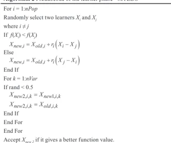
Algorithm 1 Pseudocode of the learner phase - TLBO For i = 1:nPop

Randomly select two learners Xi and Xj

where i ≠ j If f(Xi) < f(Xj) X_{new i,} =X_{old i,} +r X_i

(

_i−X_j

)

Else X_{new i}, =X_{old i}, +r X_i

(

_j−X_i

)

End If End For

Accept Xnew if it gives a better function value.

of the current solutions (dimensions) are changed in the MTLBO. It makes better exploitation in the search spaces and gets more diversity. The modified learner phase can be stated as Algorithm 2.

4 Numerical studies

The efficacy of the proposed MTLBO algorithm is compa- red with other evolutionary optimization algorithms includ-ing GA, PSO, ABC, and DE algorithms for different basic benchmark optimization functions. Then, the performance of the MTLBO algorithm is compared with the basic TLBO algorithm for CEC-2005 benchmark optimization functions. In the end, the MTLBO is developed for the optimal design of TMD parameters and optimal tuning of the feedback gain matrix of the controller in an active tendon system.

4.1 Benchmark optimization function

Six benchmark optimization functions as multimodal problems are chosen to test the ability of the global search of different optimization algorithms. The benchmark opti-mization functions are summarized in Table 1.

4.1.1 Experiments A

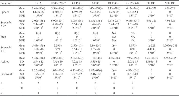
The efficacy of the MTLBO algorithm in comparison with OEA, HPSO-TVAC, CLPSO, APSO, OLPSO-L, OLPSO-G for the benchmark optimization functions, defined in Table 1, are summarized in Table 2. For this purpose, the mean and the standard deviation (SD) crite-ria are inserted in this table. The results of OEA, HPSO-TVAC, CLPSO, and APSO, OLPSO-L, OLPSO-G are reported in [25]. For a fair comparison, the numbers of population (NPop) for TLBO and MTLBO are considered as 5 and the maximum iteration is considered as 5000. 10 runs are assigned for these computations. The number of function evaluations (NFE) for each function is mentioned in the table. Also, the final performance of the MTLBO respect to other algorithms is reported in the last three rows of the Table in terms of worse, better and similar per-formance. "−", "+", and "≈" denote that the performance of the corresponding algorithm is worse than, better than, and similar to that of MTLBO, respectively. NA is used for Not Available. The results show that the MTLBO per-forms better than OEA, HPSO-TVAC, CLPSO, APSO, OLPSO-L and OLPSO-G for all test functions. For most problems, the results are given with less NFE than other algorithms. Similar results are given by the original TLBO and the MTLBO for the most test functions.

Algorithm 2 Pseudocode of the learner phase - MTLBO For i = 1:nPop

Randomly select two learners Xi and Xj

where i ≠ j If f(Xi) < f(Xj) X_{new i,} =X_{old i,} +r X_i

(

_i−X_j

)

Else X_{new i}, =X_{old i}, +r X_i

(

_j−X_i

)

End If For k = 1:nVar If rand < 0.5 X_{new i k}2, , =X_{new i k}1, , X_{new i k}2, , =X_{old i k}, , End If End For End For

Accept Xnew 2 if it gives a better function value.

Where nVar is the number of variables.

Table 1 Benchmark test functions

Test function Formulation Search range Minimum value

Sphere [-100,100]D ₀ Schwefel 2.22 [-10,10]D ₀ Step [-100,100]D ₀ Schwefel 1.2 [-100,100]D ₀ Ackley [-32,32]D ₀ Griewank [-600,600]D ₀ f x x_i i D 1 2 1 ( )= =

∑

f x x_i x i D i i D 2 1 1 ( )= + = =

∑

∏

f x

_i

x

i D 3 2 1

0 5

( )

=

∑

₌

_

+

.

_

f x x_j j i i D 4 1 2 1 ( )=    ₌ _ =

∑

∑

f x D i xi D x D i i D 5 2 1 1 20 0 2 1 1 2 ( )= − −      − _

(

)

= =

∑

∑

exp . * exp cos π 

  + +20 e f x x x i i i D _i i D 6 2 1 1 4000 1 ( )= −       + =

∑

∏

cos

Table 2 Performance of MTLBO, OEA, HPSO-TVAC, CLPSO, APSO, OLPSO-L and OLPSO-G

Function OEA HPSO-TVAC CLPSO APSO OLPSO-L OLPSO-G TLBO MTLBO

Sphere MeanSD NFE 2.48e-30(-) 1.128e-29 1.5*105 3.38e-41(-) 8.50e-41 1.5*105 1.89e-19(-) 1.49e-19 1.5*105 1.45e-150(-) 5.73e-150 1.5*105 1.11e-38(-) 1.28e-28 1.5*105 4.12e-54(-) 6.34e-54 1.5*105 4.9e-321 0 5*104 4.9e-321 0 5*104 Schwefel 2.22 Mean SD NFE 2.07e-13(-) 2.44e-12 2.0*105 6.92e-23(-) 6.89e-23 2.0*105 1.01e-13(-) 6.54e-14 2.0*105 5.15e-84(-) 1.44e-83 2.0*105 7.67e-22(-) 5.63e-22 2.0*105 9.85e-30(-) 1.01e-29 2.0*105 4.9e-321 0 5*104 4.9e-321 0 5*104 Step MeanSD NFE 0(~) 0 1.0*105 0(~) 0 1.0*105 0(~) 0 1.0*105 0(~) 0 1.0*105 NA NA NA NA NA NA 0 0 5*104 0 0 5*104 Schwefel 1.2 Mean SD NFE 5.43e-17(-) 1.68e-16 1.0*105 2.39(-) 3.71 1.0*105 2.57e-1(-) 6.64e-11 1.0*105 5.8e-15(-) 1.01e-14 1.0*105 0(~) 0 1.0*105 1.07(-) 0.99 1.0*105 1e-323 4.4238 5*104 9.2076e-281 0 5*104 Ackley MeanSD NFE 5.34e-14(-) 2.94e-13 5.0*104 2.06e-10(-) 9.45e-10 5.0*104 2.01e-12(-) 9.22e-13 5.0*104 1.11e-14(-) 3.55e-15 5.0*104 4.14e-5(-) 0 5.0*104 7.98e-15(-) 2.03e-15 5.0*104 4.2633e-15 1.498e-15 5*104 3.5527e-15 0 5*104 Griewank MeanSD NFE 1.32e-02(-) 1.56e-02 5*104 1.07e-02(-) 1.14e-02 5*104 6.45e-13(-) 2.07e-12 5*104 1.67e-02(-) 2.41e-02 5*104 0(~) 0 5*104 4.83e-03(-) 8.63e-03 5*104 0 0 5*104 0 0 5*104 + 5 5 5 5 3 5 1 − 0 0 0 0 0 0 1 ≈ 1 1 1 1 2 0 4 4.1.2 Experiments B

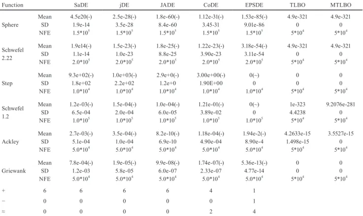
The experiments of this group compare the performance of the MTLBO algorithm with those given by SaDE, jDE, JADE, CoDE, EPSDE for the benchmark functions described in Table 1. The results of these algorithms are directly taken from [25]. The results are inserted in Table 3. A similar result is obtained for this experiment. The superiority of the MTLBO than other algorithms are observed.

4.1.3 Experiments C

The experiments of this group validate the performance of the MTLBO algorithm in comparison with CABC, GABC, RABC and IABC for solving the mentioned six benchmark optimization functions. The results of these algorithms are given by [25]. The corresponding results for each test function are shown in Table 4. Similar to the results in experiments A and B, it is found that the MTLBO performs better than other optimization algo-rithms to find the best solution for the mentioned bench-mark test functions.

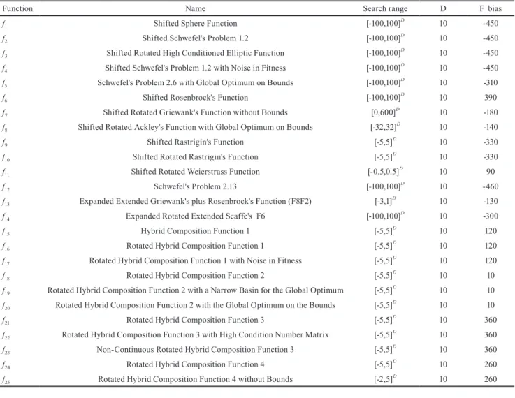
4.1.4 CEC-2005 benchmark optimization functions

In Tables 2–4, the optimal result of each function is zero and it is concluded that both basic TLBO and the MTLBO give better performance than other algorithms in terms of mean and SD.

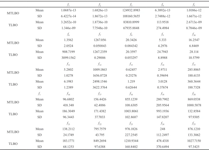
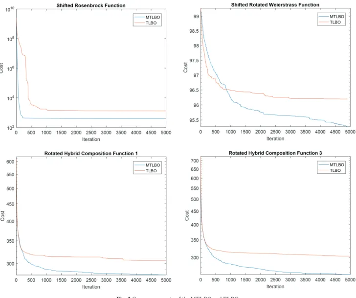
Also, it is found that the basic TLBO and MTLBO result in the same results in most benchmark optimization func-tions. Considering different CEC-2005 benchmark optimi-zation functions that have the non-zero optimal result, a comparison between the performance of the MTLBO and TLBO is interesting. Table 5 shows the CEC-2005 bench-mark optimization functions. For a fair comparison, the number of runs is considered as 25 and the number of func-tion evaluafunc-tions is 10000*D where D is dimensionalities of the problems. Also, the population sizes for both TLBO and MTLBO are considered as 10. The average error for 25 functions is indicated in Table 6. Also, the convergence rate diagrams for functions 1, 6, 11, 16, and 21 are illustrated in Fig. 2. In Table 6, it can be seen that the MTLBO has a less mean of error than conventional TLBO in all functions except functions 3 and 20. Furthermore, Fig. 2 shows that the MTLBO converges more quickly than the TLBO to the optimal solutions. Consequently, the MTLBO gives better performance and reliable results than the TLBO.

4.2 Engineering optimization problems

The performance of the MTLBO algorithm is also verified for some engineering optimization problems. Four bench-mark engineering problems are selected for this purpose and the penalty function method approach is utilized to handle the defined constraints for the problems as the fol-lowing pseudo-cost function:

Table 3 Performance of MTLBO, JADE, jDE, SaDE, CoDE, and EPSDE

Function SaDE jDE JADE CoDE EPSDE TLBO MTLBO

Sphere Mean SD NFE 4.5e20(-) 1.9e-14 1.5*105 2.5e-28(-) 3.5e-28 1.5*105 1.8e-60(-) 8.4e-60 1.5*105 1.12e-31(-) 3.45-31 1.5*105 1.53e-85(-) 9.01e-86 1.5*105 4.9e-321 0 5*104 4.9e-321 0 5*104 Schwefel 2.22 Mean SD NFE 1.9e14(-) 1.1e-14 2.0*105 1.5e-23(-) 1.0e-23 2.0*105 1.8e-25(-) 8.8e-25 2.0*105 1.22e-23(-) 3.90e-23 2.0*105 3.18e-54(-) 3.11e-54 2.0*105 4.9e-321 0 5*104 4.9e-321 0 5*104 Step Mean SD NFE 9.3e+02(-) 1.8e+02 1.0*104 1.0e+03(-) 2.2e+02 1.0*104 2.9e+0(-) 1.2e+0 1.0*104 3.00e+00(-) 1.90E+00 1.0*104 0(~) 0 1.0*104 0 0 5*104 0 0 5*104 Schwefel 1.2 Mean SD NFE 1.2e-03(-) 6.5e-04 1.0*105 1.5e-04(-) 2.0e-04 1.0*105 1.0e-04(-) 6.0e-05 1.0*105 1.21e-01(-) 3.89e-02 1.0*105 0(~) 0 1.0*105 1e-323 4.4238 5*104 9.2076e-281 0 5*104 Ackley Mean SD NFE 2.7e-03(-) 5.1e-04 5.0*104 3.5e-04(-) 1.0e-04 5.0*104 8.2e-10(-) 6.9e-10 5.0*104 1.18e-04(-) 4.90e-04 5.0*104 1.94e-2(-) 8.90e-4 5.0*104 4.2633e-15 1.498e-15 5*104 3.5527e-15 0 5*104 Griewank MeanSD NFE 7.8e-04(-) 1.2e-03 5.0*104 1.9e-05(-) 5.8e-05 5.0*104 9.9e-08(-) 6.0e-07 5.0*104 1.74e-07(-) 2.33e-07 5.0*104 5.36e-13(-) 4.77e-14 5.0*104 0 0 5*104 0 0 5*104 + 6 6 6 6 4 1 − 0 0 0 0 0 1 ≈ 0 0 0 0 2 4

Table 4 Performance of MTLBO, CABC, GABC, RABC, and IABC

Function CABC GABC RABC IABC TLBO MTLBO

Sphere MeanSD NFE 2.3e-40(-) 1.7e-40 1.5*105 3.6e-63(-) 5.7e-63 1.5*105 9.1e-61(-) 2.1e-60 1.5*105 5.34e-178(-) 0 1.5*105 4.9e-321 0 5*104 4.9e-321 0 5*104 Schwefel 2.22 Mean SD NFE 3.5e-30(-) 4.8e-30 2.0*105 4.8e-45(-) 1.4e-45 2.0*105 3.2e-74(-) 2.0e-73 2.0*105 8.82e-127(-) 3.49e-126 2.0*105 4.9e-321 0 5*104 4.9e-321 0 5*104 Step MeanSD NFE 0(~) 0 1.0*104 0(~) 0 1.0*104 0(~) 0 1.0*104 0(~) 0 1.0*104 0 0 5*104 0 0 5*104 Schwefel 1.2 Mean SD NFE 1.3e-00(-) 2.7e-00 1.0*105 1.5e-10(-) 2.7e-10 1.0*105 2.3e-02(-) 5.1e-01 1.0*105 0(~) 0 1.0*105 1e-323 4.4238 5*104 9.2076e-281 0 5*104 Ackley MeanSD NFE 1.0e-05(-) 2.4e-06 5.0*104 1.8e-09(-) 7.7e-10 5.0*104 9.6e-07(-) 8.3e-07 5.0*104 3.87e-14(-) 8.52e-15 5.0*104 4.2633e-15 1.498e-15 5*104 3.5527e-15 0 5*104 Griewank Mean SD NFE 1.2e-04(-) 4.6e-04 5.0*104 6.0e-13(-) 7.7e-13 5.0*104 8.7e-08(-) 2.1e-08 5.0*104 0(~) 0 5.0*104 0 0 5*104 0 0 5*104 + 5 5 5 3 1 − 0 0 0 0 0 ≈ 1 1 1 3 5

Table 5 CEC-2005 Benchmark test functions

Function Name Search range D F_bias

f1 Shifted Sphere Function [-100,100]D 10 -450

f2 Shifted Schwefel's Problem 1.2 [-100,100]D 10 -450

f3 Shifted Rotated High Conditioned Elliptic Function [-100,100]D 10 -450

f4 Shifted Schwefel's Problem 1.2 with Noise in Fitness [-100,100]D 10 -450

f5 Schwefel's Problem 2.6 with Global Optimum on Bounds [-100,100]D 10 -310

f6 Shifted Rosenbrock's Function [-100,100]D 10 390

f7 Shifted Rotated Griewank's Function without Bounds [0,600]D 10 -180

f8 Shifted Rotated Ackley's Function with Global Optimum on Bounds [-32,32]D 10 -140

f9 Shifted Rastrigin's Function [-5,5]D 10 -330

f10 Shifted Rotated Rastrigin's Function [-5,5]D 10 -330

f11 Shifted Rotated Weierstrass Function [-0.5,0.5]D 10 90

f12 Schwefel's Problem 2.13 [-100,100]D 10 -460

f13 Expanded Extended Griewank's plus Rosenbrock's Function (F8F2) [-3,1]D 10 -130

f14 Expanded Rotated Extended Scaffe's F6 [-100,100]D 10 -300

f15 Hybrid Composition Function 1 [-5,5]D 10 120

f16 Rotated Hybrid Composition Function 1 [-5,5]D 10 120

f17 Rotated Hybrid Composition Function 1 with Noise in Fitness [-5,5]D 10 120

f18 Rotated Hybrid Composition Function 2 [-5,5]D 10 10

f19 Rotated Hybrid Composition Function 2 with a Narrow Basin for the Global Optimum [-5,5]D 10 10 f20 Rotated Hybrid Composition Function 2 with the Global Optimum on the Bounds [-5,5]D 10 10

f21 Rotated Hybrid Composition Function 3 [-5,5]D 10 360

f22 Rotated Hybrid Composition Function 3 with High Condition Number Matrix [-5,5]D 10 360

f23 Non-Continuous Rotated Hybrid Composition Function 3 [-5,5]D 10 360

f24 Rotated Hybrid Composition Function 4 [-5,5]D 10 260

f25 Rotated Hybrid Composition Function 4 without Bounds [-2,5]D 10 260

f X W X max g X cost k n k

{ }

( )

= +

(

)

( )

{ }

= 

( )

{ }

  =

∑

1 0 1 1 2 ε ϑ ϑ ε * * , , , (4)

where, W({X}), gk({X}) and ϑ are the cost function, the

constraint, and the total constraint violation of the optimi-zation problem, respectively. The constants ε1 and ε2 are

selected based on the exploration and exploitation rates of the search space. In the present work, ε1 = 1 and ε2 is

changed from 1.5 to 3.

4.2.1 Tension/compression spring design

This problem aims to minimize the weight of the tension/ compression spring shown in Fig. 3. The problem has three design variables including the wire diameter (d), the mean diameter of coil (D), and the number of active coils (N). It is subjected to three nonlinear inequality constraints in terms of shear stress, surge frequency, and deflection and one linear inequality constraint as follows:

Minimze: Subject to: f x x x x g x x x x g

( )

=

(

+

)

( )

= − ≤ 3 2 1 2 1 2 3 3 1 4 2 1 71785 0 2 2 2 2 1 2 2 1 3 1 4 1 2 3 4 12566 1 5108 1 0 1 140 45 x x x x x x x x g x

( )

= − −

(

)

+ − ≤

( )

= − . xx x x g x x x x x 1 2 2 3 4 1 2 1 2 0 1 5 1 0 0 05 2 00 0 25 1 30 ≤

( )

= + − ≤ ≤ ≤ ≤ ≤ . . . , . . where ,, and 2 00. ≤x₃≤15 00. (5)

The tension/compression spring design problem has been undergone under co-evolutionary DE (CDE) [26], ABC [27], CPSO [28] and HPSO [29]. The convergence histories of the original TLBO and MTLBO for the opti-mization problem are shown in Fig. 4.

Table 7 presents the details of the best solutions using the basic TLBO and MTLBO algorithms. The number of population for both TLBO and MTLBO is considered as 10. Table 8 also compared the statistical results of the considered algorithms with those given by the basic TLBO and MTLBO algorithms. Based on the values of the mean and the standard deviation (SD) inserted in Table 8, it can be found that the MTLBO has outperformed the other algorithm. With far fewer NFE adopted for the TLBO and MTLBO compared to other optimization algorithms, the best results are given for both optimization algorithms. It is worth noting that the performance of MTLBO is slightly better than the TLBO in terms of mean, worst and SD criteria.

4.2.2 Optimal design of welded beam

The purpose of the problem is to optimally design a welded beam under certain constraints having minimum cost. The welded beam structure is illustrated in Fig. 5.

As illustrated in the figure, the beam A is welded to the member B. The optimization problem aims to find the

minimum fabrication cost. The design variables are x1, x2,

x3, x4. The constraints of the problem included shear stress

(τ), bending stress of the beam (σ), buckling load on the bar (Pc), and the end deflection of the beam (δ). The

optimiza-tion problem can be formulated as: Minimize: f x

( )

=1 10471x x1 +0 04811x x

(

14 0+x

)

2 2 3 4 2 . . . Subject to: g x1

( )

=τ

( )

x −13600≤0 g x2

( )

=σ

( )

x −30000≤0 g x3

( )

=x_x−x4≤0 g x4 x1 x x x 2 3 4 2 0 10471 0 04811 14 5 0 0

( )

=

(

.

)

+ .

(

+

)

− . ≤ g x5

( )

=0 125. − ≤x1 0 g x6

( )

=δ

( )

x −0 25. ≤0 g x7

( )

=6000−p x_c

( )

≤0

Table 6 The average error for CEC-2005 benchmark functions

f1 f2 f3 f4 f5

MTLBO Mean 1.0687e-13 1.6826e-13 124932.8983 6.3892e-13 1.0186e-12

SD 6.4227e-14 1.8672e-13 108160.5655 2.7488e-12 1.6671e-12

TLBO Mean 3.2652e-10 1.8736e-10 83810.8999 113.9518 2.6713e-09

SD 1.346e-09 7.7548e-10 67935.8848 274.4984 8.7846e-09

f6 f7 f8 f9 f10 MTLBO Mean 1.3562 1267.056 20.3426 5.333 16.2547 SD 2.0524 0.050043 0.084342 4.2976 6.8469 TLBO Mean 908.7199 1267.2359 20.3597 24.7943 28.114 SD 3099.1562 0.29006 0.053297 8.8988 10.5799 f11 f12 f13 f14 f15 MTLBO Mean 5.2802 1009.1863 0.62457 2.9711 285.8865 SD 1.0278 1656.0728 0.25276 0.39694 188.6135 TLBO Mean 6.1983 2498.1546 1.219 3.0128 360.3644 SD 1.2389 3622.3764 0.62644 0.37674 188.7328 f1 f16 f17 f18 f19 f20 MTLBO Mean 96.6802 156.4426 855.1239 280.7902 869.0538 SD 418.348 62.4886 108.6305 205.9564 1000.5878 TLBO Mean 186.3049 171.4382 1003.8061 993.1936 132.8584 SD 96.3443 37.7033 102.8687 147.8207 97.9305 f21 f22 f23 f24 f25 MTLBO Mean 138.2112 795.7579 976.1826 248 876.1210 SD 24.1749 43.795 227.2545 112.2497 133.3062 TLBO Mean 183.1771 849.2694 1210.9344 478.4318 1027.7150 SD 68.1253 97.6388 160.8402 370.6494 97.3425

where: τ x τ τ τ x τ R

( )

=

( )

′2+

(

₂ ′ ′′

)

2 +

( )

′′2 2 ′ = τ 6000 2x x1 2 ′′ = τ MR J M =  +x      6000 14 2 2 R= x +x x+   _ 2 2 1 3 2 4 2 J= x x x +x x+                      2 2 12 2 1 2 2 2 1 3 2 σ x x x

( )

=504000 4 3 2 δ x x x

( )

=

(

30 1065856000* 6

)

_{4 3}3 p x x x x c

( )

=

(

)

−

(

)

       4 013 30 10 36 196 1 30 10 4 12 10 28 6 3 2 4 6 3 6 6 . * * *          ≤ ≤ ≤ ≤ 0 1. x x₁, ₄ 2 0. , and 0 1. x x₂, ₃ 10 0. . (6)

The welded beam optimization design problem has been investigated using the modified differential evolution algo-rithm (COMDE) [32], ABC [27], hybrid PSO with differen-tial evolution (PSO-DE) [33], co-evolutionary PSO (CPSO)

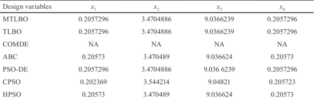
[28] and hybrid PSO (HPSO) [29]. Considering the number of population nPop = 10 for the basic TLBO and TLBO algorithms, the convergence graphs and optimal parame-ters of the problem are shown in Fig. 6 and Table 9, respec-tively. Furthermore, a compression among the statistical results of the considered algorithms with those given by the basic TLBO and MTLBO is indicated in Table 10.

Table 10 confirms the capability of the MTLBO, TLBO, and COMDE to find the optimal solution in all runs. It is evident that the MTLBO has lower values of SD than COMDE, but it has the same mean and NFE with COMDE. Considering a smaller NFE for the MTLBO than the other algorithms, it gives better performance than all other algo-rithms according to the values of the mean and SD. Also, Fig. 6 shows that the MTLBO converges more rapidly than the original TLBO to the optimal solution.

4.2.3 A reinforced concrete beam design

Fig. 7 shows a simplified total cost optimization problem for A 30-ft simple reinforced concrete beam introduced by Amir and Hasegawa [34]. It is subjected to a live load of 2.0 klbf and a dead load (including the weight of the

Fig. 5 The optimal design problem of the welded beam [31]

Table 8 The statistical results of the tension/compression spring optimization design problem

Method Best Mean Worst SD NFE

MTLBO 0.012666 0.012686 0.012754 1.9189e-05 20000 TLBO 0.012665 0.012696 0.012791 2.8982e-05 20000 ABC 0.012665 0.012709 NA 1.28 e-02 30000 CDE 0.0126702 0.012703 0.012790 2.7 e-05 240000 CPSO 0.0126747 0.012730 0.012924 5.20 e-05 200000 HPSO 0.0126652 0.012707 0.012719 1.58 e-05 81000

Fig. 4 Convergence graphs for tension/compression spring design problem

Fig. 3 The tension/compression spring design problem [30]

Table 7 Optimal solutions for the tension/compression spring design problem Design variables x1 x2 x3 MTLBO 0.052351 0.372865 10.407740 TLBO 0.051565 0.353759 11.464504 ABC 0.051749 0.358179 11.203763 CDE 0.051609 0.354714 11.410831 CPSO 0.051728 0.357644 11.244543 HPSO 0.051706 0.357126 11.265083

beam) of 1.0 klbf. The concrete compressive strength (Fc)

and yield stress of the reinforcing steel (Fy) are considered

as 5 ksi, and 50 ksi, respectively. The unit costs of con-crete and steel are $0.02/in2_{/linear ft and $1.0/in}2_{/linear ft,}

respectively. The design variables are the area of the rein-forcement (As), the width of the beam (b), and the depth of

the beam (h). The cross-sectional area of the bar as a dis-crete variable is selected from the standard bar dimensions reported in [34], while the width of the concrete beam and the depth of the beam are respectively integer and contin-uous design variables. The effective depth is considered as 0.8x2. The structure should meet the required strength

according to ACI 318-77 building code as follows:

M A h A bh M M u s y s y c a l =

(

)

 −      ≥ + 0 9 0 8 1 0 0 59 0 8 1 4 1 7 . . . . . . . . σ σ σ (7)

In which Mu, Ma, and Ml are the moments of the beam

under the flexural strength, dead load, and live load, respec-tively. In this case, the values of Md and Ml are 1,350 kip-in

2,700 kip-in, respectively. The depth to width ratio is restricted to 4 or less. The optimization problem can be defined as the following formulation:

Minimize: Subject to: f A b h A bh g b h h b g A s s s , , . . ,

(

)

= +

( )

= − ≤ 2 9 0 6 4 0 1 2 ,, ,b h . . A bs A hs

(

)

=180+7 375 − ≤0 2 (8)

The variables bound of the cross-sectional area of the reinforcing bar, the width of the beam and the depth of the beam are {6.0, 6.16, 6.32, 6.6, 7.0, 7.11, 7.2, 7.8, 7.9, 8.0, 8.4} in2_{, {28, 29, 30, 31, …, 38, 39, 40} in and 5 ≤ h ≤ 10 in,}

respectively. The functions g1 and g2, are the constrained

functions derived by Liebman et al. [36].

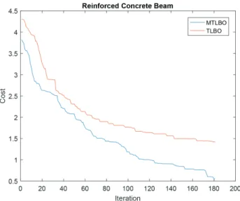
The problem has been also assessment through Hybrid discrete steepest descent and rotating coordinate direc-tions methods (SD-RC) [34], Generalized Hopfield net-work-based augmented Lagrange multiplier approach (GHN-ALM) [37], GHN based extended penalty approach (GHN-EP) [37], Adaptive hybrid GA with fuzzy logic con-troller (FLC-AHGA) [38]. Fig. 8 indicates the convergence graphs for the optimal design of the reinforced concrete beam. Also, Table 11 presents the optimal solutions and the statistical results of the problem by the above-mentioned

Table 9 Optimal solutions for the welded beam optimization design problem

Design variables x1 x2 x3 x4 MTLBO 0.2057296 3.4704886 9.0366239 0.2057296 TLBO 0.2057296 3.4704886 9.0366239 0.2057296 COMDE NA NA NA NA ABC 0.20573 3.470489 9.036624 0.20573 PSO-DE 0.2057296 3.4704886 9.036 6239 0.2057296 CPSO 0.202369 3.544214 9.04821 0.205723 HPSO 0.20573 3.470489 9.036624 0.20573

NA is used for not available.

Table 10 The statistical results of the welded beam optimization design problem

Method Best Mean Worst SD NFE

MTLBO 1.7248523 1.7248523 1.7248523 1.1362e-15 20000 TLBO 1.7248523 1.7248523 1.7248523 2.5007e-14 20000 COMDE 1.7248523 1.7248523 1.7248523 1.60 e-12 20000 ABC 1.724852 1.741913 NA 3.1 e-02 30000 PSO-DE 1.724853 1.724858 1.724881 4.1 e-06 33000 CPSO 1.728024 1.748831 1.782143 1.29 e-02 200000 HPSO 1.724852 1.749040 1.814295 4.00 e-02 81000

NA is used for not available.

optimization algorithms. The number of population for the basic TLBO and MTLBO is adopted as 25. Table 11 shows that the MTLBO with the lowest values of Mean, SD respect to other algorithms, provides an efficient, qual-ified and robust method to find the optimal design of the reinforced concrete beam.

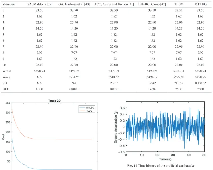
4.2.4 Ten-bar truss design using discrete variables

Another example is the optimal design of a ten-bar truss, shown in Fig. 9. A set of 41 discrete values for possible cross-sectional areas of the members is selected as (1.62, 1.80, 1.99, 2.13, 2.38, 2.62, 2.88, 2.93, 3.09, 3.13, 3.38, 3.47, 3.55, 3.63, 3.84, 3.87, 3.88, 4.18, 4.22, 4.49, 4.59, 4.80, 4.97, 5.12, 5.74, 7.22, 7.97, 11.5, 13.5, 13.9, 14.2, 15.5, 16.0, 16.9, 18.8, 19.9, 22.0, 22.9, 26.5, 30.0, and 33.5 in2_{). The}

maxi-mum allowable stress of the truss members is restricted to

±25 ksi while the maximum vertical and horizontal deflec-tion of the nodes is ±2.0 in. The unit weight of the mate-rial was 0.1 lb/in3 _{and its elasticity modulus is considered}

as 107 psi. GA (Mahfouz) [39], GA (Barbosa et al.) [40], ACO (Camp and Bichon) [41], and BB–BC (Camp) [42] has investigated the problem. Table 12 indicates the sta-tistical results of considered algorithms along with details of the best solutions. It is found that the best design is given by the MTLBO algorithm in which the weight of truss was obtained as 5490.75 lb. The convergence graphs for the optimal design of the ten-bar truss design are also illustrated in Fig. 10. The mean weight of the best fea-sible truss designs was 5490.74 lb which is resulted in a standard deviation of 0.13852 lb. after 50 runs of the algo-rithm with the number of a population of 25. The number of truss analyses needed by the MTLBO algorithm to be converged was 7500. In comparison with GA, ACO, and BB–BC algorithms, the MTLBO algorithm requires less computational effort to find the optimal design. For the truss design problem with ten design variables, a compar-ison between the results given by the MTLBO with those given for other algorithms is remarkable. The standard deviation of the MTLBO is 0.14, whereas the correspond-ing values for other algorithms are about 23, 12 and 212, respectively. Therefore, it is concluded that the superiority of the MTLBO is evident for optimization problems with a large number of design variables.

4.3 Control optimization problems

Two structural control problems are addressed in this sec-tion to validate the proposed MTLBO algorithm. The first problem is the optimal design of TMD as a passive control device for the seismic-excited structure. The second prob-lem is to tune the feedback gain matrix of a controller in a structure equipped with an active tendon system (ATS).

Fig. 8 Convergence graphs for the optimal design of the reinforced concrete beam

Table 11 Optimal solutions and statistical results of the reinforced concrete beam design problem

Optimal solution of the

design variable The statistical results

Method As b h Mean SD NFE

MTLBO 6.32 34 8.50 359.8099 1.0511 10000 TLBO 6.6 33 8.50 361.5814 1.8981 10000 SD-RC 7.8 31 7.79 374.2 NA 10000 GHN-ALM 6.6 33 8.495227 374.2 NA 10000 GHN-EP 6.32 34 8.637180 362.00648 NA 10000 GA 7.20 32 8.0451 366.1459 NA 10000 FLC-AHGA 6.16 35 8.7500 364.8541 NA 10000

NA is used for not available.

4.3.1 Optimal design of tuned mass damper parameters

The optimal design of a Tuned mass damper (TMD) located on the top story of a ten-story shear building subjected to the artificial earthquake excitation, shown in Fig. 11, is considered for validation of the proposed MTLBO algo-rithm. The artificial earthquake is produced by a band-lim-ited Gaussian white noise with the following power spec-tral density function:

s g g g g g ω ξ ω ω ω ξ ω ω ω

( )

= + +         4 2 2 2 , (9)

where ξg and ωg are the ground damping and frequency,

respectively. For numerical simulations, the ground damp-ing and frequency are adopted as 0.3 and 2π rad/s, respec-tively [44].

The mass, damping coefficient, and stiffness coefficient of each story are 360 ton, 6.2 MNs/m, and 650 MN/m, respectively. The optimization problem aims to find the opti-mal TMD parameters, including TMD mass (md), damping

coefficient (cd) and stiffness coefficient (kd), for minimizing

the maximum top story displacement as follows:

Minimize Subject to: and I max x t max x t m c k t t d d d =

( )

( ) ≤ ≤ ≤ 108, 1000, 55000 150 max_t xTMD

( )

t −xtop

( )

t cm, (10)

where I is the maximum floor displacement of the structure with the TMD normalized to the corresponding response for the structure without TMD. A limitation for the maxi-mum TMD stroke is added to the problem as a constrained. In other words, the term of max_t||x_TMD(t) – x_top(t)|| refers to

Fig. 10 Convergence graphs for the optimal design of Ten-bar truss design

Fig. 11 Time history of the artificial earthquake

Table 12 The best solutions and the statistical results of the Ten-bar truss design problem

Members GA, Mahfouz [39] GA, Barbosa et al [40] ACO, Camp and Bichon [41] BB–BC, Camp [42] TLBO MTLBO

1 33.50 33.50 33.50 33.50 33.50 33.50 2 1.62 1.62 1.62 1.62 1.62 1.62 3 22.90 22.90 22.90 22.90 22.90 22.90 4 14.20 14.20 14.20 14.20 14.20 14.20 5 1.62 1.62 1.62 1.62 1.62 1.62 6 1.62 1.62 1.62 1.62 1.62 1.62 7 22.90 22.90 22.90 22.90 22.90 22.90 8 7.97 7.97 7.97 7.97 7.97 7.97 9 1.62 1.62 1.62 1.62 1.62 1.62 10 22.00 22.00 22.00 22.00 22.00 22.00 Wmin 5490.74 5490.74 5490.74 5490.74 5490.74 5490.74 Wavg NA 5534.98 5510.52 5494.17 5595.60 5490.75 SD NA NA 23.19 12.42 211.55 0.13852 NFE 8000 200000 10000 8694 7500 7500

the maximum relative TMD displacement respect to the maximum roof displacement which should be less than 150 cm. Using a penalty method, the complicated con-strained optimization problem can be converted to an unconstrained optimization problem as follows:

J I x t x t t TMD Roof = × +

(

(

[ ]

)

)

=

( )

−

( )

− 1 50 0 150 1 max , max . α α (11) For a population number of 10, the mean, best, worst, and SD results for 30 runs are inserted in Table 13. The convergence graphs for both TLBO and MTLBO are illus-trated in Fig. 12. Furthermore, the optimal parameters of the TMD using the TLBO and MTLBO are inserted in Table 14. Some optimal design scenarios for the men-tioned problem reported by GA in [7], Lee et al. [45] and charged system search (CSS) in [9], are also inserted in the Table for comparison purposes.

The maximum seismic responses of the structure sub-jected to the El Centro (1940) NS earthquake in terms of

maximum floor displacement and acceleration are shown

in Tables 15 and 16, respectively. The optimized TMD by TLBO and MTLBO gives better results than GA and the results given by Lee et al. in the reduction of structural

responses in terms of floor displacement and accelera -tion. An average reduction of 37.09 % in the maximum

displacement and an average reduction of 29.44 % in the

maximum acceleration of floors are obtained for both

TLBO and MTLBO. However, as found from Table 13, the MTLBO with a less SD provides reliable results than the TLBO. The MTLOB performs better than CSS in the reduction of the maximum floor acceleration, while the CSS results in more reduction in the maximum floor

Table 13 The statistical results of the optimal design problem of TMD

Method Mean Best Worst SD

TLBO 0.484426 0.483998 0.488119 9.227553e-04 MTLBO 0.484277 0.483996 0.485167 2.763895e-04

Fig. 12 Convergence graphs for the optimal design of TMD

Table 14 Optimum TMD parameters for the optimal design problem of TMD

Methods Optimum parameters

md (ton) cd (kNs/m) kd (kN/m) GA [7] 108 151.5 3750 Lee et al. [45] 108 271.79 4126.93 CSS [9] 108 88.697 4207.735 TLBO 107.99 214.81 4119.55 MTLBO 108 214.82 4119.83

Table 15 Maximum displacements of stories subjected to the El Centro (1940) NS earthquake

Maximum displacement (m) Percentage of reduction (%)

Story Without TMD GA [7] Lee et al. [45] CSS [9] TLBO MTLBO GA Lee et al. [45] CSS TLBO MTLBO

1 0.031 0.019 0.020 0.0185 0.019 0.019 38.71 35.48 40.32 38.80 38.80 2 0.060 0.037 0.039 0.0362 0.037 0.037 38.33 35.00 39.67 38.20 38.20 3 0.087 0.058 0.057 0.0525 0.054 0.054 33.33 34.48 39.65 38.10 38.10 4 0.112 0.068 0.073 0.0682 0.069 0.069 39.29 34.82 39.11 38.37 38.37 5 0.133 0.082 0.087 0.0825 0.082 0.082 38.35 34.59 37.97 37.98 37.98 6 0.151 0.094 0.099 0.0950 0.095 0.095 37.75 34.44 37.09 37.33 37.33 7 0.166 0.104 0.108 0.1056 0.105 0.105 37.35 34.94 36.39 36.76 36.76 8 0.177 0.113 0.117 0.1139 0.113 0.113 36.16 33.90 35.65 35.89 35.89 9 0.184 0.119 0.123 0.1196 0.120 0.120 35.33 33.15 35.00 34.95 34.95 10 0.188 0.122 0.126 0.1225 0.123 0.123 35.11 32.98 34.84 34.55 34.55 TMD – 0.358 0.282 0.4933 0.341 0.341 --- --- --- ---Average reduction (%) 36.97 34.38 37.57 37.09 37.09

displacement. It is noted that the results of the CSS are obtained for an unconstraint TMD design problem (with-out the TMD stroke constraint defined in Eq. (13). In other words, the optimal design of the TMD given by CSS does not satisfy the TMD stroke constraint during the artificial earthquake excitation.

4.3.2 Optimal active control design

A three-story building model studied in [46] is considered. An ATS is installed between the first floor and the ground floor. The mass, damping, and stiffness matrices of the model are as follows:

M C s s kg =          

( )

= − − − − 98 3 0 0 0 98 3 0 0 0 98 3 175 50 0 50 100 50 0 5 . . . , 0 0 50 10 12 0 6 84 0 6 84 13 7 6 84 0 6 5          

(

)

= − − − − N sec m s . / , . . . . . . K 8 84 6 84. .                 N m (12)

Considering Z(t) = [x1 x2 x3 ẋ1 ẋ2 ẋ3]T, L and H as the

loca-tion vectors of the control force and ground acceleraloca-tion, the state space form of the equation of motion of the struc-tural model can be stated as:

 _ Z

( )

t =AZ t

( )

+Bu t

( )

+Hx t_g

( )

(13) where A I M K M C B M L = − −         = −  × × − − × − 0 0 3 3 3 3 1 1 3 1 1 s s s s s T , (14)

Considering the cost function defined in Eq. (15), the active control force of the linear-quadratic regulator (LQR) controller is given by Eq. (16).

J t t t dt t T T =

∫

{

( )

( )

+

( )

}

0 Z QZ R u R , (15) u t

_{( )}

_{= −GZ}

_{( )}

t _{= −R B PZ}−1 T

_{( )}

t _{, (16)} where G is a feedback gain matrix of the controller. Also,

Q and R are the symmetric weighting matrices. Further-more, P is a semi-positive definite matrix that can be obtained from the following Riccati equation:

PA A P PBR B P Q+ T − −1 T + =

0. (17)

In the LQR controller, the weighting matrices Q and R

are the design matrices for optimal tuning of the con-trol force. For the problem, the weighting matrices are assumed as the following form:

Q=diag

(

[

α

]

)

R= −β

0 0 1 1 1 , 10 . (18)

The maximum displacement of floors in the controlled structure normalized to the corresponding response in the uncontrolled structure is assumed as a cost function to tune the optimal design variables i.e. α and β. The TLBO and MTLBO algorithms are utilized for optimal tuning of the weighting matrices. For a population of 10, the optimal design and statistical results of the active control design problem for 30 runs are shown in Table 17. The conver-gence graphs for the problem are displayed in Fig. 13. Similar results are obtained for both algorithms, while the MTLBO algorithm resulted in a smaller SD and a higher convergence than rate than the TLBO algorithm. Time his-tories of the top floor displacement, top floor acceleration,

Table 16 Maximum accelerations of stories subjected to the El Centro (1940) NS earthquake

Maximum acceleration (m/s2_{) Percentage of reduction (%)}

Story Without TMD GA [7] Lee et al. [45] CSS [9] TLBO MTLBO GA Lee et al. [45] CSS TLBO MTLBO

1 2.89 2.70 2.67 3.4260 2.66 2.66 6.57 7.61 1.12 8.03 8.03 2 3.97 3.03 3.10 5.2593 3.02 3.02 23.68 21.91 1.47 24.01 24.01 3 4.93 3.53 3.64 5.9736 3.51 3.51 28.40 26.17 2.60 28.90 28.90 4 5.68 3.94 3.99 6.2626 3.88 3.88 30.63 29.75 14.56 31.75 31.75 5 6.14 4.08 4.12 6.3223 4.02 4.02 33.55 32.90 23.59 34.57 34.57 6 6.55 3.83 4.14 6.1456 3.88 3.88 41.53 36.79 30.00 40.81 40.81 7 6.71 4.39 4.26 5.7233 4.30 4.30 34.58 36.51 36.77 35.97 35.97 8 7.01 5.05 4.95 5.5797 4.99 4.99 27.96 29.39 39.72 28.82 28.83 9 7.84 5.53 5.44 5.8272 5.46 5.46 29.46 30.61 38.19 30.38 30.39 10 8.32 5.81 5.72 5.9564 5.73 5.73 30.17 31.25 37.62 31.13 31.13 Average reduction (%) 28.65 28.29 22.56 29.44 29.44

first-floor drift, and control force of the structure subjected to the scaled 1940 El Centro and 1995 Kobe earthquakes are displayed in Figs. 14 and 15, respectively. A significant reduction is shown in the seismic responses of the struc-ture equipped with ATS in comparison with the uncon-trolled ones. The similar results are obtained for the TLBO and MTLBO algorithms.

5 Conclusions

The design problems of the passive and active control devices for the seismic-excited structures can be defined as some of the optimization problems that demand simple, accurate, and fast optimization algorithms. For this pur-pose, a new modified TLBO algorithm, namely MTLBO, is proposed here. In the MTLBO, an extra term was added to the basic TLBO in the both teacher and learner phases. The performance of MTLBO was firstly validated for some unconstrained and constrained engineering bench-marks. To compare the efficiency of the MTLBO, some evolutionary optimization techniques such as PSO, DE, GA, and ABC along with their various variants were con-sidered. Considering the statistical results undertaken for assessing the performance and reliability of optimiza-tion algorithms, it was concluded that the MTLBO was able to give reliable and better results than other algo-rithms. Furthermore, it was found that the superiority of the MTLBO was evident for optimization problems with a large number of design variables. For some optimization problems, the MTLBO also resulted in the best solution with less function evaluation numbers and computational

Table 17 The optimal design and statistical results of the active control design problem

Method α β Mean Best Worst SD

MTLBO 1 7.475728 0.234946 0.234946 0.234946 7.432602e-14

TLBO 1 7.476714 0.234946 0.234946 0.234954 1.674994e-06

Fig. 13 Convergence graphs for the optimal design of TMD

Fig. 14 Time histories of the top floor displacement, top floor acceleration, first-floor drift and control force of the structure subjected to the El Centro earthquake

efforts rather than other algorithms. Finally, the efficiency of the MTLBO was investigated for the optimal tuning of the parameters in structural engineering problems consisting of passive and active control problems. It was

found that the MTLBO algorithm resulted in faster and better performance than the basic TLBO. Consequently, the MTLBO can be successfully extended and utilized for particular engineering optimization problems.

Fig. 15 Time histories of the top floor displacement, top floor acceleration, first-floor drift and control force of the structure subjected to the Kobe earthquake

References

[1] Etedali, S., Akbari, M., Seifi, M. "MOCS-based optimum design of TMD and FTMD for tall buildings under near-field earthquakes including SSI effects", Soil Dynamics and Earthquake Engineering, 119, pp. 36–50, 2019.

https://doi.org/10.1016/j.soildyn.2018.12.027

[2] Fahimi Farzam, M., Kaveh, A. "Optimum Design of Tuned Mass Dampers Using Colliding Bodies Optimization in Frequency Domain", Iranian Journal of Science and Technology, Transactions of Civil Engineering, 44, pp. 787–802, 2020.

https://doi.org/10.1007/s40996-019-00296-6

[3] Ghasemi, M. R., Shabakhty, N., Enferadi, M. H. "Optimized SMA Dampers in Vibration Control of Jacket-type Offshore Structures (Regular Waves)", International Journal of Coastal and Offshore Engineering, 2(4), pp. 25–35, 2019.

https://doi.org/10.29252/ijcoe.2.4.25

[4] Jarrahi, H., Asadi, A., Khatibinia, M., Etedali, S. "Optimal design of rotational friction dampers for improving seismic performance of inelastic structures", Journal of Building Engineering, 27, Article number: 100960, 2020.

https://doi.org/10.1016/j.jobe.2019.100960

[5] Kaveh, A., Farzam, M. F., Maroofiazar, R. "Comparing H2 and H∞ Algorithms for Optimum Design of Tuned Mass Dampers

under Near-Fault and Far-Fault Earthquake Motions", Periodica Polytechnica Civil Engineering, 64(3), pp. 828–844, 2020.

https://doi.org/10.3311/PPci.16389

[6] Kaveh, A., Fahimi Farzam, M., Hojat Jalali, H., Maroofiazar, R. "Robust optimum design of a tuned mass damper inerter", Acta Mechanica, 231, pp. 3871–3896, 2020.

https://doi.org/10.1007/s00707-020-02720-9

[7] Hadi, M. N. S., Arfiadi, Y. "Optimum Design of Absorber for MDOF Structures", Journal of Structural Engineering, 124(11), pp. 1272– 1280, 1998.

https://doi.org/10.1061/(ASCE)0733-9445(1998)124:11(1272)

[8] Ghasemi, M. R., Varaee, H. "Damping vibration-based IGMM opti-mization algorithm: fast and significant", Soft Computing, 23, pp. 451–481, 2019.

https://doi.org/10.1007/s00500-017-2804-3

[9] Kaveh, A., Mohammadi, S., Khadem Hosseini, O., Keyhani, A., Kalatjari, V. R. "Optimum parameters of tuned mass dampers for seismic applications using charged system search", Iranian Journal of Science and Technology, Transactions of Civil Engineering, 39(C1), pp. 21–40, 2015.

https://doi.org/10.22099/IJSTC.2015.2739

[10] Etedali, S., Zamani, A.-A., Tavakoli, S. "A GBMO-based PIλ_Dμ

controller for vibration mitigation of seismic-excited structures", Automation in Construction, 87, pp. 1–12, 2018.

https://doi.org/10.1016/j.autcon.2017.12.005

[11] Goldberg, D. E. "Genetic Algorithms in Search, Optimization, and Machine Learning", Addison-Wesley Publishing, Boston, MA, USA, 1989.

[12] Kennedy, J., Eberhart, R. "Particle swarm optimization", In: Proceedings of ICNN'95 - International Conference on Neural Networks, Perth, WA, Australia, 1995, pp. 1942–1948.

https://doi.org/10.1109/ICNN.1995.488968

[13] Shabani, A., Asgarian, B., Salido, M., Asil Gharebaghi, S. "Search and rescue optimization algorithm: A new optimization method for solving constrained engineering optimization problems", Expert Systems with Applications, 161, Article number: 113698, 2020.

https://doi.org/10.1016/j.eswa.2020.113698

[14] Varaee, H., Ghasemi, M. R. "Engineering optimization based on ideal gas molecular movement algorithm", Engineering with Computers, 33, pp. 71–93, 2017.

https://doi.org/10.1007/s00366-016-0457-y

[15] Nobahari, M., Ghasemi, M. R., Shabakhty, N. "A novel heuristic search algorithm for optimization with application to structural damage identification", Smart Structures and Systems, 19(4), pp. 449–461, 2017.

https://doi.org/10.12989/sss.2017.19.4.449

[16] Kaveh, A., Kooshkbaghi, M. "Enhanced Artificial Coronary Circulation System Algorithm for Truss Optimization with Multiple Natural Frequency Constraints", Periodica Polytechnica Civil Engineering, 63(2), pp. 362–376, 2019.

https://doi.org/10.3311/PPci.13562

[17] Moez, H., Kaveh, A., Taghizadieh, N. "Natural Forest Regeneration Algorithm for Optimum Design of Truss Structures with Continuous and Discrete Variables", Periodica Polytechnica Civil Engineering, 60(2), pp. 257–267, 2016.

https://doi.org/10.3311/PPci.8884

[18] Kaveh, A., Talatahari, S., Khodadadi, N. "The Hybrid Invasive Weed Optimization-Shuffled Frog-leaping Algorithm Applied to Optimal Design of Frame Structures", Periodica Polytechnica Civil Engineering, 63(3), pp. 882–897, 2019.

https://doi.org/10.3311/PPci.14576

[19] Arzani, H., Kaveh, A., Kamalinejad, M. "Optimal Design of Pitched Roof Rigid Frames with Non-Prismatic Members Using Quantum Evolutionary Algorithm", Periodica Polytechnica Civil Engineering, 63(2), pp. 593–607, 2019.

https://doi.org/10.3311/PPci.14091

[20] Shabani, A., Asgarian, B., Salido, M. "Search and Rescue Optimization Algorithm for Size Optimization of Truss Structures with Discrete Variables", Numerical Methods in Civil Engineering, 3(3), pp. 28–39, 2019. [online] Available at: http://nmce.kntu.ac.ir/ article-1-197-en.html

[21] Rao, R. V., Savsani, V. J., Vakharia, D. P. "Teaching-Learning-Based Optimization: An optimization method for continuous non-linear large scale problems", Information Sciences, 183(1), pp. 1–15, 2012.

https://doi.org/10.1016/j.ins.2011.08.006

[22] Rao, R. V., Savsani, V. J., Vakharia, D. P. "Teaching-learning-based optimization: A novel method for constrained mechanical design optimization problems", Computer-Aided Design, 43(3), pp. 303– 315, 2011.

https://doi.org/10.1016/j.cad.2010.12.015

[23] Nayak, J., Naik, B., Kanungo, D. P., Behera, H. S. "A hybrid elicit teaching learning based optimization with fuzzy c-means (ETLBO-FCM) algorithm for data clustering", Ain Shams Engineering Journal, 9(3), pp. 379–393, 2018.

https://doi.org/10.1016/j.asej.2016.01.010

[24] Dang, M. P., Le, H. G., Chau, N. L., Dao, T.-P. "A multi-objec-tive optimization design for a new linear compliant mechanism", Optimization and Engineering, 21, pp. 673–705, 2020.

https://doi.org/10.1007/s11081-019-09469-8

[25] Satapathy, S. C., Naik, A. "Modified Teaching-Learning-Based Optimization algorithm for global numerical optimization -A com-parative study", Swarm and Evolutionary Computation, 16, pp. 28–37, 2014.

https://doi.org/10.1016/j.swevo.2013.12.005

[26] Huang, F., Wang, L., He, Q. "An effective co-evolutionary differen-tial evolution for constrained optimization", Applied Mathematics and Computation, 186(1), pp. 340–356, 2007.

https://doi.org/10.1016/j.amc.2006.07.105

[27] Akay, B., Karaboga, D. "Artificial bee colony algorithm for large-scale problems and engineering design optimization", Journal of Intelligent Manufacturing, 23, pp. 1001–1014, 2012.

https://doi.org/10.1007/s10845-010-0393-4

[28] He, Q., Wang, L. "A hybrid particle swarm optimization with a feasibility-based rule for constrained optimization", Applied Mathematics and Computation, 186(2), pp. 1407–1422, 2007.

https://doi.org/10.1016/j.amc.2006.07.134

[29] He, Q., Wang, L. "An effective co-evolutionary particle swarm opti-mization for constrained engineering design problems", Engineering Applications of Artificial Intelligence, 20(1), pp. 89–99, 2007.

https://doi.org/10.1016/j.engappai.2006.03.003

[30] Li, G., Shuang, F., Zhao, P., Le, C. "An Improved Butterfly Optimization Algorithm for Engineering Design Problems Using the Cross-Entropy Method", Symmetry, 11(8), Article number: 1049, 2019.

https://doi.org/10.3390/sym11081049

[31] Cagnina, L. C., Esquivel, S. C., Coello, C. A. C. "Solving engi-neering optimization problems with the simple constrained particle swarm optimizer", Informatica, 32(3), pp. 319–326, 2008. [online] Available at: http://www.informatica.si/index.php/informatica/ article/view/204

[32] Mohamed, A. W., Sabry, H. Z. "Constrained optimization based on modified differential evolution algorithm", Information Sciences, 194, pp. 171–208, 2012.

https://doi.org/10.1016/j.ins.2012.01.008

[33] Liu, H., Cai, Z., Wang, Y. "Hybridizing particle swarm optimization with differential evolution for constrained numerical and engineer-ing optimization", Applied Soft Computengineer-ing, 10(2), pp. 629–640, 2010.

https://doi.org/10.1016/j.asoc.2009.08.031

[34] Amir, H. M., Hasegawa, T. "Nonlinear Mixed-Discrete Structural Optimization", Journal of Structural Engineering, 115(3), pp. 626– 646, 1989.

[35] Gandomi, A. H., Yang, X.-S., Alavi, A. H. "Cuckoo search algo-rithm: a metaheuristic approach to solve structural optimization problems", Engineering with Computers, 29, pp. 17–35, 2013.

https://doi.org/10.1007/s00366-011-0241-y

[36] Liebman, J. S., Chanaratna, V., Khachaturian, N. "Discrete struc-tural optimization", Journal of the Strucstruc-tural Division, 107(11), pp. 2177–2197, 1981. [online] Available at: https://cedb.asce.org/ CEDBsearch/record.jsp?dockey=0010542

[37] Shih, C. J., Yang, Y. C. "Generalized Hopfield network based structural optimization using sequential unconstrained minimi-zation technique with additional penalty strategy", Advances in Engineering Software, 33(7–10), pp. 721–729, 2002.

https://doi.org/10.1016/S0965-9978(02)00060-1

[38] Yun, Y. "Study on Adaptive Hybrid Genetic Algorithm and Its Applications to Engineering Design Problems", PhD Dissertation, Waseda University, 2005.

[39] Mahfouz, S. Y. "Design optimization of structural steelwork", PhD Dissertation, University of Bradford, 1999. [online] Available at:

https://ethos.bl.uk/OrderDetails.do?uin=uk.bl.ethos.534650

[40] Barbosa, H. J. C., Lemonge, A. C. C., Borges, C. C. H. "A genetic algorithm encoding for cardinality constraints and automatic vari-able linking in structural optimization", Engineering Structures, 30(12), pp. 3708–3723, 2008.

https://doi.org/10.1016/j.engstruct.2008.06.014

[41] Camp, C. V., Bichon, B. J. "Design of Space Trusses Using Ant Colony Optimization", Journal of Structural Engineering, 130(5), pp. 741–751, 2004.

https://doi.org/10.1061/(ASCE)0733-9445(2004)130:5(741)

[42] Camp, C. V. "Design of Space Trusses Using Big Bang-Big Crunch Optimization", Journal of Structural Engineering, 133(7), pp. 999– 1008, 2007.

https://doi.org/10.1061/(ASCE)0733-9445(2007)133:7(999)

[43] Camp, C. V., Farshchin, M. "Design of space trusses using modi-fied teaching–learning based optimization", Engineering Structures, 62–63, pp. 87–97, 2014.

https://doi.org/10.1016/j.engstruct.2014.01.020

[44] Shourestani, S., Soltani, F., Ghasemi, M., Etedali, S. "SSI effects on seismic behavior of smart base-isolated structures", Geomechanics and Engineering, 14(2), pp. 161–174, 2018.

https://doi.org/10.12989/gae.2018.14.2.161

[45] Lee, C.-L., Chen, Y.-T., Chung, L.-L., Wang, Y.-P. "Optimal design theories and applications of tuned mass dampers", Engineering Structures, 28(1), pp. 43–53, 2006.

https://doi.org/10.1016/j.engstruct.2005.06.023

[46] Asai, T. "Structural control strategies for earthquake response reduction of buildings", PhD Dissertation, University of Illinois at Urbana-Champaign, 2014. [online] Available at: https://www.ide-als.illinois.edu/handle/2142/49571