UNKNOWN AND UNPREDICTABLE ENVIRONMENTS
by
Rayomand Vatcha
A dissertation submitted to the faculty of The University of North Carolina at Charlotte
in partial fulfillment of the requirements for the degree of Doctor of Philosophy in Computing and Information Systems
Charlotte 2012 Approved by: Dr. Jing Xiao Dr. Srinivas Akella Dr. Min Shin Dr. Barry Wilkinson Dr. Jiang Xie
ii
c 2012 Rayomand Vatcha ALL RIGHTS RESERVED
ABSTRACT
RAYOMAND VATCHA. Perceiving guaranteed collision-free robot trajectories in unknown and unpredictable environments. (Under the direction of DR. JING
XIAO)
The dissertation introduces novel approaches for solving a fundamental problem: detecting a collision-free robot trajectory based on sensing in real-world environments that are mostly unknown and unpredictable, i.e., obstacle geometries and their mo-tions are unknown. Such a collision-free trajectory must provide a guarantee of safe robot motion by accounting for robot motion uncertainty and obstacle motion uncer-tainty. Further, as simultaneous planning and execution of robot motion is required to navigate in such environments, the collision-free trajectory must be detected in real-time.
Two novel concepts: (a) dynamic envelopes and (b) atomic obstacles, are intro-duced to perceive if a robot at a configuration q, at a future time t, i.e., at a point
χ = (q, t) in the robot’s configuration-time space (CT space), will be collision-free or not, based on sensor data generated at each sensing moment τ, in real-time. A dynamic envelope detects a collision-free region in the CT space in spite of unknown motions of obstacles. Atomic obstacles are used to represent perceived unknown ob-stacles in the environment at each sensing moment. The robot motion uncertainty is modeled by considering that a robot actually moves in a certain tunnel of a desired trajectory in its CT space. An approach based on dynamic envelopes is presented for detecting if a continuous tunnel of trajectories are guaranteed collision-free in an unpredictable environment, where obstacle motions are unknown. An efficient
iv collision-checker is also developed that can perform fast real-time collision detection between a dynamic envelope and a large number of atomic obstacles in an unknown environment. The effectiveness of these methods is tested for different robots using both simulations and real-world experiments.
v ACKNOWLEDGEMENTS
I am greatly indebted to my advisor, Prof. Jing Xiao, for her patient guidance, advice, and encouragement. Some results in this dissertation would not have been possible without her guidance and feedback. I gratefully acknowledge all the members of my committee who have given their time to read this manuscript and provided valuable advice: Prof. Srinivas Akella, Prof. Min Shin, Prof. Barry Wilkinson, and Prof. Jiang Xie.
I would also like to thank my parents, Soli Minocher Vatcha and Bakhtawar Soli Vatcha, and my sister, Rashna Vatcha, for their love and support.
vi TABLE OF CONTENTS
LIST OF FIGURES ix
CHAPTER 1: INTRODUCTION 1
1.1 Basic tool: C-Space and CT-Space 1
1.2 Different kinds of real-world environments 4
1.3 Planning robot motion 7
1.4 Collision-checking 10
CHAPTER 2: LITERATURE SURVEY 12
2.1 Assumptions made about dynamic environments for robot motion 12 2.2 Extracting information from sensing in unknown environments 14
2.3 Collision detection 18
2.4 Handling motion uncertainty of robot in planning 19
2.5 Limitations 20
CHAPTER 3: RESEARCH OUTLINE 21
3.1 About unknown and unpredictable environments 21 3.2 Online determination of collision-free CT-points via sensing 21
3.3 Detecting safe trajectories for a robot 22
3.4 Outline 23
CHAPTER 4: DYNAMIC ENVELOPE 25
4.1 Robot model 25
4.2 vmax assumption about the environment 26
4.4 Definition and its properties 27 4.5 Collision-free CT-region discovered along with a CT-point 29 4.6 Robustness of approach over exaggerated vmax 33
4.7 Perceived CT-space 35
4.8 Summary 38
CHAPTER 5: DETECTING A COLLISION-FREE TRAJECTORY 40
5.1 Approach 40
5.2 Associating Γ+ to a CT-region of a single CT-point 42 5.3 Associating Γ+ to CT-regions of a set of CT-points 44
5.4 Collision-free perceiver 46
5.5 Implemented examples 48
5.6 Summary 51
CHAPTER 6: ATOMIC OBSTACLES (AO) 54
6.1 Sensor data generated at a sensing moment 54
6.2 Definition, properties and examples 56
6.3 Some free space represented as atomic obstacles 59 6.4 Collision checking between the robot model and obstacles 61
6.5 Summary 62
CHAPTER 7: COLLISION FREE PERCEIVER WITH AO 63
7.1 Extraction and grouping 64
7.2 Hierarchical checking 67
viii
7.4 Algorithm 72
7.5 Time and space coherence 74
7.6 Implementation and experimental results 75
7.7 Summary 79
CHAPTER 8: MOTION PLANNING IN PERCEIVED CT-SPACE 80
8.1 Real-time adaptive motion planner (RAMP) 80
8.2 E-RAMP as practical motion planner 82
8.3 Summary 92
CHAPTER 9: EXPERIMENTS AND RESULTS 94
9.1 Performance data 94
9.2 Simulation environment 95
9.3 Real experiments 103
CHAPTER 10: CONCLUSION AND FUTURE WORK 115
10.1 Contributions 115
10.2 Future work and open challenges 118
10.3 Applications 121
LIST OF FIGURES
FIGURE 1: A planar rod robot with two links and two joint variables [q1, q2]T. 2
FIGURE 2: Robots with different degrees of freedom (DOF). 2
FIGURE 3: CT-space of a 2 DOF robot 4
FIGURE 4: A place with many people walking. 6
FIGURE 5: Approximating real obstacle geometry. 11
FIGURE 6: A dynamic envelope of a planar rod robot. 28 FIGURE 7: Illustration ofdmax(q0,q) of a rod robot. 29
FIGURE 8: Illustration of inequality (5). 30
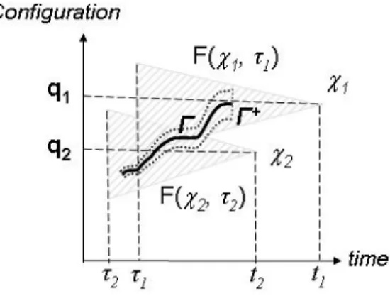
FIGURE 9: The geometry of CT-region F(χ, τk) for the 2D rod robot. 32 FIGURE 10: Predicted CT-space vs. Perceived CT-Space 36 FIGURE 11: The CT-regions contain the tunnel Γ+, which encloses Γ. 41
FIGURE 12: Illustration of the condition (24). 44
FIGURE 13: A situation after f(t) is shifted ∆t to end at t1. 44
FIGURE 14: Illustration of τe for CT-point χj. 48
FIGURE 15: Piece-wise continuous trajectory Γ consisting of three segments. 48 FIGURE 16: Piece-wise continuous trajectory Γ with two segments. 49 FIGURE 17: Snapshots of robot moving along a trajectory Γ. 53 FIGURE 18: Sensor data generated at a sensing moment. 55 FIGURE 19: An environment is viewed as a set of atomic obstacles. 56
FIGURE 20: Red circles as atomic obstacle. 58
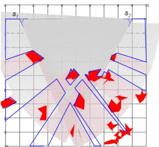
x FIGURE 22: Some free-space is represented as a part of atomic obstacles. 60 FIGURE 23: The union of free space visible from two sensors s1 and s2. 61
FIGURE 24: Ray intersection tests to detect an internal super pixel. 65
FIGURE 25: Neighborhood expansion of super pixels. 66
FIGURE 26: Illustration of some notations. 67
FIGURE 27: Division of a super pixel into smaller super pixels. 69
FIGURE 28: Illustrations of two cases of face RF 70
FIGURE 29: CFPA only considers a subset of atomic obstacles. 73
FIGURE 30: A 7-DOF Cyton arm. 75
FIGURE 31: Dimension of atomic obstacles for resolution 752 ×480. 75
FIGURE 32: Experiment and result. 76
FIGURE 33: An experimental environment with the stereo-vision sensor. 87 FIGURE 34: Snapshots of experiment #1 with a blue obstacle. 88 FIGURE 35: Snapshots of experiment #3 with a soccer ball as an obstacle. 89 FIGURE 36: Snapshots of experiment #5 with a plastic cover as an obstacle. 90
FIGURE 37: Simulation environment 96
FIGURE 38: Snapshots of an example run in simulation for vmax = 1 unit/s. 97 FIGURE 39: Effects of over-estimating vmax as vmax0 =cvmax,c≥1. 98
FIGURE 40: An example of static narrow passage. 99
FIGURE 41: A planar continuum manipulator. 100
FIGURE 42: Experiment with continuum manipulator in static environment. 101 FIGURE 43: Experiment with continuum manipulator (task 1). 102
FIGURE 44: Experiment with continuum manipulator (task 2). 103 FIGURE 45: Experimental setup for Robix Rascal RC 6. 105 FIGURE 46: An environment (Env1) and two traveled paths by the robot. 106 FIGURE 47: Selected steps taken by the robot in Env2. 106
FIGURE 48: A 7-DOF Cyton arm. 108
FIGURE 49: Dimension of atomic obstacles for resolution 188 ×120. 108 FIGURE 50: Snapshots of experiment #1 with vmax = 1cm/s. 110 FIGURE 51: Snapshots of experiment #2 with vmax = 3cm/s. 110
CHAPTER 1: INTRODUCTION
One of the ultimate goals in robotics is to enable robots to work autonomously in real-world environments. Meeting this goal requires the robot to move intelligently in environments without colliding with any obstacles, such as, chairs, tables, people, etc. Environments can be classified as follows:
• Static environment: No obstacles can move in the environment.
• Dynamic environment: Some or all obstacles can move in the environment. This dissertation introduces approaches for detectingguaranteedcollision-free robot motions in dynamic environments with obstacle geometries and their future motions unknown. This enables the robot to move autonomously and safely in such environ-ments. Finding such intelligent motions for a robot in an environment with obstacles is the task of a planner, which has been a central theme of robotics research. In the following, basic concepts about robots and environments are first introduced, and then the classical planners are surveyed.
1.1 Basic tool: C-Space and CT-Space
Planning can be defined by introducing Configuration Space (C-space) for a static environment, and Configuration-Time space (CT-Space) for a dynamic environment.
1. Configuration: A vector of independent variables q that defines uniquely the position of every point of a robot in a real world environment orphysical space. Figure 1 shows a robot arm with two joints expressed by vector [q1, q2]T in two
different configurations.
(a) (b)
Figure 1: A planar rod robot with two links and two joint variables [q1, q2]T.
2. Degrees of freedom (DOF): The number of independent variables that uniquely define the configuration of the robot. For example (Figure 2), a mobile robot has 2 to 4 DOF, an industrial manipulator has 5 to 9 DOF, a humanoid has 29 DOF, etc.
(a) Mobile robot with 3 DOF.
(b) Puma manipulator with 5 DOF.
3 Theconfiguration space(C-space) [62] of a robot has dimensions equal to degrees of freedom of the robot. The complex volume occupied by a robot at a configuration in physical space is represented as a point in the C-space [88]. Each point in the C-space is classified either as aC-obstaclepoint if an obstacle intersects with the robot at that configuration or as a C-free point, otherwise.
If obstacle poses i.e., their positions or orientations, change with time then the C-space also changes with time, i.e., a C-point which was a C-obstacle point may now become a C-free point and vice-versa. Planning in such a space, which changes when an obstacle moves, is difficult. Thus, the notion of configuration-time space (CT-space) is introduced by adding one more dimension of time to the configuration space; each CT-slice at a time instant of a CT-space corresponds to a C-space at that time instant. A CT-point χ = (q, t) corresponds to a robot at a particular configuration q at a particular time t in the physical space. The C-obstacles on all the CT-slices define CT-obstacles in the CT-space, and the remaining space is the CT-free space. Figure 3 shows an example of CT-space of a 2 DOF robot and a collision-free motion segment (trajectory) that connects the starting configuration S
to the ending configuration G.
The notions of paths and trajectories for robot motion are defined below:
• Path: A 1D curve segment in the C-space of the robot representing the sequence of configurations of the robot.
• Trajectory: A 1D curve segment in the CT-space of the robot representing the sequence of poses that the robot will be at different time.
Figure 3: CT-space of a 2 DOF robot
A planner tries to find a sequence of motions for the robot to reach the goal con-figuration from the start or the current configuration, without colliding with any obstacles. This sequence of motions is a (a) collision-free path in the C-free space of the robot, if the environment is static, or (b) collision-free trajectory in the CT-free space of the robot, if the environment is dynamic. Figure 3 shows a collision-free trajectory (motion segment) in the CT-space of the robot that connects the starting configuration S at timet = 0 to the ending configuration Gat time t=tG.
1.2 Different kinds of real-world environments
Robots, working in a real-world environment, must have complete or partial infor-mation about obstacles or available free-space in that environment. Depending on whether an environment is static or dynamic and the level of information available to the robot, environments can be classified into different categories.
1.2.1 Known environment
A known environment is usually man-made, where the information about it is completelyknown. Such an environment can be static or dynamic as discussed below:
5 • Static environment: In a man-made static environment, precise geometries of obstacles can be known. For example, industrial environments, such as, a man-ufacturing site, consists of obstacles, such as, machines, parts, etc. with their geometric models usually known. Thus, most required information about the physical environment for robot motion planning is available.
• Dynamic environment: In a known dynamic environment, future motions of ob-stacles are precisely known along-with their geometries. For example, multiple robots working in the same environment can consider other robots as obsta-cles with known motions. Such a kind of environment is commonly found in industrial environments, where robots try to manipulate some objects in the environment. Thus, most information about environment for planning is avail-able.
1.2.2 Unknown static environment
An unknown static environment is where objects are unknown but nothing moves, such as some ancient ruins or the surface of Mars. In such an environment, models of obstacles are not known, which further complicates detection of obstacles as particular objects in real-world. Thus, the required information about environment for planning robot motion has to be gained from sensing.
1.2.3 Partially unknown dynamic environment
A partially unknown dynamic environment contains obstacles, whose geometries are known but their motions are unknown. Moreover, obstacles are often constrained to move only within a specific region due to the nature of environment or behaviors of
obstacles themselves. For example, on highways, where the roads are clearly divided by lanes, vehicles can move along only one side of the road and possibly within their lanes for some time period; also, the geometries of vehicles are known as they are manufactured by various vehicle manufacturers.
Since the possible obstacle motions could be known based on the constraints on their motions, their future motions can be predicted by tracking their past motions. Sensing is required to detect obstacles for planning robot motion in such an environ-ment.
1.2.4 Unknown and unpredictable environment
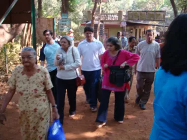
An unknown and unpredictable environment is where obstacles are completely unknown and their motions are unknown or hard to predict. For example, people moving in shopping malls or offices or at home. Moreover, in such environments, not all possible obstacles that a robot is likely to encounter can be known. Figure 4 shows an example. Since possible future obstacle motions are difficult to know, their future
7 motions can be wrongly predicted. Thus, the information about an environment, obtained through obstacle recognition and motion prediction, may not work here. New ways are called upon to acquire information.
1.3 Planning robot motion
Planners in the robotics literature can be categorized based on the kinds of envi-ronments in which robot motions are planned and are described here.
1.3.1 Path planning
If the environment is static, a planner needs to find a path, connecting the start pose of the robot to the end pose, in the C-free space of the robot. Such kind of planning is called path planning. The primary focus of the planner is not only to find the existence of a collision-free path, but also to find the best path depending on optimization parameters. For finding the existence of a collision-free path there are approaches for 2D or 3D C-space that use C-obstacle features, such as, vertices of polygonal C-obstacles [63], edges of polygonal C-obstacles [47], etc. If C-obstacle geometries are not known, then approximate cell-decomposition [53] is used to com-pute the approximate geometry of C-free space in the C-space. The commonly used optimization parameters are shortest path, minimal robot energy, minimal time, etc. Computing C-obstacles is not only difficult [34,93], but also infeasible if the C-space is high dimensional for a robot with high-DOF, such as, manipulators, humanoids, etc. Sampling based approaches [46,55,56] have been used extensively to avoid computing C-obstacles. These approaches randomly find a set of collision-free C-points (nodes) and then locally try to find collision-free paths that connect the nearby nodes. The
randomness in picking nodes is primarily used to ensure good coverage of C-space. Testing if a C-point is a part of any C-obstacle just requires collision-checking, which is described later in the next section. However, such planners may not be able to find a solution if one exists; increasing sampling of C-points increases the probability of finding a solution and thus, such planners are probabilistically complete. One representative planner is the probabilistic roadmap method [46] and there exists a well-studied literature on sampling schemes [2, 59, 71] for representing free-space in the C-space of a robot.
1.3.2 Reactive planning
In certain environments, only some obstacles may be dynamic among other static obstacles. Then, planning can be done in the robot’s C-space as described in the above section; for some dynamic obstacles, a found collision-free path among static obstacles can be modified locally as the robot starts executing that path [45, 103]. Such local planning, where the planner just locally reacts to the obstacles is known as reactive planning. Reactive planning is computationally less expensive than path planning or motion planning (described in next section) that uses global information about an environment, i.e., account for the presence of all the obstacles. Thus, a reactive planner can easily generate a local plan in real-time; however, it cannot direct the robot to reach the goal without the help of a path planner and can often get the robot stuck in local minima.
9 1.3.3 Motion planning
If an environment is dynamic, a planner needs to find a trajectory connecting the starting configuration-time to the ending configuration-time in the CT-free space of the robot, and that is called motion planning.
If the future motion of an obstacle is known for a long time period, then a CT-obstacle corresponds the swept volume over time of a C-CT-obstacle. The approaches [47, 63] mentioned in section 1.3.1 can be used when C-obstacles can be computed. How-ever, finding the swept volume of a complex obstacle is difficult. Moreover, computing C-obstacles becomes difficult or even infeasible as the DOF of robot increases. Similar to path planning, sampling-based approaches [46, 55] could be used here except that the planning is done in the CT-space of the robot.
If the future motions of obstacles are not known beforehand, then it can be es-timated or predicted so that the planner is able to find a solution from starting configuration to ending configuration. In general, the estimation or prediction of fu-ture motions of obstacles are usually true only for a short period immediate after the time when the prediction is made. This causes the estimated CT-space of the robot to keep on changing over time as obstacles behave differently from their predicted behaviors. This makes planning more difficult as a detected collision-free trajectory may not really be collision-free. A common approach is to re-plan those parts of trajectories that now lie on CT-obstacles (e.g., [92, 108]).
1.4 Collision-checking
Computing C-obstacles or CT-obstacles is difficult and can be infeasible if the com-plexity of physical obstacle geometry or the DOF of the robot is high. As discussed in section 1.3.1, sampling based planners could be used here as they only require to know if a C-point/CT-points in C-space/CT-space is collision-free or not. The following two common approaches, depending on whether the obstacle geometry is known or not, can easily compute such information in 3D physical space of the robot: • Model based checking: When the 3D obstacle geometry is known, the obsta-cle can be modeled using (a) simple bounding volumes such as object oriented bounding boxes (OBBs), spheres, capsules, etc, or (b) a set of polygonal faces (called mesh) such as triangles, rectangles, etc. Figure 5 shows an example. There exist well-studied literature [15, 61] in the field of computer graphics that can efficiently detect the existence of intersection between simple bounding vol-umes or meshes. For example, the separation axis method uses convex property of polyhedral objects to determine quickly if an intersection exists or not be-tween them. For intersection checking bebe-tween meshes, hierarchal checking is often used, where a complex mesh is represented by simple bounding volumes. • Occupancy in physical space: If the obstacle geometry is not known then the
physical space can be divided into voxels, which are small cubes; and whether the voxel is obstacle free or not can be determined by sensing (e.g. [104]). A robot at a particular configuration occupies a set of voxels in the physical space, which can be determined as the geometry of robot is known. One approach [58]
11
(a) Bounding box roughly approximates the obsta-cle.
(b) Mesh closely approxi-mates the obstacle (Stan-ford bunny).
Figure 5: Approximating real obstacle geometry.
computes off-line the mapping between a set of C-points and its corresponding set of voxels in the physical space. Although such collision-checking may be faster than the model based checking, it restrains the planner to use only those C-points for which mapping has been computed.
As this dissertation is focused on tackling the largely open problem of how to detect collision-free robot trajectories in unknown and unpredictable environments, it is important to first examine existing approaches related to detecting collision-free robot trajectories. These approaches often assume that much information about an environment is known. Related literature includes methods for continuous collision checking, approaches for acquiring information of an environment through sensing, and approaches in control focusing on handling robot motion uncertainty.
2.1 Assumptions made about dynamic environments for robot motion Geometries of obstacles and their future motions are known: As the geometry, pose, and motion of any obstacle is completely known, planning can be done off-line using a model of the environment without the need of sensing. Sensing is used only during actual execution of a robot’s motion to deal with uncertainties (e.g., [51,72,84]). Some approaches are focused on finding collision-free regions or free space in the C-space [53, 98]. If the robot has high degrees of freedom (DOF), such as, an articulated robot, the corresponding C-space and CT-space are high-dimensional. To avoid construction of high-dimensional C-obstacles (or CT-obstacles), sampling-based planners are widely used [46, 55].
inter-13 val can be computed: Here one common focus is on-line revising pre-planned paths in previously known environments to avoid robot collisions with newly added recog-nizable obstacles, which could be static (e.g., [58]) or performing particular kinds of motions (e.g., [103, 108]). These schemes usually assume partial changes to known C-space or CT-space to limit the scale of re-computing or re-planning for facilitating real-time computation. There is also work on motion planning to avoid static or moving obstacles with certain known velocities within some time interval [25, 52]. Only the geometries of obstacles are known: Here the obstacles are assumed known (or recognizable), but with unknown future trajectories. There are a few planners (e.g., [20, 35, 50, 89]) that address mobile-robot motion planning in such an environment. A real-time adaptive motion planning (RAMP) approach [91, 92] is very effective for planning high-DOF robot motion, characterized by simultaneous planning and execution based on sensing.
Most approaches commonly predict future obstacle trajectories by tracking the past motions of the known obstacles (e.g. [12, 21–23, 27, 32, 36]). However, the predic-tion is usually true only for a short period, i.e., immediately after the time when the prediction is made. As the observed behavior of an obstacle changes, the prediction of the obstacle’s future trajectory changes. Thus, planning future robot’s motion is based on frequently updating the predictions, and unknown changes in an environ-ment are taken into account by repeated computations or re-computations of (some parts of) paths/trajectories, which involve repeated collision checking. Moreover, the planned motions may also fail to be collision-free due to inaccurately predicted obsta-cle motions. There exists work aimed at guaranteeing collision-free motions for mobile
robots. The notion of “Inevitable Collision Regions” (ICS) was introduced [28] for a mobile robot to characterize guaranteed CT-obstacles in its CT-space. Further, there has also been some approaches introduced in [29] that guarantee motion safety of a robot by assuming specific conditions, such as, the robot observes unicycle dynamics, obstacles are also robots, etc.
Geometries of obstacles are known and all possible motions of obstacles are taken into account: In [90], prediction of unknown motions of known obstacles is avoided by considering all the possible future motions of the obstacles, i.e., considering worst-case CT-obstacles so that the planned motions are guaranteed collision-free. However, the estimated free CT space is too conservative (i.e., too small due to exaggerated CT-obstacle regions) and increasingly so with time, as possible poses of obstacles increase with time. Also, in [101], the precise reachable motions of circular disc obstacles, observing unicycle dynamics, are computed to guarantee safety for infinite time horizon.
2.2 Extracting information from sensing in unknown environments
Planning requires to know information about environment, such as, geometries of obstacles and their future motions. If obstacle geometries and their motions are unknown, then sensor(s) can be used by the robot to gain information about the environment. However, the kind of sensor data generated by real sensors are very rudimentary and do not directly provide high-level information of object models. There exists a vast literature that addresses this problem of inferring information about an environment from sensor data and are discussed in this section.
15 2.2.1 Acquiring information of obstacles
Any moment, the planner needs to know the current pose occupied by the obstacles or the available free space. For dynamic environments, the planner additionally needs to know how the obstacles poses change with time or the way the available free-space changes with time. There are mainly two approaches that try to infer information about the occupancy of obstacles in an environment:
Finding obstacles: From sensor data, if an obstacle in the environment can be identi-fied using its features, then based on poses of features along with the known geometry of obstacles, the occupancy of that obstacle in the physical space can be obtained. Two most common approaches for 3D modeling are (a) 3D modeling tool used while designing that object (obstacle), and (b) scanning real-world object using different kind of sensors (e.g. [24,38]), such as, laser scanner, stereo-vision, camera, etc. How-ever, identifying obstacles from sensor data itself is an active research area as each obstacle has different kind of features and complexities. For example, in computer vision, a major focus of research is to identify specific kinds of objects, such as, hu-man [4, 33], vegetation [7], objects that can cause a mobile robot to drop off [69], internal organs or parts in human bodies for medical analysis [44], etc. There exist common methods [73, 79, 100], especially from machine learning [48, 107], that can be used to detect various kinds of objects. Such methods often require time consuming training process, but the training could be done off-line and a mapping function, which identifies a specific object or object class from other objects, determined as a result of training, could identify that object instantaneously. The major issue with
such approaches is the lack of guarantee to have high accuracy for identifying an object due to many factors, such as different lighting conditions, occlusions, etc. Finding free physical space: There is much research on how to represent and sense an unknown (mostly static) environment using robots with sensors mounted. One approach represents an unknown static environment with unknown obstacle geometry in terms of voxels [104]. However, detecting all voxels occupied by the actual obstacles from sensing is not a trivial matter and may not be feasible in real-time. A large body of work is focused on simultaneous robot localization and mapping (SLAM) in an unknown static environment [86], which represents the environment using probability distributions.
There is also research addressing how to move a robot to maximize sensing views (i.e., minimize occlusions) [106]. For sensor-based robot navigation, different kinds of sensors are used, either mounted in the environment to provide a world view, or mounted on a robot to provide a robot-centric local view. The planners, referred to as sensor based motion planners [31, 105], are often adapted from classical model based planners to plan paths incrementally, as the unknown static environment becomes known gradually from sensing. However, for unknown dynamic environments with obstacle geometries not known, planning becomes difficult.
2.2.2 Future changes in an environment
For planning robot motion in a changing environment, the future information about that environment must be known. The future change in the environment can be estimated if the change in obstacle poses can be estimated, or dually the change in
17 available free-space in physical space can be estimated.
Predicting future obstacle motion based on its past motion or its current motion has been widely used in literature. The common motion model performed by any obstacle is well defined in the literature of Physics, such as Newton’s law of motion, Newtonian dynamics, Lagrangian mechanics, etc. The kind of predictions commonly made in literature for planning robot motion are described below:
Short-term prediction: If the prediction is made based on only the current state of the obstacle, then the prediction about obstacle motion is accurate as long as the obstacle is not obstructed or the obstacle, itself, decides to change its motion. As no past information is known, the event of such occurrence, i.e., obstacle changing its motion, can not be known based on the current state of the obstacle. Thus, predictions are true usually for a short period of time. Such a kind of prediction [12, 70] is widely used for reactive planning [25, 52] (see Section 1.3.2).
Long-term prediction: Using the past information of an obstacle may enable predict-ing for longer period. One approach [27] considers uspredict-ing the notion that obstacles move in a way so as to achieve their point of interest. Other approaches [5, 13, 21, 91] try to find some repetitive pattern occurring by tracking obstacle motion all the time, for long-term prediction. Since, the precise future obstacle motion may not be known, multiple possible future trajectories [67] for each obstacles need to be considered for planning, which can increase collision-checking cost. Moreover, identifying a single obstacle in a complex environment itself is difficult as discussed in Section 2.2.1. Thus, tracking multiple obstacles [12, 21–23, 27, 32, 36] is not only difficult but the compu-tational complexity grows as the number of obstacles increases in an environment.
2.3 Collision detection
Collision detection is usually the most time consuming component of any sampling-based robot motion planner. Many fast collision-checking algorithms [15, 42, 61] exist for detecting collisions between two arbitrary stationary objects represented by polygonal meshes or sphere trees. Recently, an efficient collision detection algorithm [60] is introduced for checking collisions between the exact model of a continuum manipulator and obstacles in polygonal meshes.
Checking for collisions of a robot path or trajectory is usually done by discretizing the path/trajectory and check for each discretized configuration, which may omit col-lisions with small obstacles, depending on the resolution of discretization. Therefore, there also exists some work that addresses continuous collision checking of a robot path/trajectory. Most of such work requires known obstacle motions. One approach formulates trajectories of the robot and approximated obstacles in the environment as functions of time and finds the time instants when collision occurs analytically [81]. However, if the trajectory functions are nonlinear, solving for collision time instants can be difficult. The adaptive bisection algorithm [80] is based on the intuition that if the sum of the distances traveled by two objects is less than the minimum distance between them before traveling, then they cannot collide during their motions.
There are also approaches in the literature that focus on generating or approximat-ing the continuous swept volume by a robot along a path or trajectory [11, 26], which can then be used to perform collision tests against obstacles. One approach [76] mod-els the motion between two discrete configurations of an articulated robot in order
19 to avoid generating the swept volume of individual links. Graphics hardware is then used to perform fast collision queries for approximated swept volumes in a virtual prototyping environment. Another approach [3] is focused on growing the physical robot’s volume at discrete configurations along a path to form a continuous region for collision tests. These approaches are focused on the moving robot rather than the obstacles, which are mostly assumed static.
2.4 Handling motion uncertainty of robot in planning
Uncertainty in robot configuration while planning robot motion is well studied in the literature. Different kind of uncertainties resulting from different factors, such as stabilizing a non-holonomic system [9], slipping of wheels [19], etc. has been studied for a mobile robot. Further in [99], it has been shown by deriving equations specific to that robot, uncertainty in robot control can be easily handled. Such approaches are focused more on reducing uncertainty for specific robots than considering collision avoidance with obstacles.
The approach [77] relies on known environment features (map) to handle uncer-tainty in robot configuration; also, there exists approaches (e.g., [66]) to deal with uncertainity in a map. If the environment is unknown and static, there exists a body of literature [41,86] that simultaneously handles uncertainty in robot localization and mapping of an environment.
Some researchers addressed uncertainties in motion planning algorithm, e.g., [49, 54, 72]. The approach [30] introduces the notion of a robust path that guarantees a non-holonomic mobile robot to reach its goal based on landmarks.
2.5 Limitations
The following limitations hold for the existing methods in detecting collision-free robot trajectories in an uncertain, dynamic environment:
• The approaches based on predicting known obstacle motions may be too expen-sive due to the non-trivial process of obstacle identification and the repeated computations of their predicted motions, especially if there are many obstacles, which leads to repeated collision checking for detecting collision-free robot tra-jectories, which can be infeasible in real-time for high degrees-of-freedom (DOF) robots.
• The planned robot motions may fail to be collision-free, i.e., unsafe, if future obstacle motions are predicted inaccurately.
• Planning in an environment that is unknown and unpredictable, i.e., obstacle geometries are unknown and their future motions can not be predicted, is more challenging, and to the best of the author’s knowledge, no current approach can tackle that.
These limitations motivate the proposed research and shed light on the value of contributions of this dissertation.
CHAPTER 3: RESEARCH OUTLINE
One of the fundamental abilities required by motion planners is to test if a motion performed by a robot will collide with any obstacles or not. The focus of the disserta-tion is to present novel approaches/algorithms that enable a modisserta-tion planner to know if a future motion of the robot is collision-free or not based on sensing in an unknown and unpredictable environment.
3.1 About unknown and unpredictable environments
In an unknown and unpredictable environment all or some obstacles can move in any direction. Moreover, objects can appear or disappear from a real-world environ-ment, become separate into smaller objects or combine into bigger ones, for example, in human centered environments, such as domestic environments, office environments, etc. Even for environments well known to humans, the number and variety of obsta-cles can be practically uncountable and not constant.
A robot operating in such an environment neither knows the possible kinds of obstacles (i.e. their geometries) nor the kinds of motions they could perform. How to enable a robot to move safely in this kind of environments is an open challenge.
3.2 Online determination of collision-free CT-points via sensing
A robot needs to actively sense to acquire information about its unknown envi-ronment. A sensor can sense only a part of a physical space, where the robot goal
configuration may not be visible. Many sensors could be used to sense the physical space, however, the amount of sensor data generated could be huge, which could make it difficult for planners to find collision-free motions in real-time.
The rate at which the information about the environment is gained, determines whether a planner can plan robot motions in real-time. Many sensors generate sensor data at the rate of 20Hz-80Hz. Within a sensing cycle, the planner must be able to detect multiple collision-free CT-points for decision making in real-time. Thus, how to quickly determine collision-free CT-points from sensor data is a major challenge, especially for high degree-of-freedom robots.
3.3 Detecting safe trajectories for a robot
For a robot to operate in a real-world environment, especially one involving humans, the robot must not hit any obstacles. While a simple solution is to make the robot stop its motion, it can get damaged by a moving obstacle. If a robot is set to execute a trajectory, the trajectory should not be merely collision-free, rather, it is better guaranteed collision-free in spite of unknown motions of obstacles.
Further, all the possible configurations that can be reached by the robot, which cannot execute a trajectory precisely, need to be guaranteed collision-free. This can be modeled as a certain “tunnel” of collision-free trajectories, which needs to be detected ascontinuouslycollision-free, i.e., every CT-point in that tunnel is collision-free. How to enable fast detection of a tunnel of guaranteed collision-free trajectories is a novel challenge that has not been addressed.
23 3.4 Outline
Our research contribution is to introduce approaches that, (a) do not require iden-tifying individual obstacles, (b) do not require tracking to predict obstacle future motions, and (c) do not consider all possible motions of all obstacles for infinite time horizon but rather use progressive sensing to perceive collision-free high-DOF robot trajectories in real-time. Moreover, the detected trajectories will be guaranteed con-tinuously collision-free and safe in spite of robot motion uncertainty.
The rest of the dissertation is outlined below. Chapter 4 introduces the notion of dynamic envelope for detecting a collision-free CT-region associated with a CT-point
χ = (q, t), under an assumption that the obstacle speeds range in [0, vmax]. As the robot cannot execute a trajectory Γ precisely, we assume that it will move within some continuous tunnel Γ+, which describes motion uncertainty when the robot executes trajectory Γ. An algorithm is introduced in Chapter 5 to detect Γ+ as
collision-free using only a finite set of CT-points Q(Γ+), which when discovered guaranteed
collision-free, implies that Γ+ is guaranteed collision-free.
Chapter 6 introduces the notion of atomic obstacles to characterize the obstacles directly from sensor data for any sensing moment. The concept of atomic obstacles avoids identifying obstacles, considering that not all obstacles need to be identified and obstacle identification and tracking are often difficult or expensive to do. Chapter 7 introduces a fast real-time collision detection algorithm between a high DOF robot and a large number of atomic obstacles.
atomic obstacles, introduced in Chapter 5, to detect collision-free CT-points via a general online sensor-based algorithm called Collision Free Perceiver using Atomic obstacles (CFPA). Next, we focus our attention in embedding CFPA into a real-time motion planner, taking into account the finite processing time that CFPA requires, in Chapter 9. Chapter 10 demonstrates experiments and results for the approaches. Chapter 11 concludes the dissertation and discusses directions for future work.
CHAPTER 4: DYNAMIC ENVELOPE
One of the important factors that facilitates real-time motion planning of high-DOF robots is the ease of knowing if the robot can stay safely at a configuration q for given future time t. Dynamic envelope is a novel concept that allows a robot to know if a configuration-time point (CT-point) χ= (q, t) is guaranteed collision-free or not, without knowing future motions of obstacles. Further, it can also be used to detect a collision-free continuous CT-region that is in a neighborhood of CT-pointχ. For some future time t, dynamic envelope is defined based on the robot model, vmax assumption about the environment, and a sensing momentτ.
4.1 Robot model
We assume that a high-DOF robot consists of multiple polyhedral links. This is a reasonable assumption since a real robot’s link is commonly modeled by a polygonal mesh, or can be approximated by a polyhedral bounding box.
The following notations describe such a robot model in the Cartesian space R3 (physical space).
• l: the set of points constituting a polyhedral link (rigid body) of the robot. • lx: the set of vertices of l.
R(q) =S
l(q).
• Rx(q): the set of all bounding vertices of all links of the robot at configuration q, i.e. Rx(q) =
S
lx(q).
• p(q): the position of a pointp∈R in the Cartesian space when the robot is at configuration q.
• px(q): the position of a point px ∈Rx in the Cartesian space, when the robot is at configurationq.
4.2 vmax assumption about the environment
For an unpredictable environment, we assume an upper bound on the maximum possible linear speed vmax of any obstacle. The value of vmax can be obtained for different real world environments. For example, in a city environment where people and cars move, vmax can be determined based on the speed limit on a vehicle, and in a pedestrian only area,vmax can be set as the maximum walking/running speed of a person. Any obstacle may have varied actual speeds in [0, vmax]
4.3 Sensing instant τ
At every sensing moment τk, k > 0 the sensor generates new rudimentary sensor data. For motion planning, within a sensing cycle [τk−1, τk] the information about the poses of obstacles in the environment need to computed from the sensor data. We use the following notation to indicate obstacles sensed at time τ in the robot’s physical space:
27 4.4 Definition and its properties
Definition 1: For a robot’s configuration-time (CT) point χ = (q, t), a dynamic envelope E(χ, τ), as a function of current sensing time τ ≤ t, is a closed surface enclosing the region R(q) occupied by the robot at configuration q in the physical space R3 (or
R2 for 2-D planar space) so that the minimum distance between any
point on E(χ, τ) and the regionR(q) is
d(t, τ) =vmax(t−τ) (1)
Theorem 1: For a CT-point χ= (q, t), if E(χ, τ)∩O(τ) =∅ at sensing time τ < t, then χ is detected as guaranteed collision-free, i.e., no obstacle will hit the robot at
χ no matter how obstacles move. Proof:
Since vmax is the upperbound of all actual obstacle speeds at any time,E(χ, τ) has the following general properties:
1. It shrinks monotonically over sensing time with speed vmax, i.e., E(χ, τk+1) ⊂
E(χ, τk), where i >0,τk < τk+1 ≤t. E(χ, τ) shrinks to R(q) at t.
2. An obstacle not on or inside E(χ, τk) will never be on or inside E(χ, τk+1).
3. An obstacle either on or inside E(χ, τk) can be outside E(χ, τl) for some τl ∈ (τk, t], if not moving towards R(q) in maximum speedvmax.
Hence, at any timeτk, if no obstacle is on or inside the dynamic envelopeE(χ, τk), i.e.,
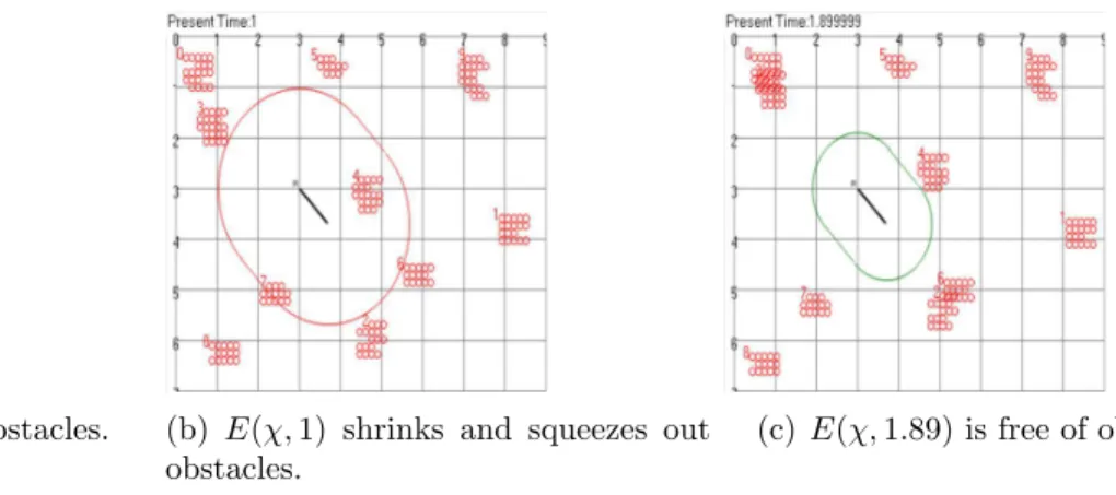
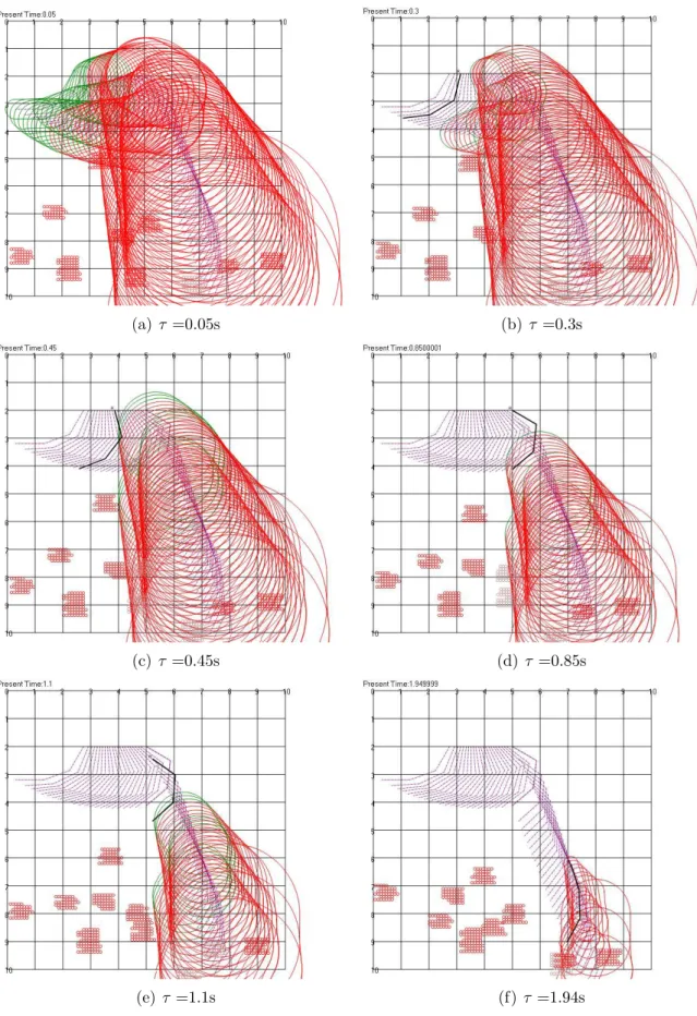
(a) E(χ,0.1) contains obstacles. (b) E(χ,1) shrinks and squeezes out obstacles.
(c) E(χ,1.89) is free of obstacles.
Figure 6: A dynamic envelope of a planar rod robot. and χ is guaranteed collision-free.
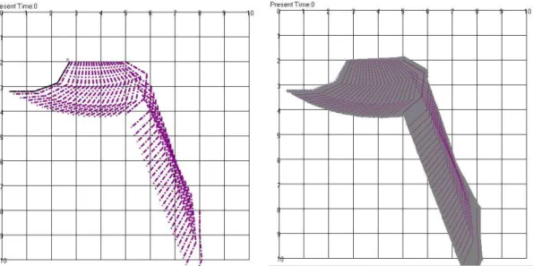
Figure 6(a) shows an example of a dynamic envelope for a planar rod robot in 2-D environment, where χ = ((3,3),3), τi =0.1s and vmax = 1 unit/s. At τ = 1.89s, χ is detected guaranteed collision free.
As soon as a dynamic envelope E(χ, τ) is free of obstacles at a sensing instant τl, it has achieved the purpose of detecting that χ is collision-free. Thus it is no longer needed and canexpireatτl. If a dynamic envelope is first used at timeτ0 and expires
later atτl, we call [τ0, τl] its life span.
As R(q)⊂E(χ, τl), more neighboring CT-points are discovered collision-free: • Time-wise: Since no obstacle can be inside dynamic envelope within time
inter-val [τl, t], all the continuous configuration-time points within that time interval for configuration q are guaranteed collision-free.
• Space-wise: For other neighboring configuration q0, we could find a dynamic envelope E(χ0, τl), such that E(χ0, τl) ⊂ E(χ, τl) (see Figure 8), where χ0 = (q0, t0), then χ0 is also guaranteed collision-free. Finding such CT-points are
29
Figure 7: Illustration of dmax(q0,q) of a rod robot. shown in the next section.
4.5 Collision-free CT-region discovered along with a CT-point
As a dynamic envelope of a CT-point always contains R(q), it is interesting to find an another configuration q0, so that the dynamic envelope of that CT-pointχ= (q, t) contains R(q0) within certain lifespan of the dynamic envelope. The distance
dmax(q0,q), defined as,
dmax(q0,q) = max ∀px∈Rx
kpx(q0)−px(q)k. (2)
is useful for this purpose. Figure 7 illustrates dmax(q0,q) of a rod robot (which can also be considered a rectangular link of a high-DOF robot).
We have the following theorem.
Theorem 2: When a CT-pointχ= (q, t) is discovered collision-free at a sensing time
τl, i.e., the dynamic envelope E(χ, τl) is free of obstacles, a continuous neighborhood
F(χ, τl) ofχis also discovered collision-free, such that, for any CT-pointχ0 = (q0, t0)∈
F(χ, τl), its configurationq0 satisfies:
Figure 8: Illustration of inequality (5). and its time t0 satisfies
τl ≤t0 ≤t−
dmax(q0,q)
vmax
< t. (4)
Proof: When inequality (3) is satisfied, R(q0) is contained by the dynamic enve-lope E(χ, τl), which is free of obstacles. If χ0 = (q0, t0) is collision-free, it means that the dynamic envelope of χ0 is contained in the dynamic envelope of χ, i.e.,
E(χ0, τl)⊂ E(χ, τl), and τl ≤t0. Since dmax(q0,q) is the maximum distance between two corresponding points of R(q0) and R(q), we have
dmax(q0,q) +vmax(t0−τl)≤vmax(t−τl), (5)
which can be simplified to
t0 ≤t− dmax(q 0,q)
vmax
.
Thus, the theorem is proven.
Figure 8 illustrates the proof for a rod robot.
Corollary 1: Ifχ0 ∈F(χ, τl) for someτl < t, thenχ0 ∈F(χ, τl+m), τl+m ∈[τl, t0], m≥ 0
31 Proof: From inequality (4), subtracting t0, we have
0≤(t−t0)− dmax(q 0,q)
vmax which, multiplying vmax, leads to:
dmax(q0,q)≤vmax(t−t0)
From the above, because τl+m ≤t0, we have
dmax(q0,q)≤vmax(t−τl+m) (6) and also τl+m ≤t0 ≤t− dmax(q0,q) vmax < t. (7)
With (6) and (7), based on Theorem 2, the corollary holds.
We next characterize the geometry of the CT-region F(χ, τl) below, based on The-orem 2 and Corollary 1.
• F(χ, τl) is on the time interval [τl, t].
• The region of F(χ, τl) on the time-slice τl contains all the configurations that satisfy inequality (3), whose size and shape depend on (a) the robot kinematics, and (b) the size of the dynamic envelope E(χ, τl).
• At the time-slice t, F(χ, τl) contains the single CT-pointχ= (q, t). • Based on Theorem 2, forτl ≤t0 ≤t(χ,q0), where
t(χ,q0) = t− dmax(q 0,q)
vmax
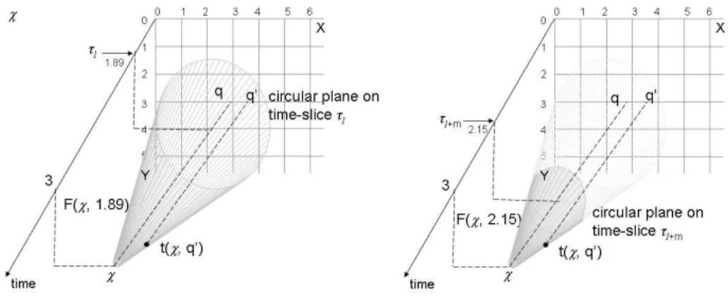
(a) F(χ,1.89) based on the dynamic enve-lopeE(χ,1.89) shown in Figure 6(c).
(b)F(χ,2.15) based on the dynamic enve-lopeE(χ,2.15). F(χ,2.15)⊂F(χ,1.89).
Figure 9: The geometry of CT-regionF(χ, τk) for the 2D rod robot.
all CT-points χ0 = (q0, t0) are in F(χ, τl). Equation (8) shows that the smaller
dmax(q0,q) is, the longer is the hyper-line from (q0, τl) to (q0, t(χ,q0)) inF(χ, τl). • dmax(q0,q) decreases with slopevmaxast(χ,q0) increases fromτltotas indicated
by the following equation derived from (8).
dmax(q0,q) = −vmaxt(χ,q0) +vmaxt (9)
• F(χ, τl+m) =F(χ, τl)−Fp, where Fp ={(q0, t0)|(q0, t0)∈F(χ, τl), t0 < τl+m}. As an example, Figure 9 illustrates the geometry of the CT-region F(χ, τl) of the same rod robot with no width as in Figure 6 with only two translational degrees of freedom. The region ofF(χ, τl) on the time slice τi is a circular disc.
Thus, a dynamic envelope not only discovers a collision-free CT-point but also its neighboring CT-region. Moreover, without assuming any future motions of obstacles, based on vmax assumption, the tool successfully discovers collision-free CT-points. Next, we show the effects of over exaggerated vmax assumption for our approach.
33 4.6 Robustness of approach over exaggeratedvmax
As vmax, the maximum speed of an obstacle, is the only known or estimated pa-rameter we assume in our approach dealing with an unpredictable environment, it is necessary to investigate how robust our approach of detecting collision-free CT-space points is ifvmax is over-estimated asvmax0 > vmax. The effect of such over-estimation can be stated in the following theorem.
Theorem 3: Let vmax0 = cvmax, c > 1, and let χ = (q, t) be a collision-free CT-point. Let E(χ, τ) and E0(χ, τ) be the dynamic envelopes defined by vmax and vmax0 respectively. If (q, t) is detected collision-free at τl by E(χ, τl), then, (q, t) will also be detected collision free byE0(χ, τl0), such thatτl < τl0 and τ
0
l =τl+ (c−c+p1)(t−τl)≤t, where −1≤p≤1.
Proof: Suppose at time τ0, we start observing the dynamic envelopes E(χ, τ0) and
E0(χ, τ0) with respect to vmax and v0max, where, based on equation (1),
d(t, τ0) = vmax(t−τ0), and
d0(t, τ0) =v0max(t−τ0) = cvmax(t−τ0)
Clearly for any timeτ0 ≤τ < t, E0(χ, τ) is larger thanE(χ, τ). Suppose further that
at least one obstacle was on or insideE(χ, τ0), then it was also on or inside E0(χ, τ0).
Suppose at time τl, where τ0 ≤ τl ≤ t, the dynamic envelope E(χ, τl) has shrunk enough to just “squeeze out” obstacles and detected that the CT-point (q, t) is collision-free. Let dmin(q, τl) denote the minimum distance between R(q) and the obstacles. Thus,
where > 0 is infinitesimally small. Clearly at τl, E0(χ, τl) still has an obstacle because it is larger than E(χ, τl).
However, according to Definition 1 and equation (1), d(t, t) = cvmax(t −t) = 0. Since (q, t) is a collision-free CT-point, it means that E0(χ, t) at sensing time t is free of obstacle. Since E0(χ, τ) shrinks continuously as τ progresses towards t, there exists a momentτl0,τl < τl0 ≤t, whenE
0(χ, τ0
l) is free of obstacle and (q, t) is detected collision-free.
We now see how τl0 is related toτ. Based on equation (1),
d0(t, τl0) =cvmax(t−τl0) =dmin(q, τl0)−. (11)
Since obstacles never move with speed greater thanvmax, fromτl toτl0, the change in minimum distance between R(q) and obstacles can be expressed as:
dmin(q, τl0)−dmin(q, τl) =pvmax(τl0−τl), −1≤p≤1. (12)
From the equations (10), (11), and (17), we have
d0(t, τl0)−d(t, τ) =pvmax(τl0−τl), −1≤p≤1 (13)
From (10), (11), and (13), we can further obtain
τl0−τl = (
c−1
c+p)(t−τl)≤t−τl (14)
Based on Theorem 3, τl0 =t corresponds to the worst case scenario where p=−1, meaning that the closest obstacle toR(q) atτoriginally insideE(χ, τ0) moves towards
35
R(q) with vmax fromτ tot, and in all other cases,τl0 < t.
The significance of the theorem is that, if a CT-point (q, t) is collision-free, then it will be detected as collision-free no later than timet no matter how badly the actual
vmax is overestimated as v0max. This shows the robustness of our approach. 4.7 Perceived CT-space
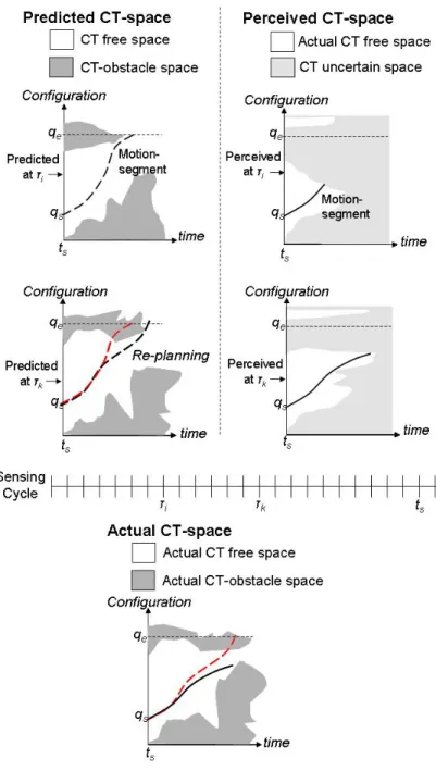
An important tool required for motion-planning of robot in a dynamic environment is the CT-space (see section 1.1) of the robot. In an unknown and unpredictable environment, as the motion of obstacles are unknown, a common way is to predict obstacles motion and the corresponding CT-space of the robot we call as Predicted CT-space; whereas, using our approach of dynamic envelope, which requires to know only poses of obstacles at a current sensing moment τ, the corresponding CT-space we call as Perceived CT-space.
The motion planner must plan the motion on true collision-free regions, or free space, in the CT-space of a robot. However, with the prediction mechanism, being true only for a short period of time, does not guarantee that the motions planned lie on true collision-free regions. Whereas, with dynamic envelopes true collision-free regions can be perceived. We illustrate this by an example.
Figure 10 compares predicted vs. perceived vs. actual CT-space in a 2-D example. Both predicted CT-space and perceived CT-space will change as sensing/time pro-gresses. However, unlike predicted CT-space, where a point predicted collision-free may not be actually collision-free, the perceived CT-space consists ofactual collision-free regions that can only grow over time and uncertainregions, which can be either
Figure 10: Predicted CT-space vs. Perceived CT-Space free or CT-obstacle regions.
4.7.1 Collision-free region vs. uncertain region
A dynamic envelope answers if a CT-point (q, t) can be perceived at τ ≤ t as guaranteed collision-free, and also by its property 2, if (q, t) is perceived at τk as guaranteed collision-free, then hyperline segment [(q, τk),(q, t)] in the CT-space is
37 also guaranteed collision-free.
Now a natural next question is: given a configuration q, what is the longest hy-perline segment [(q, τk),(q, t)], or the furthest time t, that can be perceived at τk as guaranteed collision-free? The answer to that question depends on the minimum dis-tance dmin(q, τk) between the robot (if it were) at configuration q and the closest obstacle sensed at τk. Let
∆t(q, τk) =
dmin(q, τk)
vmax
, (15)
which is the minimum period before a collision can possibly occur at q. Let
tf(q, τk) =τk+ ∆t(q, τk) (16)
Clearly, as long as t is within the time interval [τk, tf(q, τk)), the hyperline seg-ment [(q, τk),(q, t)] can be perceived at τk as guaranteed collision-free. Thus, the longest hyperline segment that can be perceived at τk as guaranteed collision-free is [(q, τk),(q, tf(q, τk)).
The union of all the guaranteed collision-free hyperline segments of the CT-space perceived at τk is the maximum collision-free region (that may include multiple con-nected continuous regions) perceived at τk, denoted as F(τk). F(τk) consists of only CT-points for t ≥ τk. The union of the rest of the regions in the CT-space for time
t≥τk forms the uncertain region U(τk).
Theorem 4: For anyτk and τk+m, m >0, such that τk ≤τk+m, if a CT-point (q, t), where t ≥ τk+m, belongs to F(τk), then it also belongs to F(τk+m). On the other hand, if the point (q, t) belongs to U(τk), it may still belong to F(τk+m).
Proof: From τk toτk+m, the change in minimum distance at configuration q can be expressed as:
dmin(q, τk+m)−dmin(q, τk) =pvmax(τk+m−τk), −1≤p≤1. (17)
From equations (15) and (16), and using equation (17), we get
tf(q, τk+m)−tf(q, τk) = (τk+m−τk) +
dmin(q,τk+m)−dmin(q,τk)
vmax = (1 +p)(τk+m−τk)
⇒tf(q, τk+m)−tf(q, τk)≥0
That is, if (q, t) is on the hyperline [τk, tf(q, τk)), then, since t ≥ τk+m, it is also on
the hyperline [τk+m, tf(q, τk+m)). On the other hand, if (q, t) belongs to U(τk), then
t≥tf(q, τk), but as long as t < tf(q, τk+m), (q, t) belongs to F(τk+m).
The significance of the above theorem is that more collision-free CT-space points can be discovered as sensing time progresses, i.e., the collision-free regions can only grow.
4.8 Summary
This chapter introduced the notion of a dynamic envelope to detect if a CT-point is collision-free or not without assuming about any future motions of obstacles. Through “progressive sensing”, i.e., observing the poses of obstacles at different sensing instants
τ, a better decision is made whether a CT-point is guaranteed collision-free or not. Further, it is shown that for a collision-free CT-point a dynamic envelope detects a collision-free CT-region in the neighborhood of that CT-point. The notion of Per-ceived CT-space is introduced to characterize the CT-space discovered by sensing using our approach; it is shown that the guaranteed CT-free space only grows as
39 sensing time progresses.
In the real world, whether and how objects in an environment move can be un-predictable, and a robot’s own motion is also subject to uncertainty. In the previ-ous chapter, the notion of dynamic envelope was introduced to discover guaranteed collision-free CT-point χ = (q, t), for unpredictable environments. Now to enable a robot to move safely in such an environment, it is necessary to be able to detect a robot trajectory that is (a) guaranteed collision-free in spite of unknown motions of obstacles, (b) continuouslycollision-free, i.e., not only at discrete1 configuration-time
(CT) points but also at all in-between configuration-time points, and (c) robustly collision-free in spite of robot motion uncertainty, all in real-time.
5.1 Approach
For ann-DOF robot, a continuous trajectory segment Γ from CT-pointχs = (qs, ts) to CT-point χe= (qe, te) can be formulated as:
Γ =q(t) = [q1(t), ..., qn(t)]T,
ts≤t ≤te,
(18)
where q1(t), ..., qn(t) are continuous functions of time t for respective joint variables. We consider a trajectory Γrobustlycollision-free if (i) it is detected continuously
col-1Discretizing a continuous trajectory into a sequence of discrete configuration-time points may
cause a collision to be missed between two consecutive discrete points, especially if the size of an obstacle is not known beforehand.
41 lision free, rather than being detected collision-free only at discretized configuration-time points, and (ii) when the robot executes Γ with motion uncertainty so that it is not exactly on Γ, the robot motion is still guaranteed collision-free.
With motion uncertainty, the robot will not exactly follow Γ but its motion can occur in a tunnelenclosing Γ, which we call Γ+. To guarantee that the robot motion
is collision-free, we need to guarantee that not only Γ but also Γ+ is collision-free.
Recall that a dynamic envelope of a CT-point χ when detected collision-free at sensing moment τl also detects a collision free CT-region F(χ, τl) as described in Section 4.5. In order to detect if the tunnel Γ+ is collision-free or not, our idea is to
find a set of sparse CT-pointsQ(Γ+) =χj, j = 1, ..., k, such that if eachχj is detected collision-free at sensing timeτj, then the tunnel Γ+ is contained in
S
F(χj, τj) and is collision-free, and we say that the trajectory segment Γ is detectedrobustly collision-free.
Figure 11 illustrates this notion for a 1-DOF robot. We now explain the details of how this approach works below.
5.2 Associating Γ+ to a CT-region of a single CT-point
Now we consider the condition for the CT-region F(χ1, τ1) of a single CT-point
χ1 = (q1, t1) to include all (continuous) CT-points satisfying Γ+.
For a trajectory Γ to be contained in F(χ1, τ1), by Theorem 2, we have,
dmax(q(t),q1)≤vmax(t1−t) (19)
Let L(t) be the cross-section region of Γ+ at time t. Let q0(t) (or (q0, t)) be any CT-point onL(t). Then, for q0(t) to be inF(χ1, τ1), by Theorem 2, we have,
dmax(q0(t),q1)≤vmax(t1−t) (20)
However, by triangle inequality, we have,
dmax(q0(t),q1)≤dmax(q0(t),q(t)) +dmax(q(t),q1) (21)
Thus, from above, if the equation,
dmax(q0(t),q(t)) +dmax(q(t),q1)≤vmax(t1−t) (22)
is satisfied, equations (19) and (20) hold.
Further, let qmax(t) be a configuration in L(t) that satisfies the inequality,
dmax(q0(t),q(t))≤dmax(qmax(t),q(t)) (23)
Thus, from equation (23), if the equation:
43 is satisfied, equation (22) holds. Hence, if the condition (24) is satisfied, the tunnel Γ+ is in F(χ
1, τ1). From equation (2),dmax(q(t),q1) can be further computed as
dmax(q(t),q1) = max
∀px∈Rx
kpx(q(t))−px(q1)k
where px(q(t)) can be obtained from q(t) by forward kinematics.
For a CT-point χ1 = (q1, t1) to satisfy the condition (24), the nonlinear function
g(t) = dmax(q(t),q1) +dmax(qmax(t),q(t)) (25)
on the left side of the inequality, has to be bounded by the straight line f(t) =
vmax(t1−t) during interval [ts, te]. Figure 12 illustrated the condition (24) visually. We now need to determine (q1, t1) to satisfy condition (24). To minimize g(t), we
select q1 = qe so that dmax(q(t),qe) becomes zero at t =te, and the condition (24)
becomes, t1 ≥te+ dmax(qmax(te),q(te)) vmax (26) Let, tm =te+ dmax(qmax(te),q(te)) vmax (27) To increase the area below f(t) in order to satisfy condition (24), we have to select
t1 > tm i.e., shifting f(t) along the t axis in the positive direction, as shown in Figure 12.
The subsequent question is how much t1 should be greater thantm (or f(t) should be shifted). Apparently the greater the t1, the more likely condition (24) will be
Figure 12: Illustration of the condition (24).
Figure 13: A situation after f(t) is shifted ∆t to end at t1.
collision-free, if it is indeed collision-free. This is because, for the same configuration q1, if t01 < t1, it will take longer time to discover if the CT-point χ1 = (q1, t1) is
collision-free or not than the CT-point χ01 = (q1, t01).
Thus, we have to limitt1 to be only slightly later than tm to avoid much delay, but then this small shift ∆tof the linef(t) may not result in condition (24) to be satisfied (see Figure 13). This is why we want to consider using not just one CT-point, but a set of CT-points Q(Γ+) =χ
j, j = 1, ..., k, to discover if the trajectory tunnel Γ+ is continuously collision-free or not.
5.3 Associating Γ+ to CT-regions of a set of CT-points
From equation (27), if t1 > tm, then for some time interval [tr, te] ending at te,
45 possible results:
• Case 1: tr = ts, implying that g(t) is below f(t) for the entire time interval [ts, te];
• Case 2: tr is the greatest root of equation g(t) = f(t).
If case 1, the single CT-point (q1, t1) is sufficient for discovering if the tunnel Γ+ is
collision-free or not (as described in previous section).
Case 2 means that only the part of Γ+ for the time interval [t
r, te], where ts <
tr < te, can be contained by F(χ1, τ1) of the CT-point χ1 = (q1, t1). That further
means that the dynamic envelope of χ1 can be used to only discover if that part of
tunnel Γ+ is collision-free or not. Therefore, we need to find additional CT-points for
checking if the remaining part of Γ+, for the time interval [t
s, tr], is collision-free. We use Algorithm 1 to find such a set Q(Γ+) of CT-points.
Algorithm 1 Q(Γ+) generator
1: Input Γ for the time interval [ts, te]
2: tr =te;qr =qe
3: j = 0; Q(Γ+) =∅ 4: repeat
5: j =j + 1
6: Findχj = (qj, tj) for Γ in [ts, tr] as: qj =qr, andtj =tr+dmax(qmax(vmaxtr),q(tr))+∆t (as explained in section 4.1)
7: Add χj to Q(Γ+)
8: Find new tr and qr from equation:
g(t)−f(t) = 0 (28)
9: until tr =ts (i.e., Case 1)
10: return Q(Γ+)
Note that the value of ∆t (which is the amount of shift off(t) along positive time axis) affects the number of CT-points inQ(Γ+). Recall that we want ∆tto be small to
avoid time delay in detecting if Γ+ is collision-free or not. However, if ∆t is too small, there can be too many CT-points in Q(Γ+), and thus the cost of collision checking
(of the CT-points via their dynamic envelopes) increases. So instead of using a fixed ∆t, our strategy is to adapt the value of ∆t to balance the need of fast detection of collision-free CT points and the number of CT points for detection.
Note also that solving the non-linear equation (28) to find roots may require nu-merical techniques. There are derivative-free2 fast numerical methods [8,10,57] which guarantee to find the roots of a non-linear equation g(x) = 0 in an interval [a, b], if
g(a)g(b)< 0. Ifg(a)g(b)>0, we can sample within this interval for potential roots, which requires evaluating a non-linear function. If the function is a high order poly-nomial, there are fast numerical methods for evaluation [75]. In the case of a robot, the L.H.S. of equation (28) can be converted to a polynomial (by variable substitution in transcendental equations).
5.4 Collision-free perceiver
We refer to our general sensor-based online detector of collision-free CT points as collision-free perceiver (CFP). The CFP algorithm is shown in Algorithm 2. The CFP keeps observing a CT point χ = (q, t) from a starting sensing time τ0 until it
is detected collision-free (causing return from the algorithm) or the time τe < t is reached, i.e., a maximum computing period τe−τ0 is met, as monitored by a system
clock variable tclock. It relies on progressive sensing with the latest updates. tclock updates itself independently outside the CFP algorithm. CFP gives the binary output
47 of either possible collision or guaranteed collision-free for the CT-point. However, if time t is reached and E(χ, t) is not free of obstacle, the CT-point χ = (q, t) is definitely not collision-free.
The interval between two adjacent sensing instants is ∆τ, i.e., the sensing frequency is 1/∆τ. Note that each iteration in the while loop usually takes longer than ∆τ. Thus, after each iteration, there is always the updated sensing data for the next iteration.
Algorithm 2 Collision-Free Perceiver (CFP)
1: Input CT pointχ= (q, t), τ =τ0, τe < t, ∆τ, tclock = 0
2: while tclock ≤τe−τ0 and τ ≤τe do
3: Get dynamic envelope E(χ, τ)
4: if E(χ, τ) does not intersect with any obstacles at τ then
5: E(χ, τ) expires
6: return χ is guaranteed collision-free
7: end if
8: τ =τ+ ∆τ (for next sensor data)
9: end while
10: return χ may not be collision-free
The CFP is quite efficient for real-time operation because the dynamic envelopes are of simple shapes, and the algorithm only returns a boolean value and does not require expensive minimum distance computation. Efficient collision detection algorithms using bounding volume hierarchy can be applied here.
For each CT-point χj = (qj, tj) inQ(Γ+), we apply CFP to detect if it is collision-free starting from some initial sensing moment τ0 < ts. For each CT-point χj in
Q(Γ+), the corresponding τ
e should be set before the time component of the earliest CT-point on Γ+covered byF(χj, τj). We simply setτe< tj+1 satisfyingq(τe) = qj+1,
Figure 14: Illustration of τe for CT-point χj.
5.5 Implemented examples
(a) Γ shown by the sequence of CT-points in Q(Γ+).
(b) Dynamic envelopes of the CT-points in Q(Γ+).
Figure 15: Piece-wise continuous trajectory Γ consisting of three segments.
Our approach was implemented in 2D simulation environments. First we demon-strate an example of continuous collision checking with a planar rod robot by simply assuming a zero width tunnel, i.e. Γ+ = Γ. Later, for a mobile planar manipulator
robot, we demonstrate an example assuming that the robot has motion uncertainty when it executes a trajectory, i.e. Γ+ has a non-zero width.
The mobile rod robot has three degrees of freedom in its configuration, i.e. q = [x, y, θ]T, where the origin of the robot frame was at one end of the rod. The rod
![Figure 1 shows a robot arm with two joints expressed by vector [q 1 , q 2 ] T in two different configurations.](https://thumb-us.123doks.com/thumbv2/123dok_us/10951808.2983698/13.918.343.633.272.465/figure-shows-robot-joints-expressed-vector-different-configurations.webp)