Training and Evaluating Visual Recognition Systems with Limited Annotations

(1)

UC Irvine

UC Irvine Electronic Theses and Dissertations

Title

Training and Evaluating Visual Recognition Systems with Limited Annotations Permalink

https://escholarship.org/uc/item/8rv3s8mt Author

Nguyen, Phuc Xuan Publication Date 2019

(2)

UNIVERSITY OF CALIFORNIA, IRVINE

Training and Evaluating Visual Recognition Systems with Limited Annotations DISSERTATION

submitted in partial satisfaction of the requirements for the degree of

DOCTOR OF PHILOSOPHY in Computer Science

by

Phuc Xuan Nguyen

Dissertation Committee: Professor Charless Fowlkes, Chair Associate Professor Deva Ramanan Chancellor’s Professor Padhraic Smyth

(3)

c

(4)

DEDICATION

(5)

LIST OF FIGURES

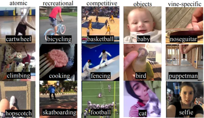
Page 1.1 Example micro-video frames. This new source of visual spans across different

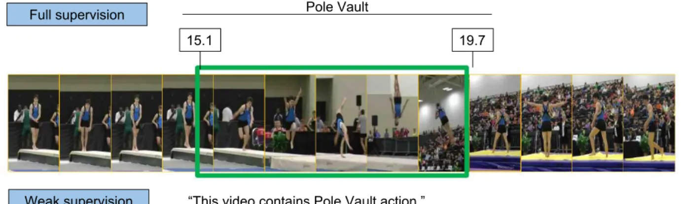
video contents: from atomic unbreakable actions to videos of a regular animal like cats. . . 2 1.2 Given an untrimmed video, the task of temporal action localization is to find

the boundaries (start and end timestamps) and the label for all the action instance. Fully-supervised models required the boundaries and action label annotations for each action instance in the video. A weaker, and often cheaper, form of supervision is video-level labels, indicating which action the video contains, but not how many instances or the locations of those instances. . . 3 2.1 Micro-videos semantically rich micro-narratives while remaining tractable to

collect, store and process. Mobile-videographers often interact with the scene and its subjects resulting in a wide range of camera viewpoints including egocentric views of activities and self-facing shots where a single individual is both the photographer and subject. Our dataset,MV-58k, includes common tags about actions and objects seen in other computer vision datasets as well as specific tags such as #noseguitar which are video-graphic styles unique to

the micro-video sharing service Vine. Distribution of videos per tag is highly skewed. . . 6 2.2 Unique temporal structure in microvideos. We visualize changes in tag label

priors over time by plotting their popularity rank as a heatmap (brighter denotes higher popularity). Note that many tags exhibit large fluctuations;

#gopdebate is ranked first during the weeks of the associated events, but

dramatically decreases otherwise. The distribution of visual appearance asso-ciated with some tags also exhibit temporal dynamics. #climbing shows large

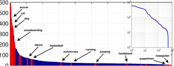
temporal variations over summer and winter months due to changes in scenery (desert rocks versus ice) and equipment. . . 8 2.3 For diagnostic purposes we construct a hand-curated dataset (MV-40)

con-taining only videos with direct visual evidence for a subset of 40 tags selected to span both common and rare tags, as shown in the long-tailed distribution. Inset shows the same distribution on a log-log scale. . . 11

(8)

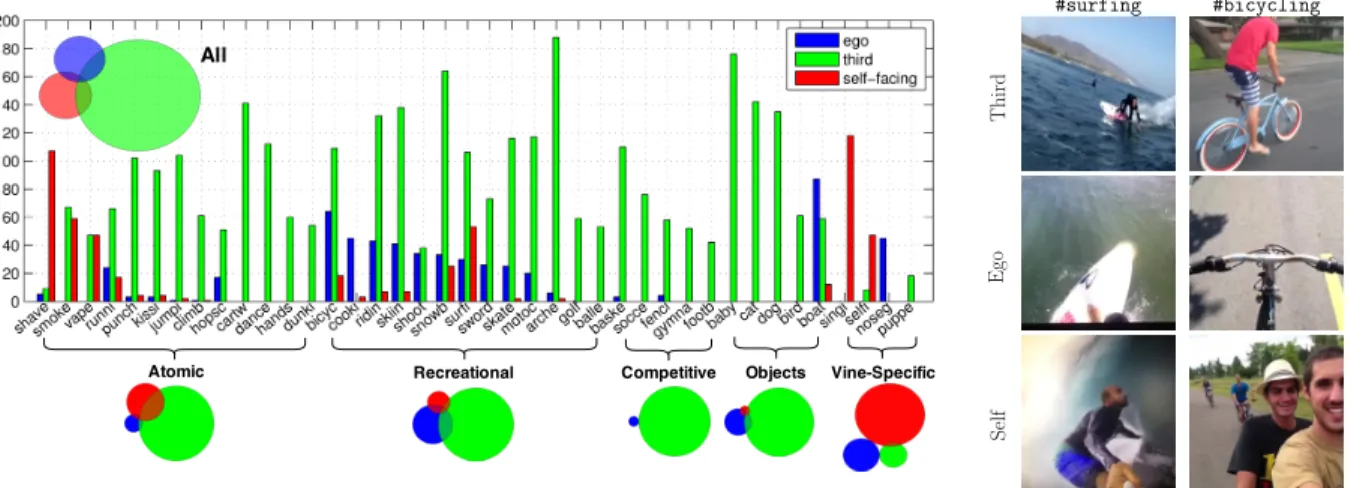
2.4 The unique viewpoints of microvideos. (a) shows the distribution of camera viewpoints annotated in MV-40. Most tags tend to be associated with third-person viewpoints. Some atomic actions such as #shave are captured with

self-facing views. Recreational sports are often in egocentric views, but this is less likely for competitive sports (soccer). Many Vine-specific tags make use of self-facing viewpoints. The Venn diagram shows that there’s a significant amount of videos that contain more than one viewpoint and some even has all 3 viewpoints. We show examples of frames with unique viewpoints on the right. 13 2.5 (a) Performance of different feature sets on MV-40 broken down by tag type

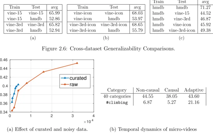
and viewpoint. (b) plots the perfomance of view-point specific tag models, exploring different choices of positive and negative data. (c) visualizes the 3-way class confusion matrix for viewpoint prediction. See text for more details. 15 2.6 Cross-dataset Generalizability Comparisons. . . 17 2.7 (a) Effect of data curation and (b) temporal dynamic of large-scale

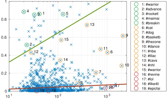
micro-videos. In (a), we compare the accuracy of models trained versus uncurated data when tested on MV-58k. Curated, clean data is often easier to train on. However, a modest amount of addtional raw training data (<2X) rivals the accuracy of a manually curated training set. In (b), we show the temporal dynamics of the micro-videos. Non-causal models perform the best but may be impractical because they must be trained on future videos. Adaptive models trained on recent videos perform better than a fixed training set because tag topics tend to temporally evolve. . . 17 2.8 Open-world tag prediction. The scatter plot shows per-tag APs vs (log) number

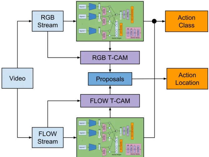
of training examples. We rank the “learnability” of a tag by the ratio of its AP to (log) number of training examples, and draw lines to loosely denote regions of easy, challenging, and unlearnable tags. Unlearnable tags appear to correspond to “stopwords” such as#revine,lol that do not capture video content. The per-tag mAPT is 0.05. . . 19

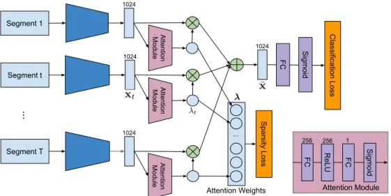
3.1 Overview of the proposed algorithm. Our algorithm takes a two-stream input— RGB frames and optical flow between frames—from a video, and performs action classification and localization concurrently. For localization, Temporal Class Activation Maps (T-CAMs) are computed from the two streams and employed to generate one dimensional temporal action proposals, from which the target actions are localized in the temporal domain. . . 21 3.2 Network architecture for our weakly supervised temporal action localization

model. We first extract feature representations for a set of uniformly sampled video segments using a pretrained network. The attention module computes class-agnostic attention weights for each segment, which are used to generate a video-level representation via weighted temporal average pooling. The representation is given to the classification module that can be trained with regular cross entropy loss with video-level labels. An`1 loss is placed on the

(9)

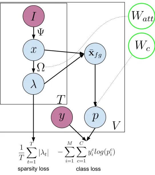
3.3 Our network is driven by two losses: a weakly supervised classification loss based on the video-level labels, y, and an unsupervised sparsity loss placed on the attention vectors, λ. . . 25 3.4 Illustration of the ground-truth temporal intervals for the ThrowDiscus class,

the temporal attentions, and the T-CAM for an example video in the THU-MOS14 dataset [48]. The horizontal axis in the plots denote the timestamps. In this example, the T-CAM values for ThrowDiscus provide accurate action localization information. Note that the temporal attention weights are large at several locations that do not correspond to the ground-truth annotations. This is because temporal attention weights are trained in a class-agnostic way. 27 3.5 Performance with respect to architecture choices. The attention module is

useful as it allows the model to explicitly focus on the important parts of input videos. Enforcing the sparsity in action recognition via`1 loss gives a

significant boost in performance. . . 33 3.6 Performance with respect to feature choices. Optical flow offers stronger cues

than RGB for action localization, and a combination of the two features leads to significant performance improvement. . . 34 3.7 Qualitative results on THUMOS14. The horizontal axis in the plots denote

time index (in seconds). (a) There are many action instances in the input video and our algorithm shows good action localization performance. (b) The appearance of the video remains similar from the beginning to end. There is little motion between each frame. Our model is still be able to localize the small time window where the action actually happens. (c) Two different actions appear in a single video and their appearances along with motion patterns are similar. Even in the case, the proposed algorithm successfully identifies two actions accurately although there are some false alarms. (d) Our results have several false positives but they are often from missing ground-truth annotations. Another source of false alarms is the similarity of the observed actions to the target action. . . 38 4.1 Using a pre-trained network, we extract the feature representation for a block

of consecutive frames (RGB or optical flows), denoted by I. The attention module maps these segment-level features,xt, into attention values, λt. These

attention values can be used to pool the segment-level features into a single foreground video-level feature representation, ¯xf g. The complements of the

attention values, 1−λ, are used to pool the segment-level features into a single background video-level feature representation, ¯xbg. The attention targets,

ˆ

λ, are created from combining the T-CAMs responses. The foreground and background video-level representations are then trained with the usual cross entropy loss with video-level labels. The self-guided loss keeps the attentions closer to the attention targets. . . 42

(10)

4.2 The detection process involves 3 steps: video-level classification probability thresholding, segment proposals and detections. First, relevant classes are selected using video-level probabilities. We threshold the attention vector and perform connected components to generate proposals. Multiple thresholds are used to obtain better segment boundaries. The proposals are then scored by the summation of the weighted-TCAM values fall into the interval. Non-maxima suppresion is done per-class to produce the final detection results. The y-axis in last figure indicates the detection score. . . 47 4.3 Compared to STPN [73], our model’s attention responses are better able to

pinpoint locations of background frames due to background modeling. The example is ’video test 001268’. . . 50 5.1 Classic methods for benchmarking algorithm performance require a test-set

with high-quality labels. While it is often easy to obtain large-scale data with noisy labels, test evaluation is typically carried out on only a small fraction of the data that has been manually cleaned-up (or “vetted”). We show that one can obtain dramatically more accurate estimates of performance by using the vetted-set to train a statistical estimator that both (1) reports improved estimates and (2) actively selects the next batch of test data to vet. We demonstrate that such an “active-testing” process can efficiently benchmark performance and and rank visual recognition algorithms. . . 53 5.2 Vetting Procedure. The figure shows the vetting procedures for the multi-label

classification (top) and instance segmentation (bottom) tasks. The annotations on the left are often incomplete and noisy, but significantly easier to obtain. These initial noisy annotations are “vetted” and corrected if necessary by a human. We quantify human effort in units of the number of image-label pairs corrected or object segment masks specified. . . 54 5.3 Standard instance segmentation benchmarks ignore unvetted data (top

path-way) when computing Average Precision. Our proposed estimator for this task computes an expected probability of a match for coarse bounding box annotations when vetted instance masks aren’t available. . . 59 5.4 Estimating P rec@K. Images at left are the top K=10 entries returned by

the system being evaluated. The image border denotes the current label and vetting status (solid blue/red = vetted positive/negative, and dotted blue/red = noisy positive/negative). Estimates of precision can be significantly improved by using a learned estimator trained on the statistics of examples that have already been vetted. Current approaches that evaluate on vetted-only or vetted+noisy labels (naive) produce poor estimates of precision (30% and 40% respectively). Our learned estimator is much closer to the true precision (63% vs 80% respectively). . . 61

(11)

5.5 Results for multi-label classification task. The figures show the mean and standard deviation of the estimated Precision@48 at different amount of annotation efforts. Using a fairly simple estimator and vetting strategy, the proposed framework can estimate the performance very closely to the true values. For references, the precision@48 averaged across classes is 20.06% and 19.88% for Microvideos and NUS-WIDE respectively. . . 63 5.6 Results for multi-label classification task. The figures show the mean and

stan-dard deviation of the estimated Precision@K at different amount of annotation efforts. Using a fairly simple estimator and vetting strategy, the proposed framework can estimate the performance very closely to the true values. . . . 64 5.7 Decoupling the effect of model change and vetting effort for NUS-WIDE. This

figure shows the reduction in estimation errors. The vertical drop at the same % vetted point indicates the reduction due to estimator quality. The slope between adjacent points indicates value of vetting examples. A steeper slope means the strategy is able to obtain a better set. In some sense, traditional active learning is concerned primarily with the vertical drop (i.e. a better model/predictor), while active testing also takes direct advantage of the slope (i.e. more vetted labels). . . 68 5.8 Results for instance segmentation. With 50% of instances vetted, our best

model’s estimation is 1% AP off from the true values with the standard deviation≤1%. A smart estimator with a smarter querying strategy can make the approach more robust and efficient. Our approach has better approximation and is less prone to sample bias compared to the standard approach(”random image”+ ”only vetted”). . . 69 5.9 Relative performance differences and their relative ranking for multiple input

systems. The left plot shows the mean squared errors between the current difference to the true difference. The right plot shows how often the ranking orders between two input algorithms are flipped. Both figures suggest that our active testing framework is a more robust and efficient approach toward comparing models. With 50% of the data vetted, standard approaches that evaluate on only vetted data (black curve) incorrectly rank algorithms 16% of the time, while our learned estimators with active vetting (red curve) reduce this error to 3% of the time. . . 70

(12)

LIST OF TABLES

Page 3.1 Comparison of our algorithm with other recent techniques on the THUMOS14

testing set. We divide the algorithms into two groups depending on their levels of supervision. Each group is sorted chronologically, from older to newer ones. STPN, including the version using UntrimmedNet features, clearly presents state-of-the-art performance in the weakly supervised setting and is even competitive with many fully supervised approaches. . . 32 3.2 Results on ActivityNet1.3 validation set. The methods with asterisk (*) report

ActivityNet challenge results, may only be available inarXiv only, and are not comparable to our algorithm directly. Although [95] shows good accuracy, it is a post-processing result from [121], making comparison difficult. . . 35 3.3 Results on the ActivityNet1.3 testing set. The methods with asterisk (*) report

ActivityNet challenge results only and are not comparable to our algorithm directly. . . 35 4.1 The addition of each loss improve the localization performance. The

improve-ments are also complement of each other as combining these losses achieves the best results. The second is copied from STPN [73] for reference. . . 48 4.2 Comparison of our algorithm with other recent techniques tested on

THU-MOS14. Our extensions gives 10% improvement over the original system [73]. We significantly outperform recent weakly supervised approaches [96, 76], 5% [email protected]. Our method is also comparable to fully-supervised methods, espe-cially in lower IoU regimes. Good performance in higher IoU requires more accurate action boundary decisions, which is difficult to obtain without the actual boundary supervisions. . . 49

(13)

LIST OF ALGORITHMS

Page 1 Active Testing Algorithm . . . 59

(14)

ACKNOWLEDGMENTS

First and foremost, I’d like to send the biggest thanks to my advisors, Deva Ramanan and Charless Fowlkes, for their supports and guidance. Through my PhD, I have learned a tremendous amount from them: from technical research skills to personal communication skills. They taught me how to be a better researcher and a better person.

I also want to thank Professor Padhraic Smyth for his time and valuable feedback on my thesis.

I want to thank my labmates, Bailey, Shu, Minhaeng, James, Sam, Golnaz, Xiangxin, Zhe, and Daeyun, for accompanying me through this journey.

Lastly, I want to thank my parents for all the supports and packed meals delievered from San Diego.

(15)

CURRICULUM VITAE

Phuc Xuan Nguyen

EDUCATION

Doctor of Philosophy in Computer Science 2019

University of California, Irvine Irvine, CA

Master of Science in Computer Sciences 2013

University of California, San Diego San Diego, CA

Bachelor of Science in Electrial Engineering and Computer Sciences 2010

(16)

REFEREED CONFERENCE PUBLICATIONS

The Open World of Micro-videos July 2016

CVPR - BigVision Workshop

Weakly Supervised Action Localization by Sparse Tem-poral Pooling Network

June 2018 CVPR

Active Testing: An Efficient and Robust Framework for Estimating Accuracy

July 2018 ICML

(17)

ABSTRACT OF THE DISSERTATION

Training and Evaluating Visual Recognition Systems with Limited Annotations By

Phuc Xuan Nguyen

Doctor of Philosophy in Computer Science University of California, Irvine, 2019

Professor Charless Fowlkes, Chair

In recent years, large-scale datasets with high-quality annotations have enabled many signifi-cant discoveries in computer vision and machine learning. However, the luxury of large-scale human annotations is not always affordable. For example, image semantic segmentation requires annotations for every pixel in an image. Similarly, action localization in untrimmed videos requires fine boundaries of action instances. The annotation effort for these tasks is prohibitively expensive to scale. What can we do in such scenarios? In this thesis, we look at different ways to circumvent this challenge. First, we examine micro-videos, a new and abundant source of visual data with user-generated metadata that could serve as web-supervision. Second, we explore weak supervision, in the context of action localization. While fine boundaries annotations of action instances are expensive and difficult to obtain, video-level labels can be cheaper and more accessible. We present two state-of-the-art systems that leveraged on this weaker form of supervision and compare them to their fully supervised counterparts. Lastly, we address the problems of accurately measuring the performance of computer vision systems with limited human annotations.

(18)

Chapter 1 Overview

Recent successes in computer vision have been largely due to large-scale, well-annotated datasets. High-quality human annotations in these datasets allows researchers to train supervised vision recognition systems with performance on par with human’s. However, it can be prohibitively expensive to scale up the annotations. For example, the authors of NUS-WIDE [20], a multi-label image classification dataset, estimates 3000 man-hours to semi-manually annotate the complete ground-truth for a relative small set of 81 concepts across 270K images. The authors of Citiscapes [21], a popular image semantic segmentation dataset, reports that an average of 1.5 hours is required to annotate a single image. In the setting of limited human annotations, it is unclear how to train and test visual recognition systems. Could we scale up the annotations in some other ways? Is there some similar form of visual data that comes with freely-available annotations? Instead of requiring tedious human efforts to label all pixels in the image, how far do we get with a weaker form of supervision, e.g. image-level annotations that tell what parts are in the image instead of their exact boundaries? Measuring performance of a system also requires large-scale annotations. How is the test performance affected by limited high-quality annotations? What if we relaxed this constraint and report the test performance on a noisier type of annotations? In this

(19)

thesis, we explore these questions.

Chapter 2 investigates webly supervision. More specifically, we closely examine a new form of visual data, called micro-videos, that are abundant freely on social media platform. These micro-videos often comes with user-generated metadata, such as tags and timestamps. Figure 1.1 shows example frames with its tags organized into different categories. We compare micro-videos characteristics with traditional video classification datasets. We extend the analysis to a larger scale: what are the effects of using raw, uncurated tags as labels versus a curated set of tags?

Figure 1.1: Example micro-video frames. This new source of visual spans across different video contents: from atomic unbreakable actions to videos of a regular animal like cats.

Chapter 3 and 4 explore weak supervision in the context of action localization. Figure 1.2 summarize the task of action localization and the annotations format for full supervision and weak supervision. Chapter 3 introduces a convolution neural network with sparse attention-weighted temporal pooling. At inference time, we extract and score temporal proposals using

(20)

flaws and proposes modifications that lead to significant improvements. The final model achieves state-of-the-art on weakly-supervised action localization and has comparable results with fully-supervised systems.

The lack of high-quality human annotations also affects the testing process. How much can you trust your performance metric when the testbed is too small? Can we trust a larger testbed with noisy labels? In Chapter 5, we introduce a framework to accurately estimate performance metrics of computer vision systems when using a cheaper, noisier labels. We re-formulate the problem as one of active testing, and examine strategies for efficiently querying a user to obtain accurate performance estimate with minimal human effort.

15.1 19.7

Pole Vault Full supervision

Weak supervision “This video contains Pole Vault action.”

Figure 1.2: Given an untrimmed video, the task of temporal action localization is to find the boundaries (start and end timestamps) and the label for all the action instance. Fully-supervised models required the boundaries and action label annotations for each action instance in the video. A weaker, and often cheaper, form of supervision is video-level labels, indicating which action the video contains, but not how many instances or the locations of those instances.

(21)

Chapter 2 The Open World of Micro-Videos

Can user-generated tags serve as a substitute to human annotations? We examine a new source of visual data which comes with a cheaper, more-readily source of annotations. As an increasingly prevalent form of media, micro-videos are time-constrained (typically 5-10 second) video clips commonly appeared on social networking sites such as Instagram, Vine, and Snapchat. Micro-videos can be interpreted as the visual analog of a character-limited micro-blogs or “tweets” [60]. An estimated 12 million micro-videos are posted to Twitter each day. The number of micro-videos produced surpasses the total inventory of YouTube every 3 months. From an applied perspective, this flood of visual data is increasingly important and has unique characteristics that are not addressed by existing computer vision methodologies and benchmarks. We further argue that the microvideo format offers unique opportunities for basic research in building systems that address lifelong learning in open-worldvisual domains.

Ease of storage/processing: A particularly attractive aspect of micro-videos is the ease of large-scale collection, storage and processing. While large-scale video datasets (EventNet [131], YouTube8M [2], Sporst1M [52]) are available, none has become a gold-stardard benchmark for video understanding. One reason is that it is notoriously challenging to store, and process

(22)

a large diverse video collection because of resource constraints. To ease the collection process, existing video collections often contain multiple snippets cropped from a few longer videos [58, 66]. This limits the diversity of the dataset. It requires hundreds of terabytes to store the complete Youtube8M dataset. To mitigate this constraint, only the video URLs and the top-level features are provided. However, URLs are often an unreliable source as videos can come and go quickly. Micro-videos, on the hands, are easy to collect and compact to store at a large-scale. The storage size of 260K videos is only 220GB.

Micro-narratives: Another intriguing aspect of micro-videos is that they arrive “ready-for-analysis”, due to the constraint that users are forced to trim content to fit within the six-second restriction. As a result, each frame of a micro-video typically has high information content compared to frames in a longer unconstrained video. This changes strategies for automated understanding and may even eliminate the need for common video preprocessing steps like keyframe or shot selection. The long format of traditional videos (such as YouTube) often forced models to operate on an sparse subsampled subset of frames and/or only use the firstX seconds of the video. Whereas, there are only 180 frames in total for a microvideo. Hence, it is within reason for models to use all the available frames for analysis.

Viewpoint: A unique technical aspect of micro-videos is camera viewpoint (Fig. 2.4). Current action datasets in computer vision focus on third-person depictions of actions, where a person(s) performing an action or activity is framed in the view. In contrast, a significant fraction of socially-driven micro-videos includeegocentricviewpoints, where the photographer is participating in the action. Another camera configuration is a self-facing viewpoint, or “selfie”, where a single user is both the photographer and subject. This is particularly interesting in the study of interactions photographers and their subjects [68]. Such diverse camera viewpoints represent new modes of video acquisition that are not typically addressed in previous work and deserve a closer look from the computer vision community.

(23)

climbing

football soccer

singing puppetman

bird cat dog

selfie baby Ato mi c Recreati o n al Co mp eti ti ve O b jects V in e-S p eci fi c bicycling basketball fencing noseguitar

cartwheel hopscotch punching

cooking skateboarding snowboarding

climbing

football soccer

singing puppetman

bird cat dog

climbing

football soccer

singing puppetman

bird cat dog

climbing

football soccer

singing puppetman

bird cat dog

climbing

football soccer

singing puppetman

bird cat dog

climbing

football soccer

singing puppetman

bird cat dog

climbing

football soccer

singing puppetman

bird cat dog

climbing

football soccer

singing puppetman

bird cat dog

climbing

football soccer

singing puppetman

bird cat dog

climbing

football soccer

singing puppetman

bird cat dog

climbing

football soccer

singing puppetman

bird cat dog

climbing

football soccer

singing puppetman

bird cat dog

climbing

football soccer

singing puppetman

bird cat dog

climbing

football soccer

singing puppetman

bird cat dog

climbing

football soccer

singing puppetman

bird cat dog

climbing

bicycling basketball baby noseguitar

cartwheel

cooking fencing bird puppetman

football

hopscotch skatboarding cat selfie

atomic recreational competitive objects vine-specific

Figure 2.1: Micro-videos semantically rich micro-narratives while remaining tractable to collect, store and process. Mobile-videographers often interact with the scene and its subjects resulting in a wide range of camera viewpoints including egocentric views of activities and self-facing shots where a single individual is both the photographer and subject. Our dataset, MV-58k, includes common tags about actions and objects seen in other computer vision datasets as well as specific tags such as #noseguitar which are video-graphic styles

unique to the micro-video sharing service Vine. Distribution of videos per tag is highly skewed.

Open-world dynamics: Micro-videos come labeled with hashtags that enable search and play an important role in social communication. These tags provide a form of supervision, automatically labeling our diverse, multi-view, pre-trimmed dataset. In contrast to existing efforts to develop top-down ontologies for activities [28] or events [132], tags form an open-world vocabulary whose usage and semantics changes dynamically over time [22]. For example, the tag #alternativefacts did not exist until recently, while the visual meaning of the

tag #apple expands whenever a new iPhone is released. Microvideos thus provide a unique

opportunity to explore learning in the open world, where distributions of visual semantics follow long-tail statistics that change time over time. Taking a bottom-up, data-driven

approach to video content semantics more accurately reflects naturally-occuring long-tail distributions that typically suppressed in hand-curated datasets. The dataset we present is thus large, has dynamic temporal variations and is continually growing is size. We analyze a snapshot as of Feb 2016 consisting of 264,327 videos with 58,243 tags.

(24)

2.1 Related Works

There is little existing work on micro-video analysis, as the medium itself is new. Redi et al. [82] explore the problem of finding creative micro-videos, inspired by similar studies of image quality assessment. Sano et al.[91] analyze the problem of detecting loop micro-videos (that are designed to be played in a continuous six-second loop). Here we focus on analyzing general properties of micro-videos, with the explicit goal of constructing a new, large-scale benchmark for temporally-evolving tag prediction.

Viewpoint modeling: A unique contribution of our dataset is the diversity of camera viewpoints. Existing video benchmarks for action recognition have focused on third-person viewpoints (e.g., HMDB [58], UCF101 [105], Hollywood-2 [69], UT-Interaction [87] and Olympic Sports [75]). Wearable cameras such as Google Glass and GoPro have spurred interest in analyzing egocentric views [29, 57, 77, 61]. Compared to existing action and egocentric datasets, our user-generated micro-videos contain a wider variety of categories (tags) and viewpoints (e.g., self-facing) with richer narrative content, even in a single clip. To understand and highlight these differences we train mixture-of-viewpoint models that specifically target viewpoint variations in dynamic micro-videos (Sec. 2.3) and carry out an extensive comparison with HMDB [58] (Sec. 5.3).

Closed vs open vocabularies: Traditionally, video datasets in computer vision have been labeled with a fixed ontology of activities or events [28, 132, 52]. An alternative perspective (popular in the multimedia community) is to formulate the problem as a multi-label tag or concept prediction task [110, 130, 7, 106, 109]. Our dataset falls into this later camp. In terms of size and diversity, the most relevant prior work appears to be Sports-1M [52] which contains 1M videos in 487 categories, and EventNet [132], which contains 95K videos labeled with 5K concepts. Our dataset already includes 2X more videos and 10X more concept tags. Unlike other video datasets, our data also includes timestamps which allow us to study

(25)

(a) tag usage dynamics

Jan-Feb 2015 July-Aug 2015

(b) appearance dynamics

Figure 2.2: Unique temporal structure in microvideos. We visualize changes in tag label priors over time by plotting their popularity rank as a heatmap (brighter denotes higher popularity). Note that many tags exhibit large fluctuations; #gopdebate is ranked first during the weeks of the associated events, but dramatically decreases otherwise. The distribution of visual appearance associated with some tags also exhibit temporal dynamics. #climbingshows large

temporal variations over summer and winter months due to changes in scenery (desert rocks versus ice) and equipment.

temporally-varying semantics, a relatively unexplored concept in vision, with the notable exception of [56]. Importantly, tag frequency distributions are highly imbalanced, following a natural long-tail distribution (Fig. 2.3). While highly imbalanced class distributions are somewhat uncommon in current vision datasets, they appear to be a fundamental aspect of life-long learning in the open-world [19]. With the advent of deep architectures that appear capable of transferring knowledge across imbalanced classes [10], we think the time is right to (re)consider learning in the open-world!

2.2 Dataset

In this section, we describe our ongoing data-collection process and analyze the statistics of micro-video tags and viewpoints that make our dataset distinct from existing video benchmarks.

(26)

Streaming dataset collection: We collect a stream of Vine videos by daily querying of Vine’s API [1]. To ensure a diverse stream, we query the 300 most popular and 300 most recent videos across multiple community-curated channels (Comedy, Sports, Musics). We typically obtain 6000 videos daily. Each video is associated with a collection of hashtags that are added to our open vocabulary. On average, a video contains 1.56 hashtags, but this statistic is skewed by the fact that nearly half the videos do not contain any tags (56%).This indirectly motivates one practical application of our dataset - automatic prediction of hashtags. We visualize our overall distribution of tags in Fig. 2.1. We useMV-58k to refer to a snapshot of this datastream collected during the period Dec-2015 to Feb-2016.

Curation: To examine the amount of “noise” in the tag stream and perform diagnostic comparisons to existing activity datasets, we manually curated a subset of 40 tags and their associated 4000 videos. We selected 40 representative tags that span both common actions as well rare tags “in-the-tail”. We “clean” this dataset by merging synonymous tags (e.g.,

#horsebackand#horsebackriding), removing mistagged (spam) videos, and removing videos

in which there was only circumstantial visual evidence for the tagged activity (see Fig. 2.3 for an example). We added additional annotations to each video including viewpoint and a dominant (tag) category. The latter allows us to recast tag prediction as a K-way classification problem, simplifying our diagnostic analysis.

We refer to this curated dataset as MV-40, and contrast this with (the fixed snapshot of) our uncurated, open-world dataset MV-58K. We organize MV-40 into broad categories of atomic actions, recreational activities, competitive sports, objects, and vine-specific. We visualize our two-level taxonomy and provide visual examples in Fig. 2.1.

Long-tail distributions: Our collection process reveals a salient property of open-world microvideos; they follow long-tail distributions of tags. This significantly complicates learning because there will be some tags for which we have little training data. While traditionally a notorious challenge for machine learning, our analysis suggests that hierarchical feature

(27)

learning (with CNNs) can learn to share, or transfer knowledge from the data-rich tags to the data-sparse tags (i.e., one-shot learning). For example, even if we have few examples of

#dunking, mid-level features learned for a data-rich tag such as #basketballmay still be

useful for the former class.

Temporal dynamics: Our openworld dataset collection has another notable property -both the frequency of tag usage and the visual appearance semantics associated with a given tag evolve over time. In probabilistic terms, we can interpret such dynamics and changes in the prior of labels (Fig. 2.2) and the likelihoodof image features conditioned on the tag label (Fig. 2.7). This suggests developing approaches for continually retraining models as new data becomes available, an idea we explore in Sec.5.3. An extreme case arises when a new tag first appears in the data stream there are no training examples available (e.g., #trump2016 did not exist until recently). In our current experiments, we simply fail to predict such tags at test time. However, we point out that the temporal appearance of new tags provides a compelling natural example ofzero-shot learning where side information about the semantic relation between tags could readily be exploited.

Viewpoint: To analyze the effect of viewpoint on recognition accuracy, we manually annotate MV-40 with the viewpoint of each video as egocentric, third-person, or self-facing. In some cases, the viewpoint changed between shots in the video in which case we record all the viewpoints present, as well as the dominant one. With this annotation we can treat viewpoint prediction as either a multi-label attribute prediction problem (where multiple viewpoints can be present in video) or a multi-class problem (where the goal is to predict the dominant viewpoint). We report the per-tag viewpoint statistics in Fig. 2.4. Interestingly, even at the shot-level, we sometimes find ambiguities in viewpoint. Some social activities (such as

#bicycling) involve both the photographer and subjects in view, suggesting a simultaneous

(28)

Figure 2.3: For diagnostic purposes we construct a hand-curated dataset (MV-40) containing only videos with direct visual evidence for a subset of 40 tags selected to span both common and rare tags, as shown in the long-tailed distribution. Inset shows the same distribution on a log-log scale.

2.3 Methods

In this section, we describe several baseline models for tag prediction and viewpoint classifi-cation. As the focus of our work is not on video feature extraction, we make use of standard feature sets. Recent results from the THUMOS evaluation benchmark [37] suggest that CNN spatial features (VGG [99]) combined with temporal motion features (IDT [115]) make for a reasonable video descriptor.

Appearance features: We found a good tradeoff in speed, storage, and accuracy with the following simple pipeline: given a video, (1) run off-the-shelf VGG-16 models [99] on 15 equally-spaced frames from a video, (2) for each frame, extract (6144-dimensional) multi-scale features across multiple layers [129], and (4) max-pool the resulting features across the 15 frames [88].

Motion features: While recent state-of-the-art results on video datasets have made use of optical flow features to represent motion features, Improved Dense Track (IDT) [115] still

(29)

offers strong signal for the learning process. This method is based on short-term tracks found from tracking interest points across frames. Various features aligned to these temporal tracks are extracted. We quantize these descriptors using K-means.

Cue-combination: We train tag classifiers that aggregate features by combining multiple kernels. We experimented extensively with various feature encodings and kernel combinations before settling on the following strategy.

We define the motion similarity with a χ2-RBF kernel:

Km(xi, xj) = exp − 1 L L X c=1 d(xc_i, xc_j) Ac ! , xc_i, xc_j ∈ R4000

where Ac is the average χ2 distance between all videos in the training data, L is the number

of motion channels, d(xc

i, xcj) is theχ2 distance between xi and xj with respect to the c-th

channel. We measure the appearance similarity between two clips using a linear kernel:

Ka(xi, xj) = PN f=1(x f i ·x f

j) summed over the N = 15 static feature channels extracted by

the CNN. We compute the similarity between two video clips xi and xj by averaging their

appearance and motion-feature similarities: K(xi, xj) = 1₂(Km(xi, xj) +Ka(xi, xj)). Given

a training vocabulary of K tags, we train K binary (one-vs-all) kernelized SVMs using the LIBSVM package [17]. Finally, we calibrate each predictor using Platt scaling [78].

Viewpoint mixtures: Different viewpoints of the same tag can have significant differences in video content, as shown in Fig. 2.1. For example, a third-person and egocentric#bicycling

video contain very different motions and appearances. To analyze such variations in the MV-40 diagnostic dataset, we train viewpoint-specific models for each tag. The final confidence associated with a tag prediction is the maximum score across the three viewpoint-specific models.

(30)

#surfing #bicycling

Third

Ego

Self

Figure 2.4: The unique viewpoints of microvideos. (a) shows the distribution of camera viewpoints annotated in MV-40. Most tags tend to be associated with third-person viewpoints. Some atomic actions such as #shave are captured with self-facing views. Recreational sports

are often in egocentric views, but this is less likely for competitive sports (soccer). Many Vine-specific tags make use of self-facing viewpoints. The Venn diagram shows that there’s a significant amount of videos that contain more than one viewpoint and some even has all 3 viewpoints. We show examples of frames with unique viewpoints on the right.

videos, we evaluate models trained with videos sampled over different temporal windows. Consider the task of predicting the labelyfor a videoxcollected at timet0 using with models

trained on a stream of timestamped training videos indexed by time. We consider models trained on three different subsets of training data:

{xt, yt :∀t} →non-causal model (2.1)

{xt, yt :t < t0} →causal model (2.2) {xt, yt:t0−∆< t < t0} →adaptive model (2.3)

where ∆ is a specified window size. The above approach can be simplified by making some assumptions about the nature of temporal variation. For example, if we assume that the popularity of tags changes over time but their appearance models do not, one can model efficiently model temporal dynamics with a statistical prior shift [90]. Intuitively, dynamics can be captured with a fixed set of posterior class predictions that are reweighted by dynamically-varying tag priors. Unfortunately, this requires access to tag priors on test data

(31)

from the future, which violates causality. Instead, we assume that tag priors vary smoothly over time, and simply use a weighted estimate of recent tags’ popularity. We found that the simple approach of applying temporally-weighted Platt rescaling (using a weighted dataset where recent videos are given more importance) outperformed an explicit prior model.

2.4 Experiments

In this section, we present an extensive set of experiments on our dataset. We focus on three sets of experiments: a diagnostic evaluation of features and viewpoints on our curated dataset (MV-40), its relation to popular benchmarks such as HMDB [58], and analysis of the open-world dynamics of MV-58K.

2.4.1 Diagnostics

First, we analyze various aspects of our dataset and recognition pipeline, focusing on the curated and annotated MV-40 subset.

Feature comparisons: We begin by comparing the performance of various combinations of our features in Fig. 2.5-(a). We observe CNN features outperform IDT in most category groups except ‘Atomic’. Trajectory-based motion and appearance-based deep features are particularly effective when combined, indicating that they capture complementary cues.

View-specific mixtures: We next evaluate the performance of view-specific tag classifiers and compare to results with a single classifier per tag. When training, one can treat clips from the same tag but different viewpoints as positive training examples (Pos), negative training examples (Neg), or such clips can be treated as neutral and ignored (Neu). Fig 2.5-(b) summarizes of the performance. When averaged over all tags, the performance increase

(32)

IDT CNN IDT+CNN All 53.90 62.13 68.82 Atomic 47.72 46.58 57.19 Recreational 60.81 69.09 76.06 Competitive 49.86 60.29 64.64 Objects 46.14 70.37 73.47 Vine-Specific 63.25 65.81 68.38 Ego 63.25 73.15 79.49 Third 51.45 60.00 67.14 Self 59.27 61.82 68.40

(a) Feature performance

Feature Pos Neu Neg IDT 62.65 64.98 64.34 CNN 58.28 60.82 60.47 IDT+CNN 68.57 70.61 70.40 (b) View-specific mixtures .61 .35 .04 .02 .95 .03 .03 .20 .77 ego third self

ego third self

(c) Viewpoint confusion

Figure 2.5: (a) Performance of different feature sets on MV-40 broken down by tag type and viewpoint. (b) plots the perfomance of view-point specific tag models, exploring different choices of positive and negative data. (c) visualizes the 3-way class confusion matrix for viewpoint prediction. See text for more details.

from view-specific mixtures is rather negligible ( 0.6% for our combined features). We also evaluate only those 11 classes for which additional views were trained. We see a small but definite improvement of 2.1%. Ignoring clips from other viewpoints (Neu) slightly increases performance.

Viewpoint prediction: We also investigate the task of viewpoint prediction: what is the viewpoint of a test video? Fig 2.5-(c) summarizes viewpoint confusions. Egocentric views are often confused with third-person and the accuracies for egocentric drops significantly. This is consistent with Fig. 2.4, which suggests many recreational activities involve both the photographer and subjects involved in the action. If we score viewpoint prediction as a multilabel problem (where each video could be labeled with more than one viewpoint), accuracy for ego, third, and self-facing jump to 92%, 90%, and 93%. This suggests the presence of any given viewpoint can be accurately predicted.

2.4.2 Cross-dataset Generalizability

We compare the overall difficulties and cross-dataset generalizability between our dataset and a standard action recognition benchmark, HMDB-51 [58]. Overall, the average accuracy on vine-15 is lower than HMDB (65.99% vs. 71.27%), suggesting that micro-videos are

(33)

more challenging. To quantify how biased or general a dataset may be, we measure the ‘performance drop’ between different datasets [107]. The cross-dataset drop for Vine data (13%) is significantly lower than HMDB (26.75%), which suggests models trained on

micro-videos are more able to generalize to other datasets.

Viewpoint: One might hypothesize that since HMDB contains mostly third-person views, it won’t generalize to the other viewpoint in our data. To test this, we extract a smaller subset vine-3rd containing only third-person viewpoints. Fig 2.6-(g) shows that vine-3rd is more similar to HMDB, as models trained on HMDB data perform better on vine-3 than vine-15. However, performance drop for models trained on vine-3rd is still significantly smaller than those trained on HMDB (12.88% vs. 24.4%). This suggests that even accounting for viewpoint, our videos still generalize better than HMDB.

Temporally iconic videos: The concept of “iconic views” in object recognition refers to “easy” images with a clear and distinctive depiction of an object, often close cropped or in an uncluttered setting without occlusion. We apply this notion to video, defining atemporally iconic depiction of a tag as one where temporal clutter has been removed by trimming down the video clip to focus on the core action. We manually segment each video in vine-15to derive an iconic versionvine-icon and use vine-3rd-iconto denote the third-person subset. Fig. 2.6 reveals that vine-icon and vine-3rd-icon are more similar to HMDB (following our previous analysis). However, their cross-dataset performance drops (14.06% and 12.86% respectively) are still significantly smaller than the drop by models trained HMDB data (25.35% and 21.89%). To summarize, even though third-person and temporal iconic-ness accounts for much of the difference between HMDB and our dataset, our micro-videos can still generalize better.

(34)

Train Test avg

vine-15 vine-15 65.99

vine-15 hmdb 52.86

vine-3rd vine-3rd 65.82

vine-3rd hmdb 52.94

Train Test avg

vine-icon vine-icon 68.03

vine-icon hmdb 53.97

vine-3rd-icon vine-3rd-icon 68.65

vine-3rd-icon hmdb 55.79

Train Test avg

hmdb hmdb 71.27 hmdb vine-15 44.52 hmdb vine-3rd 46.87 hmdb vine-icon 45.92 hmdb vine-3rd-icon 49.38 (a) (b) (c)

Figure 2.6: Cross-dataset Generalizability Comparisons.

×104 0 1 2 3 4 0.34 0.36 0.38 0.4 0.42 0.44 0.46 curated raw

(a) Effect of curated and noisy data.

Category Non-causal Causal Adaptive 40 categories 44.55 38.05 43.60

#climbing 6.87 5.27 21.16

(b) Temporal dynamics of micro-videos

Figure 2.7: (a) Effect of data curation and (b) temporal dynamic of large-scale micro-videos. In (a), we compare the accuracy of models trained versus uncurated data when tested on MV-58k. Curated, clean data is often easier to train on. However, a modest amount of addtional raw training data (<2X) rivals the accuracy of a manually curated training set. In (b), we show the temporal dynamics of the micro-videos. Non-causal models perform the best but may be impractical because they must be trained on future videos. Adaptive models trained on recent videos perform better than a fixed training set because tag topics tend to temporally evolve.

2.4.3 Micro-videos at Large

In this section, we analyze properties of our open-world MV-58K dataset.

Curated vs raw data: When comparing models trained on curated versus open-world data (Fig. 2.7), given a fixed amount of training data, curated data performs better. However, the performance gap is closed quickly when trained with more (<2x) raw data. This suggests that instead of spending efforts on cleaning the data, collecting additional raw, noisy data will achieve the similar results. This is promising as it is practically a lot easier to collect 2x more raw data than cleaning the current data.

(35)

Temporal dynamics: We now examine the time-varying properties of micro-video content and tags (Fig. 2.7). We find that the problem of causal prediction (where one only has access to data from the past) is much harder than the non-causal counterpart, suggesting that micro-videos are not “IID” over time. Current benchmarks are assuming the independence between samples over time and, hence, are likely to be over-estimating real-world performance on streaming data. Much of this temporal variation can be explained by fluctuations of tag popularity, whose degree of variation can vary dramatically across classes.

Open vocabularies: We now move beyond our 40 selected tags to evaluation of an open-world vocabulary. We treat this as a multi-label classification task (since videos can be naturally labeled with many tags). We report the per-tag mean average precision (mAP). Fig. 2.8 shows the per-tag mAP as a function of training-set size in. We tend to see different performance regimes. “Easy” tags perform well even with little training data, likely due to a characteristic appearance that is easy to learn from little training data (#cavs). “Challenging” tags appear to contain appearance variation, but are learnable with additional data (#dogs). “Unlearnable” tags remain near-zero AP even given lots of training data (#revine). We posit

that these can be treated as stopwords that fail to capture much semantic meaning of the video.

2.5 Conclusions

We introduce a open-world dataset of micro-videos, which lie in a regime between single images and typical videos, allowing for easy capture, storage, and processing. They contain micro-narratives captured from viewpoints typically not studied in computer vision. Because they are naturally diverse, pre-trimmed, and user-annotated, they can be used a live testbed for open-world evaluation of video understanding systems.

(36)

101 102 103 0 0.2 0.4 0.6 0.8 1 1 2 3 4 5 6 7 8 9 10 11 12 13 14 15 16 17 18 19 1: #warrior 2: #advance 3: #rocketl 4: #maimai 5: #breakin 6: #cat 7: #dog 8: #basketb 9: #thezone 10: #dance 11: #nba 12: #lilac 13: #cavs 14: #nhl 15: #warrior 16: #revine 17: #lol 18: #like4li 19: #epicfai

Figure 2.8: Open-world tag prediction. The scatter plot shows per-tag APs vs (log) number of training examples. We rank the “learnability” of a tag by the ratio of its AP to (log) number of training examples, and draw lines to loosely denote regions of easy, challenging, and unlearnable tags. Unlearnable tags appear to correspond to “stopwords” such as#revine,lol that do not capture video content. The per-tag mAPT is 0.05.

(37)

Chapter 3 Weakly supervised Action

Localization by Sparse Temporal

Pooling

In the previous chapter, we explored the possibilities of using web supervision as a replacement for human annotations. In this chapter, we explore weak supervision in the context of action localization. Instead of requiring the effort-intensive annotation effort of labeling the boundaries for actions in videos, we investigate training with a weaker form of supervision: video-level labels. For this task, the objective is to find the boundaries and class of the action instances given an untrimmed video. Human annotation effort for constructing the training data for this task include watching uncut videos and identifying the action boundaries for each of the interested classes. The process of identifying action boundaries can be very noisy and time-consuming. An alternative approach is to train with weak supervision: the model can only observe video-level labels indicating whether the video contains certain actions. These types of annotation efforts are significantly less intensive than pinpointing the exact boundaries of every action instance within a video.

(38)

FLOW

Stream

Action

Class

FLOW T-CAM

Proposals

Action

Location

RGB

Stream

RGB T-CAM

Video

Figure 3.1: Overview of the proposed algorithm. Our algorithm takes a two-stream input—RGB frames and optical flow between frames—from a video, and performs action classification and localization concurrently. For localization, Temporal Class Activation Maps (T-CAMs) are computed from the two streams and employed to generate one dimensional temporal action proposals, from which the target actions are localized in the temporal domain.

3.1 Related Works

Action recognition aims to identify a single or multiple actions per video and is often formulated as a simple classification problem. Before deep learning started being actively used, the algorithm based on improved dense trajectories [116] presented outstanding performance. When it comes to the era of deep learning, convolutional neural networks have been widely used. Two-stream networks [98] and 3D convolutional neural networks (C3D) [108] are popular solutions to learning video representations and these techniques, including their variations, are extensively used for action recognition. Recently, a combination of two-stream

(39)

networks and 3D convolutions, referred to as I3D [16], was proposed as a generic video representation learning method. On the other hand, many algorithms develop techniques to recognize actions based on existing representation methods [119, 122, 30, 34, 31, 94].

Action localization is a different from the problem of action recognition, because it requires the detection of temporal or spatiotemporal volumes containing target actions. There are various existing methods based on deep learning including structured segment network [139], contextual relation learning [103], multi-stage CNNs [97], temporal association of frame-level action detections [35], and techniques using recurrent neural networks [133, 67]. Most of these approaches rely on supervised learning and employ temporal or spatio-temporal annotations to train the models. To facilitate action detection and localization, many algorithms use the action proposals [15, 25, 117] technique, which is an extension of object proposals for object detection in images.

There are only a few approaches based on weakly supervised learning that rely solely on video-level class labels to localize actions in temporal domain. UntrimmedNet [118] learns attention weights on precut video segments using a temporal softmax function and thresholds the attention weights to generate action proposals. The algorithm improves the video-level classification performance. However, only using class-agnostic attention weights for action proposal is clearly not optimal and the use of the softmax function across proposals may not be effective to detect multiple instances. Hide-and-seek [102] proposes a technique that randomly hides regions to force residual attention learning and thresholds class activation maps at inference time for weakly supervised spatial object detection and temporal action localization. While working well at spatial localization tasks, this method fails to show satisfactory performance in temporal action localization tasks. Both algorithms are motivated by the recent success of weakly supervised object localization in images. In particular, the formulation of UntrimmedNet for action localization heavily relies on the idea proposed in [11]. There are some other approaches [12, 46, 85] that learn to localize or segment actions in a

(40)

... Segment 1 Segment t FC Sigmoid Classification Loss ... Segment T Attention Module Sparsity Loss 1024 1024 1024 Attention Weights Attention Module Attention Module 1024 Sigmoid Attention Module ReLU 256 1 FC FC 256

Figure 3.2: Network architecture for our weakly supervised temporal action localization model. We first extract feature representations for a set of uniformly sampled video segments using a pretrained network. The attention module computes class-agnostic attention weights for each segment, which are used to generate a video-level representation via weighted temporal average pooling. The representation is given to the classification module that can be trained with regular cross entropy

loss with video-level labels. An`1 loss is placed on the attention weights to enforce sparse attentions.

weakly supervised setting by exploiting the temporal order of subactions during training. The main objective of these studies is to find the boundaries of sequentially presented subactions, while our approach aims to extract temporal intervals of full actions from input videos.

In terms of datasets, there are several publicly available datasets for action recognition including UCF101 [104], Sports-1M [53], HMDB51 [59], Kinetics [54] and AVA [38]. The videos in these datasets are trimmed so that the target actions appear throughout each clip. In contrast, THUMOS14 dataset [48] and ActivityNet [42] provide untrimmed videos that contain background frames and temporal annotations about which frames are relevant to the target actions. Note that each video in THUMOS14 and ActivityNet may have multiple actions happening in a single frame.

(41)

3.2 Proposed Algorithm

We claim that an action can be recognized from a video by identifying a set of key segments presenting important action components. So we design a neural network that learns to measure the importance of each segment in a video and automatically selects a sparse subset of representative segments to predict the level class labels. Only ground-truth video-level class labels are required for training the model. For action localization at inference time, we first identify relevant classes in each video and then generate temporal action proposals from temporal class activations and attentions to find the temporal locations of each relevant classes. The network architecture for our weakly supervised action recognition component is illustrated in Figure 3.2. We describe each step of our algorithm in the following sections.

3.2.1 Action Classification

To predict class labels in each video, we sample a set of segments and extract feature representations from each segment using pretrained convolutional neural networks. Each feature vector is then fed to an attention module that consists of two fully connected (FC) layers and a ReLU layer located between the two FC layers. The output of the second FC layer is given to a sigmoid function that ensures the generated attention weights are between 0 and 1. These class-agnostic attention weights are then used to modulate the temporal average pooling—a weighted sum of the feature vectors—to create a video-level representation. We pass this representation through an FC and sigmoid layers to obtain class scores.

Formally, let It represent a chunk of images (either RGB or flow) at centered timestamp

t. We assume there exists a function Ψ that maps these frame or flow chunks into feature representation xt ∈ Rd. For the rest of this chapter, we assume a fixed Ψ during the training process, i.e. we freeze the weights in the layers implementation of Ψ. With a fixed

(42)

class loss

sparsity loss

Figure 3.3: Our network is driven by two losses: a weakly supervised classification loss based on the

video-level labels,y, and an unsupervised sparsity loss placed on the attention vectors, λ.

feature extractor, a dataset with C classes for weakly-supervised action localization is a set, {xi,t}Tt=1i , yi

M

i=1, containingM number of videos and each video contains Ti number of

feature vectors xi,t, and M number of video-level groundtruth label vectors, y∈ {0,1}C.

The attention function, Ω, converts this m-dimensional feature vector into a single real scalar,

λt = Ω(xt), between 0 and 1. This function is implemented using two fully-connected (FC)

layers, ReLU layer located between the two FC layers, and a sigmoid function at the end. The video level representation, denoted by ¯x, corresponds to an attention weighted temporal

(43)

average pooling, which is given by ¯ x= T X t=1 λtxt, (3.1)

whereλ= (λ1, . . . , λT)>is a vector of scalar outputs from the attention module. The attention

weight vectorλ is defined in a class-agnostic way, which is useful to identify segments relevant to all the actions of interest for estimating the temporal intervals for action candidates later.

Feeding this foreground video-level feature representation to an FC layer, parameterized by

Wclass∈ RC+1×D and normalized to a probability using an activation function (sigmoid or

softmax), we obtain

p=σ(W_classT x)¯ , (3.2)

whereσ is an activation function of choice (softmax or sigmoid). The foreground classification loss is the defined via regular cross-entropy loss,

Lclass =− M X i=1 C X c

yi,clog(pf gi,c) (3.3)

To enforce the fact that only a small fraction number of frames in the video should be active, we integrate a sparsity loss on attention weights,

Lsparsity = M X i 1 Ti Ti X t |λt|. (3.4)

The loss function in the proposed network is composed of two terms, the classification loss and the sparsity loss, which is given by

(44)

where β is a hyperparameter to control the trade-off between the two terms.

Because of the sigmoid function and the `1 loss, all the attention weights tend to have values

close to either 0 or 1. Note that integrating the sparsity loss is aligned with our claim that an action can be recognized with a sparse subset of key segments in a video. Figure 3.3 summarizes our notations.

3.2.2 Temporal Class Activation Mapping

Groundtruth Attention

T-CAM

Figure 3.4: Illustration of the ground-truth temporal intervals for the ThrowDiscus class, the

temporal attentions, and the T-CAM for an example video in the THUMOS14 dataset [48]. The horizontal axis in the plots denote the timestamps. In this example, the T-CAM values for

ThrowDiscus provide accurate action localization information. Note that the temporal attention weights are large at several locations that do not correspond to the ground-truth annotations. This is because temporal attention weights are trained in a class-agnostic way.

To identify the time intervals corresponding to target actions, we extract a number of action interval candidates. Based on the idea in [141], we derive a one dimensional class-specific activation map in the temporal domain, referred to as the Temporal Class Activation Map (T-CAM). Let wc(k) denote the k-th element in the weight parameter wc of the final fully

(45)

The input to the final sigmoid layer for class cis sc= m X k=1 wc(k)¯x(k) = m X k=1 wc(k) T X t=1 λtxt(k) (3.6) = T X t=1 λt m X k=1 wc(k)xt(k). T-CAM, denoted by at = (a1t, a2t, . . . , aCt )

>_{, indicates the relevance of the representations to}

each class at time step t, where each elementac

t for class c(c= 1, . . . , C) is given by

ac_t =

m X

k=1

wc(k)xt(k). (3.7)

Figure 3.4 illustrates an example of the attention weights and the T-CAM outputs in a video given by the proposed algorithm. We can observe that the discriminative temporal regions are effectively highlighted by the attention weights and the T-CAMs. Also, some temporal intervals with large attention weights do not correspond to large T-CAM values because such intervals may represent other actions of interest. The attention weights measure the generic actionness of temporal video segments while the T-CAMs present class-specific information.

3.2.3 Two-stream CNN Models

We employ the recently proposed I3D model [16] to compute feature representations for the sampled video segments. Using multiple streams of information such as RGB and optical flow has become a standard practice in action recognition and detection [16, 32, 98] as it often provides a significant boost in performance. We also train two action recognition networks separately with identical settings as illustrated in Figure 3.2 for the RGB and the flow stream.

(46)

Note that our I3D networks are pretrained on the Kinetics dataset [54], and we only use it as a feature extraction machine without any fine-tuning on our target datasets. Our two-stream networks are then fused to localize actions in an input video. The procedure is discussed in the following subsection.

3.2.4 Temporal Action Localization

For an input video, we identify relevant class labels based on video-level classification scores (Section 3.2.1). For each relevant action, we generate temporal proposals, i.e. one-dimensional time intervals, with their class-specific confidence scores, corresponding to segments that potentially enclose the target actions.

To generate temporal proposals, we compute the T-CAMs for both the RGB and the flow streams, denoted by ac

t,RGB and act,FLOW respectively, based on (3.7) and use them to derive

the weighted T-CAMs, ψc

t, RGB and ψct, FLOW as

ψ_t,c_RGB =λt,RGB·sigmoid(act,RGB) (3.8)

ψ_t,c_FLOW =λt,FLOW·sigmoid(act,FLOW). (3.9)

Note that λt is an element of the sparse vector λ, and multiplying λt can be interpreted as a

soft selection of the values from the following sigmoid function. Similar to [141], we threshold the weighted T-CAMs, ψc

t,RGB and ψt,cFLOW to segment these signals. The temporal proposals

are then the one-dimensional connected components extracted from each stream. It is intuitive to generate action proposals using the weighted T-CAMs, instead of directly from the attention weights, because each proposal should contain a single kind of action. Optionally, we linearly interpolate the weighted T-CAM signals between sampled segments before thresholding to improve the temporal resolution of the proposals with minimal computation addition.

Training and Evaluating Visual Recognition Systems with Limited Annotations

UC Irvine

UC Irvine Electronic Theses and Dissertations

DEDICATION

TABLE OF CONTENTS

LIST OF FIGURES

LIST OF TABLES

LIST OF ALGORITHMS

ACKNOWLEDGMENTS

CURRICULUM VITAE

Phuc Xuan Nguyen

ABSTRACT OF THE DISSERTATION

Chapter 1

Overview

Chapter 2

The Open World of Micro-Videos

2.1

Related Works

2.2

Dataset

2.3

Methods

2.4

Experiments

2.4.1

Diagnostics

2.4.2

Cross-dataset Generalizability

2.4.3

Micro-videos at Large

2.5

Conclusions

Chapter 3

Weakly supervised Action

Localization by Sparse Temporal

Pooling

FLOW

Stream

Action

Class

FLOW T-CAM

Proposals

Action

Location

RGB

Stream

RGB T-CAM

Video

3.1

Related Works

3.2

Proposed Algorithm

3.2.1

Action Classification

class loss

sparsity loss

3.2.2

Temporal Class Activation Mapping

3.2.3

Two-stream CNN Models

3.2.4

Temporal Action Localization