Committee-based Active Learning for Surrogate-Assisted Particle Swarm Optimization of Expensive Problems

Committee-based Active Learning for

Surrogate-Assisted Particle Swarm Optimization of

Expensive Problems

Handing Wang,

Member, IEEE,

Yaochu Jin,

Fellow, IEEE,

John Doherty

Abstract—Function evaluations of many real-world optimiza-tion problems are time or resource consuming, posing a serious challenge to the application of evolutionary algorithms to solve these problems. To address this challenge, the research on surrogate-assisted evolutionary algorithms has attracted increas-ing attention from both academia and industry over the past decades. However, most existing surrogate-assisted evolutionary algorithms either still require thousands of expensive function evaluations to obtain acceptable solutions, or are only applied to very low-dimensional problems. In this paper, a novel surrogate-assisted particle swarm optimization inspired from committee-based active learning is proposed. In the proposed algorithm, a global model management strategy inspired from committee-based active learning is developed, which searches for the best and most uncertain solutions according to a surrogate ensemble using a particle swarm optimization algorithm and evaluates these solutions using the expensive objective function. In addition, a local surrogate model is built around the best solution obtained so far. Then a particle swarm optimization algorithm searches on the local surrogate to find its optimum and evaluates it. The evolutionary search using the global model management strategy switches to the local search once no further improvement can be observed, and vice versa. This iterative search process continues until the computational budget is exhausted. Experimental results comparing the proposed algorithm with a few state-of-the-art surrogate-assisted evolutionary algorithms on both benchmark problems up to 30 decision variables as well as an airfoil design problem demonstrate that the proposed algorithm is able to achieve better or competitive solutions with a limited budget of hundreds of exact function evaluations.

Index Terms—particle swarm optimization, expensive prob-lems, surrogate, model management, active learning.

I. INTRODUCTION

As a powerful optimization tool, evolutionary algorithms (EAs) are able to solve problems that cannot be easily handled by conventional mathematical programming techniques and have found many successful real-world applications [1]. In

This work was supported in part by an EPSRC grant (No. EP/M017869/1) on “Data-driven surrogate-assisted evolutionary fluid dynamic optimisation”, in part by the National Natural Science Foundation of China (No. 61590922) and in part by the Joint Research Fund for Overseas Chinese, Hong Kong and Macao Scholars of the National Natural Science Foundation of China (No. 61428302).

H. Wang is with the Department of Computer Science, University of Surrey, Guildford GU2 7XH, U.K. (e-mail: [email protected]).

Y. Jin is with the Department of Computer Science, University of Surrey, Guildford GU2 7XH, U.K. (e-mail: [email protected]). He is also affiliated with the State Key Laboratory of Synthetical Automation for Process Industries, Northeastern University, Shenyang, China. (Corresponding author) J. Doherty is with the Department of Mechanical Engineering Sciences, University of Surrey, Guildford GU2 7XH, U.K. (e-mail: [email protected]).

the real world, however, it is more often than not that quality evaluations involve computationally expensive numerical sim-ulations or costly experiments [2]. In some cases, simsim-ulations in multiple fidelity levels are available for evaluations [3], [4]. For example, two- and three-dimensional computational fluid dynamic (CFD) simulations are subject to a trade-off between fidelity and computational cost [5]. Multi-fidelity optimization methods take the full advantages of different fidelity levels [6]. However, the simulation model with the lowest fidelity level may still be computationally expensive, e.g., one single CFD simulation takes from minutes to hours [7]. Such expensive function evaluations cannot be afforded by EAs, which typically require tens of thousands fitness evalua-tions. To overcome this barrier, surrogate-assisted evolutionary algorithms (SAEAs) have been developed where part of the expensive fitness evaluations are replaced by computationally cheap approximate models, often known as meta-models or surrogates [5], [8].

SAEAs have become a popular approach to optimization of the real-world expensive problems [9], [10], due to their effectiveness in reducing the computational cost to a relatively low budget, provided that the computational cost for building surrogates takes much less time than that for the exact function evaluations (FEs). Given certain amount of data, a single model [11] or multiple models [12], [13] can be employed to estimate the fitness of candidate solutions. In the litera-ture, polynomial regression (PR) models [14], support vector machines (SVMs) [15], radial basis function (RBF) networks [16], [17], artificial neural networks (ANN) [9], and Gaussian processes (GP), also known as Kriging [18], [19] have been used to construct surrogates.

As indicated in [8], [9], model management plays a key role in making the most use of surrogate models given a limited computational budget. According to the discussions detailed in [10], various model management strategies are needed for online and offline data-driven SAEAs, mainly depending on the amount of given data and the availability of new data. For offline SAEAs, no new data can be made available during the optimization and the model management strategy considerably varies depending on whether the amount of given data is big [10] or small [20]. For online SAEAs, it is usually assumed that the model management strategy is able to actively identify a limited number of new candidate solutions to be evaluated using the expensive fitness function. In this paper, we assume that the optimization algorithm is allowed to evaluate a small number of selected solutions during optimization and therefore

we focus on developing a new model management strategy that identifies new solutions to be evaluated that can most effectively accelerate the convergence process.

Most earlier model management strategies employ a gen-eration based method [21], [22]. In gengen-eration based model management approaches, the key question is to adapt the frequency in which the real fitness function is used. For example, a strategy inspired from the trust region method was proposed in a surrogate-assisted genetic algorithm [22], while the average approximation error of the surrogate during one control cycle was used in an evolution strategy with covariance matrix adaptation to adjust the frequency of using the real objective function [9].

By contrast, individual based model management [9], [23] focuses on determining which individuals need to be evaluated within each generation. The most straightforward criterion is to evaluate solutions that have the best fitness according to the surrogate [9], [21], because these solutions might improve the accuracy of the model in the promising region of search space and lead to better solutions on the basis of the updated surrogate model. An alternative criterion is to select solutions whose estimated fitness is the most uncertain [23], [24]. Eval-uation of these solutions can not only encourage exploration but most effectively enhance the accuracy of the surrogate as well [5]. To estimate uncertainty in fitness estimation, the average distance between a solution and the training data can be adopted [23]. Since Kriging models are able to provide uncertainty information in the form of a confidence level of the predicted fitness [25], they have recently become very popular in SAEAs. To take advantage of the uncertainty information provided by the Kriging models, various model management critera, also known as infill sampling criteria in the Kriging-assisted optimization, have been proposed in SAEAs, such as probability of improvement (PoI) [26], [27], expected improvement (ExI) [26], [28], and lower confidence bound (LCB) [11].

So far most SAEAs have been developed to tackle small to medium-sized (up to 30 decision variables) expensive opti-mization problems with few exceptions [29], [30], [31], [32], partly because a majority of real-world expensive optimization problems have a medium-sized decision variables [11], and partly because most surrogates are not able to perform well for high-dimensional problems with limited training data. Nev-ertheless, existing SAEAs typically still require a large number of expensive FEs to obtain an acceptable solution. For exam-ple, the ensemble-based generalized surrogate single-objective memetic algorithm (GS-SOMA) [33] needs 8000 exact FEs for 30-dimensional single-objective benchmark problems, the PoI-based surrogate-assisted genetic algorithm with global and local search strategy (SAGA-GLS) [27] costs 6000 exact FEs on 20-dimensional single-objective benchmark problems, and the Gaussian process surrogate model assisted evolutionary algorithm for medium-scale expensive problems (LCB-based GPEME) [11] uses 1000 exact FEs for 30- and 50-dimensional single-objective benchmark problems. Such a large number of expensive FEs, although already greatly reduced compared to those used in the evolutionary optimization literature, is not practical for many extremely expensive problems. In this

paper, we aim to develop a new algorithm that is able to obtain acceptable solutions to medium scale expensive optimization problems with a budget of hundreds of exact FEs. To this end, a new model management strategy is proposed by borrowing ideas from committee-based active learning [34], [35] that actively queries new training data to most efficiently improve the approximation quality of the current model without signifi-cantly increasing the size of training dataset. More specifically, we employ a global model management strategy that aims to find the most uncertain and the best solutions for evaluation suggested by an ensemble surrogate using a particle swarm optimization (PSO) algorithm [36]. On top of this global model management strategy, we also introduce a local model management strategy that searches for the optimum of a local surrogate for evaluation.

The rest of this paper is organized as follows. Section II elaborates the connection between model management and active learning that has motivated this work. Section III de-scribes the details of the proposed algorithm. The comparative experimental results on benchmark problems are presented in Section IV, followed by an application of the proposed algorithm to an airfoil design optimization problem in Section V. Section VI concludes this paper with a summary of this paper and a discussion of future work.

II. MOTIVATIONS

Model management in online SAEAs aims to reduce the number of exact FEs while still being able to achieve high-quality solutions [8]. In SAEAs, the training dataset Dt = {hx1, y1i, ...,hxt, yti}storestsolutions, including their

deci-sion variables and fitness value evaluated with the expensive fitness function denoted in Equation (1), where x is a d-dimensional decision vector. Using Dt, a surrogate model,

which is an approximation of the expensive fitness function, can be constructed, as denoted in Equation (2). The errorεin Equation (3) describes the difference between the expensive fitness function and the surrogate.

y=f(x) (1)

ˆ

y= ˆf(x, Dt) (2)

f(x) = ˆf(x, Dt) +ε(x) (3)

The main target of model management is to identify a new candidate solution xt+1 to be evaluated for its exact fitness

value yt+1 using the expensive exact objective function [8],

[28]. Then, the new sample will be added to the databaseDt,

leading to an updated datasetDt+1 as expressed in Equation

(4):

Dt+1=Dt∪ hxt+1, yt+1i (4)

Typically, two criteria are used to select new candidate solutions to be evaluated and then added to Dt for updating

the surrogate. The first criterion is to select the optimum of the surrogate modelfˆ(x, Dt), as described in Equation (5).

xf_t+1= arg min

x

ˆ

With xf_t+1, the updated surrogatefˆ(x, Dt+1)will learn more

details about the fitness landscape around xf_t+1, which offers the search algorithm an opportunity to exploit the promising area round the optimum.

The second criterion is to select the solution whose predic-tion given by the surrogate is the most uncertain,fˆ(x, Dt), as

shown in Equation (6), implying that there are few samples near this solution inDt:

xu_t+1= arg max

x

U( ˆf(x, Dt)), (6)

where U( ˆf(x, Dt)) is the uncertainty measurement of

ˆ

f(x, Dt). By evaluating the most uncertain solution and

adding it to the database, the search algorithm will be able to explore a new region in the decision space based on the updated surrogate model.

In most SAEAs, two criteria are usually combined into one criterion, e.g., PoI, ExI, and LCB as discussed in Section I, which may make it difficult to strike a proper balance between exploration and exploitation. To address the above issue, we resort to active learning [34] that has become very popular recently in the machine learning community. One of the existing query strategies of active learning is to minimize the expected error of a model by proposing a small number of new queries (new sample points). Because of the active queries, the size of training dataset of active learning can often be much smaller than the required size in normal supervised learning [37].

There are various query strategies in active learning [37]. Among them, query by committee (QBC) [38] is a simple yet very effective active learning approach [39], which can be applied to both classification and regression problems [35]. QBC involves a committee of models that are all trained by the dataset Dt. Each model can vote on the output of a

series of query candidates, then the query with the maximum disagreement is added to the training dataset. It is believed that such query strategy can efficiently enhance the accuracy. It is clear that model management in SAEAs and making queries in active learning share similar questions to answer. They are both concerned with the efficient use of limited data to enhance the quality of models as much as possible. In this paper, we aim to borrow the ideas from active learning to improve the efficiency of model management. To be exact, we select solutions to be evaluated and added to the dataset for surrogate training by adopting a similar strategy used in QBC.

III. SURROGATE-ASSISTEDPARTICLESWARM

OPTIMIZATION VIACOMMITTEE-BASEDACTIVE

LEARNING

A. The Overall Framework

The canonical PSO algorithm is an efficient single-objective optimizer inspired from swarm behaviors of social animals such as fish schools and bird flocking [40]. Assisted by surrogate models, PSO has been employed to cope with real-world expensive optimization problems [41], such as the groundwater bioremediation problem [42] and aerodynamic

shape design problem [43]. Most existing surrogate-assisted PSO algorithms use a single surrogate model.

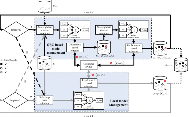
A novel surrogate-assisted PSO with the help of committee-based active learning, termed CAL-SAPSO, is proposed in this section. A generic diagram of the overall algorithm is presented in Fig. 1. The PR, RBF, and Kriging models are employed as the surrogate ensemble. To update the surrogate ensemble, samples are chosen to be evaluated using three different criteria during the iterations in CAL-SAPSO. Those criteria are controlled by two model management strategies: one based on QBC that globally searches for the most uncer-tain and the best solution of the current surrogate, respectively, while the other searches for the best solution of a local surrogate around the current optimum.

In the QBC based model management, two criteria, i.e., uncertainty and performance, are adopted to add new infilling samples into the dataset. The uncertainty based criterion measures the disagreement among the outputs of the ensemble members, while the performance based criterion is the fitness estimated by the surrogate. Both criteria are based on the global ensemble surrogate model. In the local model manage-ment, the estimated fitness is the only criterion. However, the fitness is estimated using the local surrogate, which is based on the ensemble surrogate model built using data around the current optimum.

In the proposed algorithm, we employ a PSO variant with linear weight adaption [36] to optimize those three criteria, maximizing either the fitness or uncertainty, which can be viewed as three different optimization problems.

Before the optimization starts, Latin hypercube sampling (LHS) [44] is applied to initialize the dataset with5dsolutions, where d is the dimension of the decision space, evaluated using the expensive fitness function (denoted asDInitial) for

building the initial surrogate in Fig. 1.

The algorithm starts with the QBC based model manage-ment, and switches to the local model management whenever no further improvement can be achieved. Vice versa, the algorithm switches back to the QBC based model management whenever the fitness can no longer be improved using the local surrogate model. The whole algorithm terminates when the maximum number of expensive FEs is exhausted, which is denoted as DT ermination in Fig. 1. Like the setting in [2], a

maximum number of 11dexact FEs in total can be used for CAL-SAPSO.

In the following, we will present the details of the optimizer, the QBC based model management, and the local model management.

B. Particle Swarm Optimization

In the canonical PSO algorithm [40], each individual solu-tionxin generationgupdates its position by the velocityvas Equation (7), which is based on the previous velocity, the best solution found so far by each particle (personal best) xpbest, and the best of the personal best solutions (global best)xgbest

as shown in Equation (8), where r1 and r2 are two random

numbers in [0,1], c1 andc2 are set to 1.49445 as suggested

in [45].

Fig. 1. A generic diagram of the surrogate-assisted PSO based on committee-based active learning.

vg+1=wgvg+c1r1(xpbest−xg) +c2r2(xgbest−xg) (8)

In the PSO with linear weight adaptation, the inertia weight wg for velocity updating linearly decreases from 0.9 to 0.4

with generationgas Equation (9), wheregmax is the maximal

number of generations to be conducted [36]. wg= 0.9−0.5

g gmax

(9)

C. QBC based Model Management

The QBC based model management is composed of two search processes performed by the PSO. The first one is to identify the most uncertain solution of the ensemble surrogate

ˆ

fens(x, Dt) constructed from selected subset of the data in

the current dataset Dt. Once the most uncertain solution is

found, it is evaluated using the expensive fitness function and the ensemble is updated. This is followed by the second search process that aims to find the best solution of the updated ensemble surrogate. The flowchart for updating the database for constructing the surrogate ensemble is presented in Fig. 1. To construct the ensemble surrogate, many heterogeneous models can be employed. In this work, the surrogate ensemble

ˆ

fensconsists of three widely used surrogate models in existing

SAEAs, a PR, an RBF and a Kriging model as below.

• fˆ1 (PR): a quadratic polynomial model (or second-order

polynomial model).

• fˆ2(RBF): an RBF network with2d+1neurons (Gaussian

radial basis functions) in the hidden layer.

• fˆ3 (Kriging): a simple Kriging model [46] with a

Gaus-sian kernel.

The final output of the ensemble is the weighted sum of all member outputs, as described in Equation (10):

ˆ

fens(x) =w1fˆ1+w2fˆ2+w3fˆ3 (10)

wherefˆi is the i-th output of each member, 1 ≤i≤3, and

wi is a weight for thei-th output defined by:

wi= 1−

ei

2(e1+e2+e3)

(11)

where ei is the root mean square error (RMSE) of the

i-th model, following one of i-the weighted aggregation mei-thod (termed WTA1) suggested in [47].

Note however that only a diverse subset of the data inDtis

used for training the ensemble to reduce the computation time in ensemble training. The subset, denoted by Ds_t, is obtained by selecting the most different5ddata points from thetpoints in Dt based on a difference measure inspired by a diversity

proposed in [48]. The difference measure adopted in this work calculates each individual’s distance to its nearest neighbor in thed-dimensional decision space, as detailed in Algorithm 1.

Algorithm 1 Pseudo code of data selection.

Input: Dt = {hx1, y1i, ...,hxt, yti}-the dataset with t

sam-ples,d-the dimension ofx.

1: SetDst empty.

2: Move the sample with the current best fitness value from Dt toDst.

3: fori= 1 : 5d−1 do

4: Calculate the distances of all the members inDtto their

nearest neighbors inDs t.

5: Move the sample with the largest distance fromDtto

Ds t. 6: end for Output: Ds

t.

Once the ensemble is built, the PSO starts searching for the

xu _{in the whole decision space that maximizes the following}

objective function:

xu_t+1 = arg max

x Uens(x), (12)

whereUensis the disagreement among the ensemble members

in predicting a solutionx. Note that in [35], the variance of the outputs of members is defined asUens. However, the variance

of three member outputs fails to indicate the disagreement. Therefore, in this work, we define Uens to be the maximum

difference between the outputs of two members as described in Equation (13):

Uens(x) = max( ˆfi(x, Dts)−fˆj(x, Dst)), (13)

where1 ≤i, j ≤3. When the number of members increases to 5, the variance of the outputs of members is recommended as Uens.

When the search process of the PSO algorithm stops, the most uncertain solution xu

t+1 is evaluated using the expensive

fitness function. Assume the real fitness value of xu t+1 is

yu

t+1, the new data point

xu t+1, ytu+1

is then added to Dt.

Algorithm 1 is applied again to updateDs

t before the ensemble

surrogate is updated, which is denoted to befˆens(x, Dst+1).

Then, the PSO is started to search for xf _{that minimizes}

the following objective function:

xf_t+1 = arg min

x

ˆ

fens(x, Dst). (14)

Assume the optimum of the above objective function found by the PSO is xf_t+2. This solution is also evaluated using the expensive objective function to obtain its true fitness value yf_t+2. Then, the data pairDxf_t+2, yf_t+2Eis added to the dataset Dt+1.

D. Local Model Management

In addition to the global search for the most uncertain and the best solutions using the constructed surrogate, a local search is performed in the promising area of the search space to further improve the performance of CAL-SAPSO. We define the samples in Dt whose fitness belongs to the

top 10% as the databaseDtopt . During the iterations of

CAL-SAPSO, promising solutions are added to Dt based on the

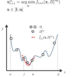
surrogate models. As a result, the samples inDtop_t will become concentrated in a local area, which hopefully is within the basin the global optimum. Taking Fig. 2 as an example, the circles denote all samples in Dt and filled circles indicate

the samples inDtop_t . Solutions inD_ttopdistribute in the local area [l,u], which is within the basin of the global optimum. Another local ensemble surrogate modelfˆens(x, Dtopt )based

onDtop_t , denoted by the dotted line in Fig. 2, is built to allow the PSO algorithm to exploit the optimum located in this area. The local search is to find the solution xls_t+1 minimizing the criterion described in Equation (15).

xls_t+1= arg min x ˆ fens(x, Dtopt ) x∈[l,u] (15)

Fig. 2. Illustration of local model management. All circles are samples inDt

and the filled circles are the samples inDtopt . The local modelfˆens(x, Dtopt )

is built within the region[l,u]in the search space.

Once the local optimum is found, it will be evaluated using the expensive objective function and the new data pair

xls t+1, ytls+1

is added toDt.

IV. EXPERIMENTALRESULTS ONBENCHMARKPROBLEMS

In this section, we first present empirical studies that eval-uate the performance of the proposed algorithm with respect to the influence of QBC based model management and local model management, sensitivity analysis of some parameters of the algorithm, and its scalability to the search dimension. Then, we compare CAL-SAPSO with a few state-of-the-art SAEAs on a set of widely used benchmark problems. During the comparison, 20 independent runs are performed for each algorithm.

All surrogate models used in this work and compared algorithms are implemented using the SURROGATES toolbox [49], which is based on two other toolboxes including DACE [50] and RBF [51]. The details of training the three models are given below.

• PR: the least-squares regression is used for training.

• RBF: the gradient descent method is adopted for learning the centers, weights, and spreads.

• Kriging: the Hooke & Jeeves method [52] that is an ef-ficient coordinate search is employed for hyperparameter optimization.

A. Behavior Study of CAL-SAPSO

To study the influence of each major component of the proposed algorithm on the its performance, we conducted various experiments on the modified Rastrigin problem with adjustable parameters in Equation (16), which has ld local optima with a height of h. Thus, the modified Rastrigin problem becomes uni-modal whenl equals 1.

fModified Rastrigin(x) = d P i=1 (x2 i +h(1−cos(lπxi))) x∈[−1,1]d (16)

1) Parameter Sensitivity Analysis: Here, the PSO is initial-ized with 100 random solutions instead of solutions inDtto

avoid getting trapped in local area ofDt. The only parameter

in the PSO is the stopping condition. We test the proposed algorithm using different gmax(20, 50, 100, and 200) on two

modified Rastrigin problems, i.e. (h = 10, l = 1) as a uni-modal and (h = 1, l = 10) as a multi-modal optimization problem. The average best fitness values obtained by CAL-SAPSOs with different gmax are shown in Table I. It is clear

the best performance is achieved when gmax = 100 in both

cases. Therefore, we setgmaxto 100 for CAL-SAPSO in the

following experiments.

TABLE I

AVERAGE BEST FITNESS VALUES(SHOWN ASAVG±STD)OBTAINED BY CAL-SAPSOS WITH DIFFERENTgmaxON THE MODIFIEDRASTRIGIN

PROBLEMS(d= 20).

gmax (h= 10, l= 1) (h= 1, l= 10)

20 4.85e-02±9.81e-03 1.42e+00±1.47e-01 50 1.54e-02±3.82e-03 1.84e-01±5.18e-02 100 1.44e-02±8.15e-03 1.18e-01±5.78e-02

200 5.27e-02±8.49e-03 1.95e-01±4.19e-02

2) Effect of the Global Model Management: To show the role of QBC based model management in CAL-SAPSO, we compare two variants of CAL-SAPSO with and with-out the uncertainty based criterion (denoted as CAL-SAPSO and CAL-SAPSO-WOU) on two modified Rastrigin problems (d = 20), i.e. (h = 10, l = 1) as a uni-modal and (h = 1, l= 10)as a multi-modal optimization problem. In addition, we also compared the QBC based model management with the widely used infill sampling criteria in Kriging-assisted evolutionary optimization, including LCB and ExI. To enable a fair comparison, LCB and ExI use the same settings for the Kriging model and the optimizer, the only difference is that LCB and ExI replace the three infilling criteria by LCB or ExI. The convergence profiles of these four algorithms are plotted in Fig. 3, where the first 100 exact FEs are the initial samples determined by Latin hypercube sampling in the dataset before optimization starts.

From Fig. 3, we can see that both variants of the CAL-SAPSO converge faster than LCB and ExI on both uni-modal and multi-modal test functions. Comparing LCB and ExI, we find that LCB converges slightly faster than ExI on the uni-modal problem, while ExI converges slightly faster than LCB on the multi-modal problem. We also note that the uncertainty based criterion appears to have little influence on the performance on the uni-modal problem, which is expected.

Fig. 3. Convergence profiles of CAL-SAPSO, CAL-SAPSO-WOU, LCB, and ExI on the modified Rastrigin problems (d= 20).

From these result, we can surmise that the uncertainty based criterion is very important for optimization of multi-modal problems.

Furthermore, we compare the above four algorithms on the modified Rastrigin problems (d = 20, h = 1) with various l. Note that the number of local optima of the modified Rastrigin problem increases as l increases. The average best fitness values obtained by these four algorithms are shown in Table II. We conducted Friedman tests with the Bergmann-Hommel post-hoc test [53] to analyze the results presented in Table II and the p-values are shown in Table III. From these results, we can see that CAL-SAPSO significantly outperforms LCB and ExI, while CAL-SAPSO-WOU cannot significantly outperform LCB and ExI. These results demonstrate that the proposed uncertainty-based model management strategy is able improve the performance of CAL-SAPSO.

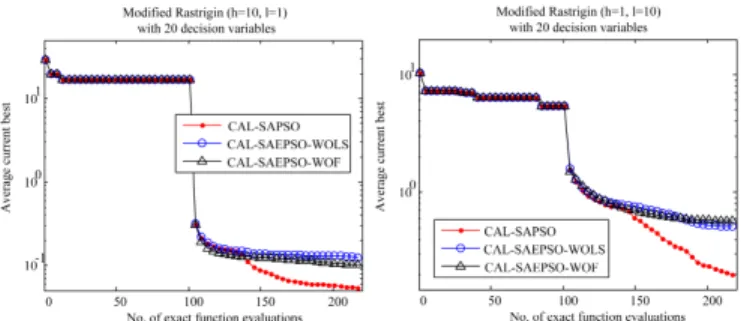
3) Effect of Local Model Management: To demonstrate the effect of the local search based model management, we compare different variants of the CAL-SAPSO on two mod-ified Rastrigin problems (d= 20), i.e., a uni-modal problem when (h = 10, l = 1), and a multi-modal problem when (h= 1, l= 10). In addition to the comparison between CAL-SAPSO variants with and without local search based model management (denoted as CAL-SAPSO and CAL-SAPSO-WOLS), we also compare a CAL-SAPSO variant without using performance based criterion (CAL-SAPSO-WOF) to show the different influence of the performance based criterion within the global QBC based model management and local model management. The convergence profiles of the three compared algorithms are presented in Fig. 4, where the first 100 exact FEs are the initial samples in the dataset.

Fig. 4. Convergence profiles of CAL-SAPSO, CAL-SAPSO-WOLS, and CAL-SAPSO-WOF on the modified Rastrigin problems (d= 20).

TABLE II

AVERAGE BEST FITNESS VALUES(SHOWN ASAVG±STD)OBTAINED BYCAL-SAPSO, CAL-SAPSO-WOU, LCB,ANDEXION THE MODIFIED RASTRIGIN PROBLEMS(d= 20).

l CAL-SAPSO CAL-SAPSO-WOU LCB ExI

1 3.64e-04±3.26e-04 7.85e-03±2.78e-03 3.27e+00±3.76e-01 3.65e+00±2.36e-01 3 5.26e-03±3.18e-03 1.05e-01±3.02e-02 3.78e+00±3.48e-01 4.04e+00±3.00e-01 5 3.30e-04±2.46e-04 4.97e-03±1.12e-03 2.06e+00±6.06e-01 2.64e+00±4.29e-01 10 1.18e-01±5.78e-02 1.16e+00±8.06e-02 4.01e+00±3.54e-01 3.84e+00±3.98e-01

Average rank 1.000 2.000 3.250 3.750

TABLE III

p-VALUES OFFRIEDMAN TEST WITH THEBERGMANN-HOMMEL POST-HOC TEST(SIGNIFICANT LEVEL=0.05)FOR THE COMPARISONS AMONGCAL-SAPSO, CAL-SAPSO-WOU, LCB,ANDEXION THE

MODIFIEDRASTRIGIN PROBLEMS(d= 20). THE SIGNIFICANT DIFFERENCES ARE HIGHLIGHTED. CAL-SAPSOAND CAL-SAPSO-WOUARE NOTATED ASCALANDWOUFOR SIMPLICITY.

CAL WOU LCB ExI

CAL NA 0.273 0.014 0.003

WOU 0.273 NA 0.171 0.055

LCB 0.014 0.171 NA 0.584 ExI 0.003 0.055 0.584 NA

As shown in Fig. 4, the local model management can improve the performance of CAL-SAPSO in particular in the later stage, although the improvement on the uni-modal problem is not as significant as that on the multi-modal problem. For the uni-modal problem, CAL-SAPSO-WOLS and CAL-SAPSO-WOF have a similar performance. For the multi-modal problem, CAL-SAPSO-WOF is slightly worse than CAL-SAPSO-WOLS, probably because local manage-ment only may easily get trapped in a local optimum. These comparative results suggest that it is necessary to use both uncertainty and performance based global model management, and the performance can be further enhanced by introducing an additional local model management process.

To more quantitatively assess the contribution made by the global model management and local model management in CAL-SAPSO, we calculate the percentage of improvements contributed by global and local model management (xf and

xls) in CAL-SAPSO, respectively, on both problems. The results are plotted in Fig. 5, where the contribution is de-fined as the improvement of yf_t+1 or ylst+1 compared to the

previous samples in the dataset Dt. In other words, a range

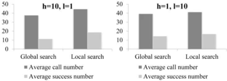
of [0%,100%] contribution percentage can be mapped to the interval between the best sample in the initial dataset and the obtained best solution. From these figures, we can see that the local model management has contributed more than 10% of the overall improvement on the multi-modal test problem, but only less than 1% improvement on the uni-modal problem. Fig. 6 records the average number of global model management (each of which uses two expensive FEs) and the number of successful global and local searches on these two test problems, where a successful search means that a better solution is obtained by applying one global or local search (xf

andxls). For the uni-modal Rastrigin problem, CAL-SAPSO is able to strike a good balance between global and local search, and the success rate of both global and local model management is around 50%, while a slightly low success rate

can be achieved on the multi-modal test problem.

Fig. 5. Percentage of contribution made by the global and local model management on modified Rastrigin problems (d= 20).

Fig. 6. Average number of global and local search versus the number successful global and local searches on modified Rastrigin problems (d= 20).

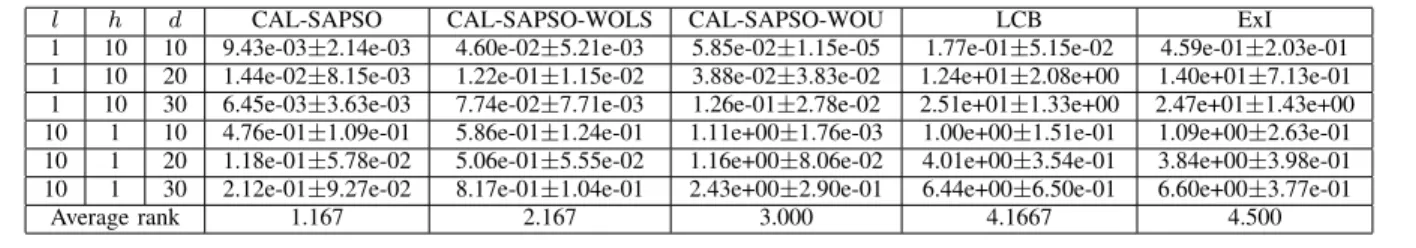
4) Scalability: To examine the scalability of CAL-SAPSO to the dimension of the decision space, we compare three CAL-SAPSO variants (CAL-SAPSO, CAL-SAPSO-WOLS, and CAL-SAPSO-WOU) with LCB and ExI based model management strategies on two modified Rastrigin problems of various numbers of decision variables (d = 10,20,30). Again, the Rastrigin function is a uni-modal function when (h = 10, l = 1), and a multi-modal problem when (h = 1, l = 10). The obtained average best fitness values obtained by these five compared algorithms are listed in Table IV.

We employ the Friedman test with the Bergmann-Hommel post-hoc test [53] to analyze the results in Table IV, and the p-values are shown in Table V. CAL-SAPSO-WOU signifi-cantly outperforms LCB and ExI, whereas CAL-SAPSO and CAL-SAPSO-WOLS significantly outperform LCB and ExI. The uncertainty-based model management is able to improve the performance of CAL-SAPSO. Comparing CAL-SAPSO with CAL-SAPSO-WOLS, CAL-SAPSO significantly out-performs CAL-SAPSO-WOU, whereas CAL-SAPSO-WOLS cannot significantly outperform CAL-SAPSO-WOU. The local model management strategy slightly improves the performance of SAPSO. We also find that the performance of CAL-SAPSO and CAL-CAL-SAPSO-WOLS is not strongly affected as the dimension of the decision space increases. Note that the

TABLE IV

AVERAGE BEST FITNESS VALUES(SHOWN ASAVG±STD)OBTAINED FROMCAL-SAPSO, CAL-SAPSO-WOLS, CAL-SAPSO-WOU, LCB,ANDEXI ON THE MODIFIEDRASTRIGIN PROBLEMS WITH VARIOUSd.

l h d CAL-SAPSO CAL-SAPSO-WOLS CAL-SAPSO-WOU LCB ExI

1 10 10 9.43e-03±2.14e-03 4.60e-02±5.21e-03 5.85e-02±1.15e-05 1.77e-01±5.15e-02 4.59e-01±2.03e-01 1 10 20 1.44e-02±8.15e-03 1.22e-01±1.15e-02 3.88e-02±3.83e-02 1.24e+01±2.08e+00 1.40e+01±7.13e-01 1 10 30 6.45e-03±3.63e-03 7.74e-02±7.71e-03 1.26e-01±2.78e-02 2.51e+01±1.33e+00 2.47e+01±1.43e+00 10 1 10 4.76e-01±1.09e-01 5.86e-01±1.24e-01 1.11e+00±1.76e-03 1.00e+00±1.51e-01 1.09e+00±2.63e-01 10 1 20 1.18e-01±5.78e-02 5.06e-01±5.55e-02 1.16e+00±8.06e-02 4.01e+00±3.54e-01 3.84e+00±3.98e-01 10 1 30 2.12e-01±9.27e-02 8.17e-01±1.04e-01 2.43e+00±2.90e-01 6.44e+00±6.50e-01 6.60e+00±3.77e-01

Average rank 1.167 2.167 3.000 4.1667 4.500

TABLE V

p-VALUES OFFRIEDMAN TEST WITH THEBERGMANN-HOMMEL POST-HOC TEST(SIGNIFICANT LEVEL=0.05)FOR THE COMPARISONS OF

CAL-SAPSO, CAL-SAPSO-WOLS, CAL-SAPSO-WOU, LCB,AND EXION THE MODIFIEDRASTRIGIN PROBLEMS(d= 20). THE SIGNIFICANT DIFFERENCES ARE HIGHLIGHTED. CAL-SAPSO, CAL-SAPSO-WOLS,ANDCAL-SAPSO-WOUIS SHORTED TOCAL,

WOLS,ANDWOU.

CAL WOLS WOU LCB ExI

CAL NA 0.273 0.045 0.001 0.000

WOLS 0.273 NA 0.361 0.029 0.011

WOU 0.045 0.361 NA 0.201 0.100 LCB 0.001 0.029 0.201 NA 0.715 ExI 0.000 0.011 0.100 0.715 NA

local model management strategy has consistently improved the performance.

In summary, CAL-SAPSO performs well on both uni-modal and multi-uni-modal problems when the number of decision variables changes from 10 to 30.

B. Comparative Experiment on Benchmark Problems To further examine the performance of the proposed algo-rithm, we compare CAL-SAPSO with four popular SAEAs on benchmark problems of different dimensions d = 10,20,30 listed in Table VI. The compared algorithms include GPEME [11], WTA1 [47], GS-SOMA [33], and MAES-ExI (Meta-model assisted EA with ExI as the infill sampling criterion) [26]. To be fair, all settings for the surrogate models (i.e. PR, RBF, and Kriging models) of the compared algorithms are the same as those in CAL-SAPSO. The main characteristics of the four SAEAs to be compared are shown below.

• GPEME: a Kriging-based SAEA with LCB as its criterion for selecting solutions for evaluation tested on median scale problems.

• WTA1: an ensemble-based SAEA with weights assign-ment by the RMSE of PR, RBF, and Kriging models. In the experiment, WTA1 keeps evaluating the optimum of the surrogate ensemble and adds it to the dataset for model updating.

• GS-SOMA: an SAEA using a PR models and a ensemble

model (PR, RBF, and Kriging models).

• MAES-ExI: a Kriging-based SAEA with ExI as its

cri-terion for selecting solutions for evaluation.

All algorithms under comparison begin with 5d exact FEs and terminate after11dexact FEs are exhausted. The average best fitness values obtained by the five algorithms over 20

TABLE VI TEST PROBLEMS.

Problem d Optimum Note

Ellipsoid 10,20,30 0 Uni-modal

Rosenbrock 10,20,30 0 Multi-modal with narrow valley

Ackley 10,20,30 0 Multi-modal

Griewank 10,20,30 0 Multi-modal

Rastrigin 10,20,30 0 Very complicated multi-modal

independent runs are shown in Table VII, and the convergence profiles of the algorithms are plotted in Figs. 7-11.The results in Table VII are analyzed using the Friedman test and thep -values are adjusted according to the Hommel procedure [53], where CAL-SAPSO is the control method. In general, CAL-SAPSO significantly outperforms GPEME and MAES-ExI, which has a better average rank than GS-SOMA and WTA1. The Ellipsoid problem is a uni-modal problem, and the convergence profiles of CAL-SAPSO, GPEME, WTA1, GS-SOMA, and MAES-ExI on the Ellipsoid function of dimen-sionsd= 10,20,30are shown in Fig. 7. All ensemble-based algorithms, CAL-SAPSO, WTA1, and GS-SOMA, are able to find a much better solution, and CAL-SAPSO performs the best ford= 20,30, while GS-SOMA achieves the best result ford= 10. Note that GA-SOMA also uses a global and a local surrogates. By contrast, GPEME and MAES-ExI fail to make sufficient progress, in particular for d= 20,30. These results indicate that uncertainty based model management is helpful also for uni-modal optimization problems, which is consistent with the findings reported in [33].

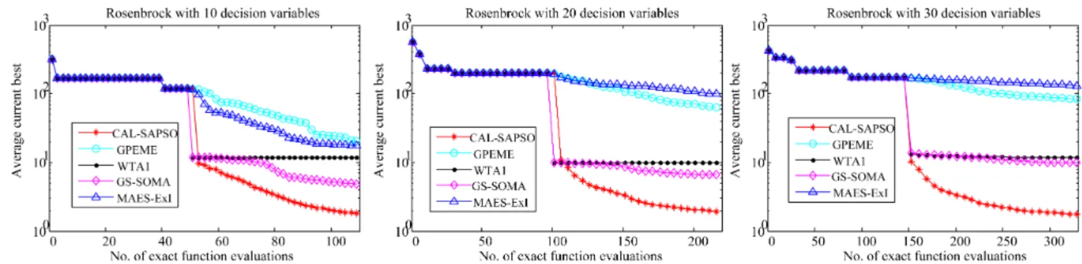
The convergence profiles of CAL-SAPSO, GPEME, WTA1, GS-SOMA, and MAES-ExI on the Rosenbrock function of dimensions d = 10,20,30 are shown in Fig. 8. The Rosen-brock function is a multi-modal problem with a narrow valley leading to the global optimum. Again, the ensemble-based SAEAs, WTA1, GS-SOMA, and CAL-SAPSO outperform GPEME and MAES-ExI. Among the three ensemble based approaches, CAL-SAPSO is able to perform consistently well for d= 10,20,30. GS-SOMA performs better than the plain ensemble method WTA1, but the improvement becomes minor when dimension of the decision space dincreases.

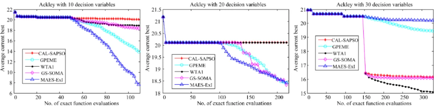
The Ackley function is a multi-modal optimization problem with a very narrow basin around the global optimum. The peak of becomes even more narrower when the dimension d increases. The convergence profiles of the five compared al-gorithms on the Ackley function of dimensionsd= 10,20,30 are shown in Fig. 9. Different to the convergence profiles on

TABLE VII

AVERAGE BEST FITNESS VALUES(SHOWN ASAVG±STD)OBTAINED BYCAL-SAPSO, GPEME, WTA1, GS-SOMA,ANDMAES-EXI,WHICH ARE ANALYZED BY THEFRIEDMAN TEST. THEp-VALUES ARE ADJUSTED BY THEHOMMEL PROCEDURE(CAL-SAPSOIS THE CONTROL METHOD,THE

SIGNIFICANT LEVEL IS0.05).

Problem d CAL-SAPSO GPEME WTA1 GS-SOMA MAES-ExI

Ellipsoid 10 8.79e-01±8.51e-01 3.78e+01±1.53e+01 3.00e+00±2.02e-03 1.77e-01±1.65e-01 1.74e+01±7.36e+00 Ellipsoid 20 1.58e+00±4.83e-01 3.19e+02±9.03e+01 2.17e+01±8.51e+00 9.97e+00±3.41e+00 5.22e+02±5.58e+01 Ellipsoid 30 4.02e+00±1.08e+00 1.23e+03±2.24e+02 8.56e+01±1.17e+01 6.67e+01±1.11e+01 1.71e+03±1.77e+02 Rosenbrock 10 1.77e+00±3.80e-01 2.07e+01±7.44e+00 1.18e+01±2.13e-03 4.77e+00±1.14e+00 1.69e+01±4.63e+00 Rosenbrock 20 1.89e+00±3.32e-01 6.15e+01±2.19e+01 1.00e+01±3.90e-02 6.52e+00±1.13e+00 9.81e+01±2.42e+01 Rosenbrock 30 1.76e+00±3.96e-01 8.42e+01±2.79e+01 1.18e+01±8.19e-01 9.82e+00±1.10e+00 1.32e+02±1.66e+01 Ackley 10 2.01e+01±2.44e-01 1.38e+01±2.50e+00 1.90e+01±1.23e+00 1.84e+01±1.73e+00 7.49e+00±3.77e+00

Ackley 20 2.01e+01±0.00e+00 1.84e+01±9.19e-01 2.01e+01±0.00e+00 1.83e+01±1.99e+00 1.84e+01±1.30e+00 Ackley 30 1.62e+01±4.13e-01 1.95e+01±4.39e-01 1.51e+01±6.98e-01 1.61e+01±3.61e-01 2.02e+01±1.30e-01 Griewank 10 1.12e+00±1.21e-01 2.72e+01±1.13e+01 1.07e+00±2.04e-02 1.08e+00±1.78e-01 1.20e+01±5.19e+00 Griewank 20 1.06e+00±3.66e-02 1.37e+02±3.21e+01 2.00e+00±4.32e-01 1.17e+00±6.37e-02 2.64e+02±1.54e+01 Griewank 30 9.95e-01±3.99e-02 2.84e+02±5.25e+01 3.22e+00±3.25e-01 2.51e+00±4.06e-01 4.47e+02±3.14e+01 Rastrigin 10 8.88e+01±2.26e+01 7.15e+01±1.27e+01 9.58e+01±3.20e+00 1.05e+02±1.52e+01 8.75e+01±1.29e+01 Rastrigin 20 7.51e+01±1.44e+01 1.69e+02±2.86e+01 1.53e+02±3.12e+00 1.54e+02±4.23e+00 1.91e+02±1.91e+01 Rastrigin 30 8.78e+01±1.65e+01 2.86e+02±3.06e+01 2.54e+02±3.07e+01 2.81e+02±2.66e+01 3.70e+02±2.16e+01

Average rank 1.967 3.733 2.833 2.267 4.200

Adjustedp-value NA 0.007 0.267 0.603 0.000

Fig. 7. Convergence profiles of CAL-SAPSO, GPEME, WTA1, GS-SOMA, and MAES-ExI on the Ellipsoid function of dimensionsd= 10,20,30.

Fig. 8. Convergence profiles of CAL-SAPSO, GPEME, WTA1, GS-SOMA, and MAES-ExI on the Rosenbrock function of dimensionsd= 10,20,30.

the Ellipsoid and Rosenbrock functions, the ensemble based methods are outperformed by GPEME and MAES-ExI on the 10-dimensional Ackley function, although they are not able to perform well on 20- and 30-dimensional Ackley functions. We can observe that on the Ackley function, none of the compared algorithm can perform consistently well. This might be due to the narrow peak around the optimum, which makes it very difficult for the surrogate to effectively learn the fitness landscape.

The convergence curves of the compared algorithm on the multi-modal Griewank function of dimensions d= 10,20,30

are shown in Fig. 10. From the figure, we can observe that the three ensemble based methods CAL-SAPSO, WTA1 and GS-SOMA perform similarly well, and all better than GPEME and MAES-ExI. Among the three ensemble based methods, CAL-SAPSO outperforms GS-SOMA and WTA1 on the 30-dimensional Griewank function.

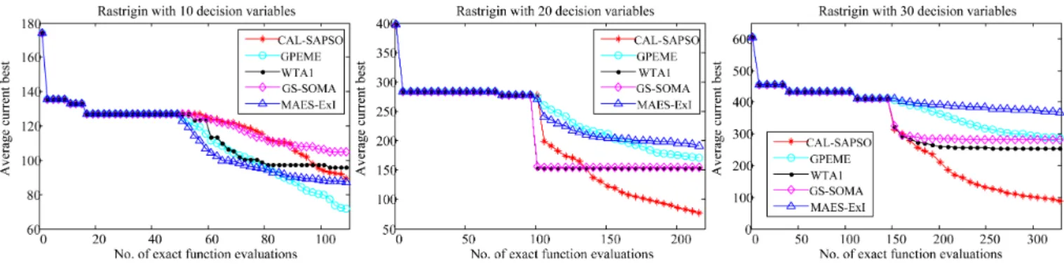
Finally, we examine the performance of the algorithms on the multi-modal Rastrigin function. The convergence curves of all the compared algorithm on the Rastrigin function of dimensions d = 10,20,30 are plotted in Fig. 11. While all the compared algorithms perform comparatively on the

10-Fig. 9. Convergence profiles of CAL-SAPSO, GPEME, WTA1, GS-SOMA, and MAES-ExI on the Ackley function of dimensionsd= 10,20,30.

Fig. 10. Convergence profiles of CAL-SAPSO, GPEME, WTA1, GS-SOMA, and MAES-ExI on the Griewank functions of dimensionsd= 10,20,30

dimensional Rastrigin function, CAL-SAPSO performs the best on the 20- and 30-dimensional Rastrigin functions.

From the above results, we can see that CAL-SAPSO performs the best in eight out of the ten instances on the five test problems of dimensions 20 and 30 when the computation budget is limited to 220 and 330 FEs, respectively. Note how-ever that the performance of CAL-SAPSO is less competitive on 10-dimensional test functions, probably because the number of expensive FEs is too small, as only 60 new solutions are evaluated during the optimization. Of these 60 newly evaluated solutions, almost half of them are consumed in the uncertainty-based model management, leaving little opportunity for CAL-SAPSO to sufficiently exploit the search space.

However, CAL-SAPSO, like all other SAEAs examined in this work, has performed poorly on the Ackley function. The bad performance of the SAEAs on the Ackley function might be attributed to the very narrow and deep peak of the fitness landscape round the global optimum and the large number of local optima, causing major difficulties for the surrogate to learn sufficient information about the landscape around the global optimum with a very limited number of training samples.

Another observation we can make is that CAL-SAPSO, GS-SOMA and WTA1, all of which use a heterogeneous ensemble, perform more robustly on various problems compared to GPEME and MAES-ExI, which use one single model as the surrogate. This observation suggests that an heterogeneous ensemble is more reliable for fitness estimation when little is known about the problem to be optimized.

It appears that a maximum of 11d FEs is inadequate for

exploring all local optima for the above benchmark problems. To further examine the performance of the ensemble- and non-ensemble-based algorithms, we increased the allowed compu-tational budget to 1000 FEs and compare the performance of CAL-SAPSO (ensemble-based) and GPEME (non-ensemble-based) on 30-dimensional Ackley and Rastrigin functions. Their convergence curves are shown in Fig. 12. On the Ackley functions, CAL-SAPSO outperforms GPEME at the begin-ning. However, CAL-SAPSO gets trapped in local optima, while the solution found by GPEME keeps improving and GPEME outperforms CAL-SAPSO after 800 FEs. For the Rastrigin function, CAL-SAPSO outperforms GPEME during the 1000 FEs. These results indicate that the performance of CAL-SAPSO will become less superior to that of GPEME when more FEs are allowed.

Note that Kriging models are mainly suited for low-dimensional problems (typically less than 15) due to its prohibitively high computational complexity as the dimension of the problem becomes high [18]. It is known that the compu-tational complexity of constructing a Kriging model isO(n3₎

[18], [54], where nis the size of training data. As shown in [11], building a Kriging model using 150 training data for a 50-dimensional problem with the MATLAB optimization toolbox optimizing hyperparameters takes from 240 to 400 seconds, which means that it may take from 1000 to 1800 seconds and from 12000 to 20000 seconds, when the number of training data is 250 (5d) and 550 (11d), respectively, for 50-dimensional problems. Obviously, using kriging models as computationally efficient surrogates no longer makes sense for high-dimensional problems. Even if the MATLAB

optimiza-Fig. 11. Convergence profiles of CAL-SAPSO, GPEME, WTA1, GS-SOMA, and MAES-ExI on the Rastrigin function of dimensionsd= 10,20,30.

Fig. 12. Convergence profiles of CAL-SAPSO and GPEME on the 30-dimensional Ackley and Rastrigin functions.

tion toolbox is replaced by the computationly more efficient Hooke & Jeeves method [52], building a Kriging moddel still takes 10 and 100 seconds when the number of training data is 250 and 550, respectively, as shown in [54]. Thus, constructing a Kriging model itself becomes a computationally expensive problem as the training data increases, no matter which optimizer is used for optimizing its hyperparameters. Worse, although optimizing the hyperparameters of the Kriging model using the Hooke & Jeeves method [52] is able to significantly reduce the computation time, the performance of the Kriging model degenerates considerably. For example, the optimal solution obtained by GPEME on the 30-dimensional Ackley function reported in [11] is 5, while the result obtained in this work degrades to 13 when the hyperparameters of the Kriging model is optimized using the Hooke & Jeeves method. We also compare CAL-SAPSO with GPEME without dimension reduction on the 50-dimensional Rastrigin function and the convergence profiles are presented in Fig. 13. From the figure, we can see that CAL-SAPSO outperforms GPEME.

To further compare the algorithms based on different methodologies, we test CAL-SAPSO and GPEME on four 30-dimensional multi-modal CEC’ 05 test problems [55], which are F6 (shifted Rosenbrock’s Function), F7 (shifted rotated Griewank’s Function), F8 (shifted rotated Ackley’s Function), and F10 (shifted rotated Rastrigin’s Function), which are harder than the problems tested in Table VII. Note that we remove the constant fbias from those four test problems so

that the optimum lies on the origin. Table VIII lists the average best fitness values obtained by CAL-SAPSO and GPEME on F6, F7, F8, and F10, from we can see that CAL-SAPSO outperforms GPEME on all problems.

Fig. 13. Convergence profiles of CAL-SAPSO and GPEME on the 50-dimensional Rastrigin function.

TABLE VIII

AVERAGE BEST FITNESS VALUES(SHOWN ASAVG±STD)OBTAINED BY CAL-SAPSOANDGPEMEON30-DIMENSIONALCEC’ 05TEST PROBLEMS(F6, F7, F8,ANDF10). THEWILCOXON SIGNED-RANK TEST

CONDUCTED FOR STATISTICAL SIGNIFICANCE AT A SIGNIFICANT LEVEL=0.05.

Problem CAL-SAPSO GPEME p-value

F6 1.38e+03±2.12e+03 1.18e+04±3.88e+03 1.03e-04 F7 1.00e+00±2.09e-02 2.83e+02±5.36e+01 8.86e-05 F8 1.64e+01±5.98e-01 1.93e+01±7.40e-01 8.86e-05 F10 2.49e+02±2.44e+01 3.77e+02±4.12e+01 8.86e-05

V. AIRFOILDESIGN

To examine the performance of CAL-SAPSO on real-world problems, we present here the simulation results of CAL-SAPSO applied to a transonic airfoil design optimization prob-lem. Predicting airfoil performance requires time-consuming CFD simulations, leading to a computationally expensive optimization problem. In the following, we first present a very brief formulation of the problem and then the comparative results.

A. Problem Formulation

The airfoil design problem adopted in this work is based on the RAE2822 airfoil test case described within the GARTEUR AG52 project. The target of the design is to optimize the geometry of the airfoil defined by 14 controlling points of a non-rational B-spline (NURBS) to minimize the drag over lift

ratio at two different transonic conditions as shown in Equation (17):

fAirf oil= min

2 X i=1 wi( Cd Cl _Cb d Cb l ) i , (17)

where, for each flight design condition i, Cd and Cl are the

drag and lift coefficients, respectively, for the designed airfoil, C_db andC_lb are the drag and lift coefficients for the baseline airfoil, andwiis the weight assigned to each design condition

(each set to 0.5 in the current study). Hence the objective fAirf oil= 1for the baseline RAE2822 airfoil. An expensive

CFD simulation is required to calculate Cd and Cl for each

transonic condition for any given geometry. A full description of the test case is available from the GARTEUR AG52 project website1_.

B. Results

CAL-SAPSO, as well as other three SAEAs, including WTA1, GPEME, and GS-SOMA are employed to optimize the geometry of the RAE2822 airfoil. As both MAES-ExI and GPEME employ Kriging based infill sampling criteria, and they have similar performance on benchmark problems in Section IV-B, we exclude MAES-ExI in this section. All the algorithms start with 5dinitial sample and terminates by 11d exact function evaluations, and each algorithm is run 20 times, and their average best fitness values are given in Table IX. From these results, we can confirm that CAL-SAPSO outperforms other compared algorithms.

TABLE IX

AVERAGE BEST FITNESS VALUES OBTAINED BYCAL-SAPSO, WTA1, GPEME,ANDGS-SOMAON THERAE2822AIRFOIL TEST CASE. THE

BEST RESULTS ARE HIGHLIGHTED.

Algorithm Avg Std

Baseline RAE2822 1.00e-00 NA CAL-SAPSO 6.84e-01 1.08e-02

WTA1 7.79e-01 1.06e-02 GPEME 7.78e-01 9.99e-03 GS-SOMA 7.44e-01 2.18e-02

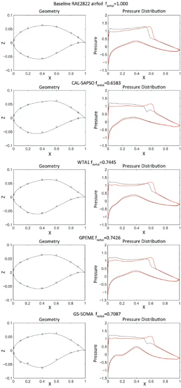
The four best designs obtained by the compared algorithms, together with the baseline RAE2822 airfoil, are shown in Fig. 14. The left panel in each sub-figure of Fig. 14 describes the geometry of the obtained optimal design, where the plus signs indicate the 14 NURBS control points. The right panel in each sub-figure of Fig. 14 shows the distribution of local pressure coefficient over the upper and lower surfaces of the airfoil design, for each of the two transonic flight conditions. For the baseline RAE2822 airfoil, Fig. 14 shows a rapid change in the pressure coefficient on the airfoil upper surface near X=0.6 for both flight conditions. This highlights the presence of shock waves, which in turn will lead to a high drag coefficient. For transonic flows, the location and strength of shock waves are extremely sensitive to very small changes in the overall airfoil shape. For each of the designed airfoils, it can be seen that the strength of these shock wave features have been reduced by varying amounts, leading to an improvement in the objective

1_{http://www.garteur.org/}

function for all the algorithms. The designs from CAL-SAPSO and GS-SOMA show similar pressure distributions, with CAL-SAPSO achieving the lowest overall level of the objective.

Fig. 14. The baseline design and the best designs obtained by CAL-SAPSO, WTA1, GPEME, and GS-SOMA.

VI. CONCLUSION

This paper proposes an ensemble-based model management strategy combining uncertainty and performance based criteria for surrogate-assisted evolutionary optimization of computa-tionally expensive problems. The basic idea is inspired by QBC in active learning that selects the sample having the

largest degree of uncertainty among the committee members. In addition to the QBC based global model management, a local model management strategy is also proposed to enhance local search ability. The ensemble surrogate in this work is composed of three types of models, one PR model, one RBF model and one Kriging model, making the performance more robust to various optimization problems. The proposed algorithm is examined on uni-modal and multi-modal test problems of dimensions of 10, 20, 30, and 50. Simulation results demonstrate that the proposed algorithm outperforms four state-of-the-art SAEAs compared in this work on the ma-jority of the 20- and 30-dimensional test problems for a limited computation budget. The superiority of the performance of the proposed algorithm is confirmed on an 14-dimensional airfoil design optimization problem.

Despite the promising performance of the proposed algo-rithm on the 20- and 30-dimensional test problems considered in this work, its performance on 10-dimensional problems is less competitive, where the computational budget is particu-larly small. One reason might be that most expensive fitness evaluations done online are exhausted in the uncertainty-based model management stage and the algorithm is not able to adequately exploit the search space. Thus, our future work is to adaptively allocate the available resources to the three model management stages so that the limited budget can be fully taken advantage of. In addition, the proposed algorithm has been examined on optimization problems up to a dimension of 50. In the future, we will also extend the proposed algorithm to deal with higher dimensional expensive optimization problems.

In the proposed algorithm, PSO is adopted as the optimizer. It should be mentioned that other metaheuristic optimization algorithms such as evolution strategies can replace the PSO. Thus, it is of interest to empirically compare the performance of the proposed algorithm when a different metaheuristic algorithm is adopted as the optimizer.

REFERENCES

[1] P. J. Fleming and R. C. Purshouse, “Evolutionary algorithms in control systems engineering: a survey,”Control engineering practice, vol. 10, no. 11, pp. 1223–1241, 2002.

[2] J. Knowles, “ParEGO: a hybrid algorithm with on-line landscape ap-proximation for expensive multiobjective optimization problems,”IEEE Transactions on Evolutionary Computation, vol. 10, no. 1, pp. 50–66, 2006.

[3] D. Lim, Y.-S. Ong, Y. Jin, and B. Sendhoff, “Evolutionary optimization with dynamic fidelity computational models,” inInternational Confer-ence on Intelligent Computing. Springer, 2008, pp. 235–242. [4] A. I. Forrester, A. S´obester, and A. J. Keane, “Multi-fidelity optimization

via surrogate modelling,” inProceedings of the royal society of london a: mathematical, physical and engineering sciences, vol. 463, no. 2088. The Royal Society, 2007, pp. 3251–3269.

[5] Y. Jin, “Surrogate-assisted evolutionary computation: Recent advances and future challenges,”Swarm and Evolutionary Computation, vol. 1, no. 2, pp. 61–70, 2011.

[6] B. Liu, S. Koziel, and Q. Zhang, “A multi-fidelity surrogate-model-assisted evolutionary algorithm for computationally expensive optimiza-tion problems,”Journal of Computational Science, vol. 12, pp. 28–37, 2016.

[7] Y. Jin and B. Sendhoff, “A systems approach to evolutionary multiob-jective structural optimization and beyond,”Computational Intelligence Magazine, IEEE, vol. 4, no. 3, pp. 62–76, 2009.

[8] Y. Jin, “A comprehensive survey of fitness approximation in evolutionary computation,”Soft Computing, vol. 9, no. 1, pp. 3–12, 2005.

[9] Y. Jin, M. Olhofer, and B. Sendhoff, “A framework for evolutionary optimization with approximate fitness functions,”IEEE Transactions on Evolutionary Computation, vol. 6, no. 5, pp. 481–494, 2002.

[10] H. Wang, Y. Jin, and J. O. Jansen, “Data-driven surrogate-assisted multiobjective evolutionary optimization of a trauma system,” IEEE Transactions on Evolutionary Computation, vol. 20, no. 6, pp. 939–952, 2016.

[11] B. Liu, Q. Zhang, and G. G. Gielen, “A Gaussian process surrogate model assisted evolutionary algorithm for medium scale expensive opti-mization problems,” IEEE Transactions on Evolutionary Computation, vol. 18, no. 2, pp. 180–192, 2014.

[12] Y. Jin and B. Sendhoff, “Reducing fitness evaluations using clustering techniques and neural network ensembles,” inProceedings of the 6th An-nual Conference on Genetic and Evolutionary Computation. Springer, 2004, pp. 688–699.

[13] D. Lim, Y.-S. Ong, Y. Jin, and B. Sendhoff, “A study on metamodeling techniques, ensembles, and multi-surrogates in evolutionary computa-tion,” in Proceedings of the 9th Annual Conference on Genetic and Evolutionary Computation. ACM, 2007, pp. 1288–1295.

[14] Z. Zhou, Y. S. Ong, M. H. Nguyen, and D. Lim, “A study on polynomial regression and Gaussian process global surrogate model in hierarchical surrogate-assisted evolutionary algorithm,” inEvolutionary Computation, 2005. CEC 2005. IEEE Congress on, vol. 3. IEEE, 2005, pp. 2832–2839.

[15] I. Loshchilov, M. Schoenauer, and M. Sebag, “Comparison-based opti-mizers need comparison-based surrogates,” inParallel Problem Solving from Nature, PPSN XI. Springer, 2010, pp. 364–373.

[16] R. G. Regis, “Evolutionary programming for high-dimensional con-strained expensive black-box optimization using radial basis functions,”

IEEE Transactions on Evolutionary Computation, vol. 18, no. 3, pp. 326–347, 2014.

[17] C. Sun, Y. Jin, J. Zeng, and Y. Yu, “A two-layer surrogate-assisted particle swarm optimization algorithm,”Soft Computing, vol. 19, no. 6, pp. 1461–1475, 2015.

[18] T. Chugh, Y. Jin, K. Miettinen, J. Hakanen, and K. Sindhya, “A surrogate-assisted reference vector guided evolutionary algorithm for computationally expensive many-objective optimization,”IEEE Trans-actions on Evolutionary Computation, vol. PP, no. 99, pp. 1–1, 2016. [19] T. Chugh, N. Chakraborti, K. Sindhya, and Y. Jin, “A data-driven

surrogate-assisted evolutionary algorithm applied to a many-objective blast furnace optimization problem,”Materials and Manufacturing Pro-cesses, vol. PP, pp. 1–29, 2016, doi:10.1080/10426914.2016.1269923. [20] D. Guo, T. Chai, J. Ding, and Y. Jin, “Small data driven evolutionary

multi-objective optimization of fused magnesium furnaces,” in IEEE Symposium Series on Computational Intelligence. Athens, Greece: IEEE, December 2016.

[21] Y. Jin, M. Olhofer, and B. Sendhoff, “On evolutionary optimization with approximate fitness functions,” inProceedings of the 2nd Annual Con-ference on Genetic and Evolutionary Computation. Morgan Kaufmann Publishers Inc., 2000, pp. 786–793.

[22] P. B. Nair, A. J. Keane, and R. Shimpi, “Combining approximation con-cepts with genetic algorithm-based structural optimization procedures,” in Proceedings of the 39th AIAA/ASME/ASCE/AHS/ASC Structures, Structural Dynamics and Materials Conference, 1998, pp. 1741–1751. [23] J. Branke and C. Schmidt, “Faster convergence by means of fitness

estimation,”Soft Computing, vol. 9, no. 1, pp. 13–20, 2005.

[24] M. Emmerich, A. Giotis, M. ¨Ozdemir, T. B¨ack, and K. Giannakoglou, “Metamodel–assisted evolution strategies,” inParallel Problem Solving from Nature–PPSN VII. Springer, 2002, pp. 361–370.

[25] D. R. Jones, M. Schonlau, and W. J. Welch, “Efficient global optimiza-tion of expensive black-box funcoptimiza-tions,”Journal of Global optimization, vol. 13, no. 4, pp. 455–492, 1998.

[26] M. T. Emmerich, K. C. Giannakoglou, and B. Naujoks, “Single-and multiobjective evolutionary optimization assisted by gaussian random field metamodels,” IEEE Transactions on Evolutionary Computation, vol. 10, no. 4, pp. 421–439, 2006.

[27] Z. Zhou, Y. S. Ong, P. B. Nair, A. J. Keane, and K. Y. Lum, “Combining global and local surrogate models to accelerate evolutionary optimiza-tion,” IEEE Transactions on Systems, Man, and Cybernetics, Part C: Applications and Reviews, vol. 37, no. 1, pp. 66–76, 2007.

[28] W. Ponweiser, T. Wagner, and M. Vincze, “Clustered multiple gen-eralized expected improvement: A novel infill sampling criterion for surrogate models,” inEvolutionary Computation, 2008. CEC 2008. IEEE Congress on. IEEE, 2008, pp. 3515–3522.

[29] C. Sun, J. Ding, J. Zeng, and Y. Jin, “A fitness approximation assisted competitive swarm optimizer for large scale expensive optimization

problems,” Memetic Computing, vol. PP, no. 99, pp. 1–12, 2016, doi:10.1007/s12293-016-0199-9.

[30] C. Sun, Y. Jin, R. Cheng, J. Ding, and J. Zeng, “Surrogate-assisted co-operative swarm optimization of high-dimensional expensive problems,”

IEEE Transactions on Evolutionary Computation, vol. PP, no. 99, pp. 1–1, 2017, doi: 10.1109/TEVC.2017.2675628.

[31] S. Bagheri, W. Konen, C. Foussette, P. Krause, T. B¨ack, and P. Koch, “SACOBRA: Self-adjusting constrained black-box optimization with RBF,” inProc. 25. Workshop Computational Intelligence, F. Hoffmann and E. H¨ullermeier, Eds. Universit¨atsverlag Karlsruhe, 2015, pp. 87–96. [32] P. Koch, S. Bagheri, W. Konen, C. Foussette, P. Krause, and T. B¨ack, “A new repair method for constrained optimization,” inin Proceedings of the 17th Annual Conference on Genetic and Evolutionary Computation. ACM, 2015, pp. 273–280.

[33] D. Lim, Y. Jin, Y.-S. Ong, and B. Sendhoff, “Generalizing surrogate-assisted evolutionary computation,”IEEE Transactions on Evolutionary Computation, vol. 14, no. 3, pp. 329–355, 2010.

[34] S. Tong, “Active learning: theory and applications,” Ph.D. dissertation, Citeseer, 2001.

[35] R. Burbidge, J. J. Rowland, and R. D. King, “Active learning for re-gression based on query by committee,” inIntelligent Data Engineering and Automated Learning-IDEAL 2007. Springer, 2007, pp. 209–218. [36] A. Chatterjee and P. Siarry, “Nonlinear inertia weight variation for

dynamic adaptation in particle swarm optimization,” Computers & Operations Research, vol. 33, no. 3, pp. 859 – 871, 2006.

[37] B. Settles, “Active learning,”Synthesis Lectures on Artificial Intelligence and Machine Learning, vol. 6, no. 1, pp. 1–114, 2012.

[38] H. S. Seung, M. Opper, and H. Sompolinsky, “Query by committee,” inProceedings of the fifth annual workshop on Computational learning theory. ACM, 1992, pp. 287–294.

[39] P. Melville and R. J. Mooney, “Diverse ensembles for active learning,” inProceedings of the twenty-first international conference on Machine learning. ACM, 2004, p. 74.

[40] Y. Shi and R. Eberhart, “A modified particle swarm optimizer,” in

Evolutionary Computation, 1998. CEC 1998. IEEE Congress on, 1998, pp. 69–73.

[41] M. Parno, T. Hemker, and K. Fowler, “Applicability of surrogates to improve efficiency of particle swarm optimization for simulation-based problems,”Engineering optimization, vol. 44, no. 5, pp. 521–535, 2012. [42] R. G. Regis, “Particle swarm with radial basis function surrogates for expensive black-box optimization,”Journal of Computational Science, vol. 5, no. 1, pp. 12–23, 2014.

[43] C. Praveen and R. Duvigneau, “Low cost PSO using metamodels and inexact pre-evaluation: Application to aerodynamic shape design,”

Computer Methods in Applied Mechanics and Engineering, vol. 198, no. 9, pp. 1087–1096, 2009.

[44] M. Stein, “Large sample properties of simulations using latin hypercube sampling,”Technometrics, vol. 29, no. 2, pp. 143–151, 1987. [45] R. C. Eberhart and Y. Shi, “Comparing inertia weights and constriction

factors in particle swarm optimization,” inEvolutionary Computation, 2000. CEC 2000. IEEE Congress on, vol. 1. IEEE, 2000, pp. 84–88. [46] R. A. Olea, “Geostatistics for engineers and earth scientists,”

Techno-metrics, vol. 42, no. 4, pp. 444–445, 2000.

[47] T. Goel, R. T. Haftka, W. Shyy, and N. V. Queipo, “Ensemble of surrogates,” Structural and Multidisciplinary Optimization, vol. 33, no. 3, pp. 199–216, 2007.

[48] H. Wang, Y. Jin, and X. Yao, “Diversity assessment in many-objective optimization,”IEEE Transactions on Cybernetics, vol. PP, no. 99, pp. 1–1, 2016, doi=10.1109/TCYB.2016.2550502.

[49] F. Viana and T. Goel, “Surrogates toolbox user’s guide,” http://fchegury. googlepages. com,[retrieved Dec. 2009], Tech. Rep., 2010.

[50] S. Lophaven, H. Nielsen, and J. Sondergaard, “Dace: A matlab kriging toolbox. 2002,” Technical University of Denmark, Tech. Rep., 2002. [51] G. Jekabsons, “RBF: Radial basis function interpolation for

mat-lab/octave,” Riga Technical University, Latvia. version, Tech. Rep., 2009. [52] J. S. Kowalik and M. R. Osborne, “Methods for unconstrained

optimiza-tion problems,” 1968.

[53] J. Derrac, S. Garc´ıa, D. Molina, and F. Herrera, “A practical tutorial on the use of nonparametric statistical tests as a methodology for comparing evolutionary and swarm intelligence algorithms,”Swarm and Evolutionary Computation, vol. 1, no. 1, pp. 3–18, 2011.

[54] S. N. Lophaven, H. B. Nielsen, and J. Søndergaard, “Aspects of the matlab toolbox dace,” Informatics and Mathematical Modelling, Technical University of Denmark, DTU, Tech. Rep., 2002.

[55] P. N. Suganthan, N. Hansen, J. J. Liang, K. Deb, Y.-P. Chen, A. Auger, and S. Tiwari, “Problem definitions and evaluation criteria for the CEC

2005 special session on real-parameter optimization,”KanGAL report, vol. 2005005, p. 2005, 2005.