ISSN: 2341-2356
Instituto
Complutense
de Análisis
Económico
Volatility specifications versus probability
distributions in VaR forecasting
Laura Garcia-Jorcano
Department of Economic Analysis and Finance (Area of Financial Economics) Facultad de Ciencias Jurídicas y Sociales,
Universidad de Castilla-La Mancha, Toledo, Spain
Alfonso Novales
Instituto Complutense de Análisis Económico (ICAE), and
Department of Economic Analysis, Facultad de Ciencias Económicas y Empresariales, Universidad Complutense, Madrid, Spain
Abstract
We provide evidence suggesting that the assumption on the probability distribution for return innovations is more influential for Value at Risk (VaR) performance than the conditional volatility specification. We also show that some recently proposed asymmetric probability distributions and the APARCH and FGARCH volatility specifications beat more standard alternatives for VaR fore- casting, and they should be preferred when estimating tail risk. The flexibility of the free power parameter in conditional volatility in the APARCH and FGARCH models explains their better performance. Indeed, our estimates suggest that for a number of financial assets, the dynamics of volatility should be specified in terms of the conditional standard deviation. We draw our results on VaR forecasting performance from i) a variety of back testing approaches, ii) the Model Confidence Set approach, as well as iii) establishing a ranking among alternative VaR models using a precedence criterion that we introduce in this paper.
Keywords
Value-at-risk, back testing, evaluating forecasts, Precedence, APARCH
model, asymmetric distributions
UNIVERSIDAD COMPLUTENSE
MADRID
Working Paper nº 1926
Volatility specifications versus probability
distributions in VaR forecasting
Laura Garcia-Jorcano∗a, Alfonso Novales†b a
Department of Economic Analysis and Finance (Area of Financial Economics), Facultad de Ciencias Jur´ıdicas y Sociales, Universidad de Castilla-La Mancha, 45071 Toledo, Spain
bInstituto Complutense de An´alisis Econ´omico (ICAE), and Department of Quantitative Economics, Facultad de Ciencias Econ´omicas y Empresariales, Universidad Complutense, Campus de Somosaguas, 28223 Madrid, Spain
E-mail addresses: [email protected] (L. Garcia-Jorcano), [email protected] (A. Novales)
April 2019
Abstract
We provide evidence suggesting that the assumption on the probability distribution for return in-novations is more influential for Value at Risk (VaR) performance than the conditional volatility specification. We also show that some recently proposed asymmetric probability distributions and the APARCH and FGARCH volatility specifications beat more standard alternatives for VaR fore-casting, and they should be preferred when estimating tail risk. The flexibility of the free power parameter in conditional volatility in the APARCH and FGARCH models explains their better performance. Indeed, our estimates suggest that for a number of financial assets, the dynamics of volatility should be specified in terms of the conditional standard deviation. We draw our results on VaR forecasting performance fromi) a variety of backtesting approaches,ii) the Model Confi-dence Set approach, as well asiii) establishing a ranking among alternative VaR models using a
precedencecriterion that we introduce in this paper.
Keywords: Value-at-risk, backtesting, evaluating forecasts, Precedence, APARCH model, asym-metric distributions
∗https://orcid.org/0000-0002-3656-8787
1
Introduction
A traditional discussion in risk measurement analysis has been whether volatility models that incorporate a leverage effect, with negative innovations having a larger impact on volatility than positive innovations of the same size, lead to better Value-at-Risk (VaR) forecasts. A second modeling issue refers to whether asymmetric probability distributions for return innovations lead to an improved VaR model.1 The goal of this paper is to examine the relative importance of the two issues for the efficiency of VaR forecasts. The question is crucial for risk managers, since there are so many potential choices for volatility model and probability distributions that it would be very convenient to establish some priorities in modeling returns for risk estimation. To that end, we have performed an extensive analysis of VaR forecasts in assets of different nature, using symmetric and asymmetric probability distributions for the innovations on volatility models with and without leverage. Even though this issue has been examined in previous work, we consider some volatility specifications and probability distributions that are still relatively new in this literature, which allows us to make some progress in modeling financial returns when forecasting Value at Risk.
We consider three general volatility specifications with leverage, GJR-GARCH, APARCH and FGARCH, with the standard symmetric GARCH model as benchmark. The FGARCH model includes as special cases many other volatility specifications, like the symmetric GARCH, GJR-GARCH and APARCH. It is, in fact, a nested family of GJR-GARCH-type models, thereby allowing for testing how simpler models fit the data. The APARCH and FGARCH models take the power on the conditional standard deviation of the innovations as a free parameter, which provides more flexibility to the dynamics of volatility, allowing for shifts and rotations in the news impact curve. The two types of asymmetry in volatility produced by shifts and rotations are distinct, and they should not be treated as substitutes for each other (Hentschel, 1995). As probability distributions for the innovations we compare the performance of the skewed Student-t distribution and skewed Generalized Error distribution as introduced in Fernandez and Steel (1998), the unbounded John-sonSU distribution (Johnson, 1949), skewed Generalized-t distribution (Theodossiou, 1998) and
Generalized Hyperbolic skew Student-t distribution (Aas and Haff, 2006), with the Normal and symmetric Student-t distributions as benchmark. An interesting feature of our work is the consid-eration of a variety of assets of different nature: stock market indexes, individual stocks, interest rates, commodity prices and exchange rates.
We calculate VaR forecasts following the parametric approach. An AR(1) was estimated for daily returns in all cases. The performance of VaR forecasts is examined through standard tests: the unconditional coverage test of Kupiec (1995), the independence and conditional coverage tests of Christoffersen (1998), and the Dynamic Quantile test of Engle and Manganelli (2004). VaR forecasts are also evaluated through the use of the Asymmetric Linear Tick loss function (AlTick) proposed by Giacomini and Komunjer (2005). The combination of 19 assets, 7 probability dis-tributions, 4 volatility specifications and 4 backtests of VaR leads to an extensive set of results that need to be summarized in a search for some consistent conclusions. One of the contributions of this paper is to follow a diverse strategy to summarize test results in search of robust patterns that might suggest some preferred VaR model specifications. We proceed along several lines: i) comparing the number of realized and expected violations of VaR for the alternative models across
1Along the paper we refer to a VaR forecasting model as a combination of a probability distribution and a volatility specification for return innovations.
the set of assets,ii) comparing thep-values achieved by the different models in the VaR valida-tion tests,iii) applying to the alternative models aprecedencecriterion that we introduce in this paper to rank models according to their VaR forecasting performance, iv) following the Model Confidence Set approach to select the most preferred models.
Our results suggest that the important assumption for VaR performance is that of the prob-ability distribution of the innovations, with the choice of volatility model playing a secondary role. Indeed, validation tests for VaR forecasts yield very similar results for a given probability distribution as we change the volatility model. On the contrary, test results drastically change for a given volatility model when we change the assumption on the probability distribution of the innovations. In fact, the main difference arises when we move from symmetric to asymmetric probability distributions for the innovations, a result consistent with work by Lopez and Walter (2000), Angelidis and Degiannakis (2006), Gerlach et al. (2011), Dendramis et al. (2014), and Braione and Scholtes (2016). The unbounded Johnson distribution, the skew Generalized-t dis-tribution and the skewed Generalized Error disdis-tributions precede other asymmetric disdis-tributions, like the skewed Student-t and the Generalized Hyperbolic skewed Student-t in VaR forecasting. Symmetric distributions come out as being clearly inappropriate. On the volatility side, FGARCH and APARCH volatility specifications precede other alternatives. A relevant implication is that the conditional standard deviation, rather than the conditional variance, should often be used to model the volatility dynamics of financial returns. However, these results do not seem to apply to 10-day VaR forecasting, a discrepancy that should be examined in further research.
The remainder of the paper is organized as follows: in Section 2 we present a review of the literature on the questions we analyze. In Section 3 we describe the volatility models and the probability distributions used in our analysis. In Section 4 we present preliminary statistics for our data set. In Section 5 we report the estimates of the VaR models considered. In Section 6 we provide a description of the statistical tests and the loss function used and we asses VaR performance for the different models. Finally, Section 7 concludes the paper.
2
A review of literature
Among parametric methods for VaR estimation, some authors have analyzed the improvement on VaR estimation provided by volatility models with leverage. Giot and Laurent (2003a) estimated daily VaR for stock indexes using different volatility models. They stated that more complex mod-els like APARCH performed better than RiskMetrics or GARCH specifications (for a comparison of volatility models in VaR estimation see also El Babsiri and Zakoian, 2001). Angelidis et al. (2007) show that volatility models with leverage fare better than symmetric specifications, as they capture more efficiently the characteristics of the underlying series and provide better VaR fore-casts since they perform better in the low probability regions that VaR tries to measure (see also Ane, 2006). Working with a large number of individual stocks and exchange rates, McMillan and Kambouroudis (2009) conclude that the APARCH model should be preferred for more extreme VaR forecasts, while the RiskMetrics model seems to be adequate at more moderate significance levels. In their work, RiskMetrics seems adequate in providing volatility forecasts for most Asian markets; however, the APARCH model is superior in obtaining forecasts for the G7 markets, as well as for other European markets and for the larger Asia markets.2
Given the widespread evidence on the skewness of the distribution of asset returns, analyzing whether the assumption of an asymmetric distribution of return innovations leads to more efficient VaR forecasts is a second methodological issue of interest. Based on the influence of leverage effects on the accuracy of VaR forecasts, Brooks and Persand (2003) concluded that models that do not allow for asymmetries either in the unconditional distribution of returns or in the volatil-ity specification underestimate the true VaR. Giot and Laurent (2003a) used daily data for stock market indexes and individual stocks, showing that models that rely on a symmetric density for return innovations underperform with respect to skewed density models that require modeling both the left and right tails of the distribution of returns. Lee and Su (2015) estimate VaR for eight stock market indexes from Europe and Asia by a parametric GARCH approach as well as by the semi-parametric approach of Hull and White (1998). The only asymmetric distribution they consider, the skewed Generalized-t, is shown to have a better VaR forecasting performance than the Student-t, with the Normal distribution being the last in the ranking, according to the unconditional coverage test of Kupiec and two different loss functions. Corlu et al. (2016) in-vestigate the ability of five alternative probability distributions to represent the behavior of daily equity index returns over the period 1979-2014: the skewed Student-t distribution, the generalized lambda distribution, the Johnson system of distributions, the normal inverse Gaussian distribution, and the g-and-h distribution. The explanatory power of the alternative distributions is tested using in-sample Value-at-Risk (VaR) failure rates. Their focus is on the unconditional distribution of equity returns, not on conditional distributions. They find that the generalized lambda distribution is a prominent alternative for modeling the behavior of daily equity index returns.
More recently, some papers have jointly examined the performance of both, the variance spec-ification and the probability distribution of return innovations in VaR estimation. Gerlach et al. (2011) examine the performance of several volatility specifications: RiskMetrics, asymmetric GARCH, IGARCH, GJR-GARCH and EGARCH, under four alternative probability distributions: Gaussian, Student-t, Generalized Error Distribution and skewed Student-t in VaR forecasting at 1% and 5% significance in different time periods (pre-crisis, crisis-GFC and post-crisis) incorporating parameter uncertainty through a Bayesian approach. Results are varied and hard to summarize, but their evidence suggests a clear preference for asymmetric probability distributions for the in-novations of the return process. Giot and Laurent (2003b) analyze daily returns on commodities fitting ARCH and APARCH models under a skewed Student-t probability distribution for the in-novations, and using Riskmetrics as a benchmark. While the skewed Student-t APARCH model performs best in all cases, it is unclear whether the forecasting gain is enough to dominate over the computationally simpler skewed Student-t ARCH model. Bubak (2008), Tu et al. (2008), Kang and Yoon (2009) and Diamandis et al. (2011), analyze Eastern and Central European stock markets, Asian stock markets, Asian emerging markets and developed and emerging markets, re-spectively. Comparing a wide range of univariate conditional variance models, they show that models that incorporate an asymmetric distribution for return innovations tend to perform better than models with a symmetric distribution, in terms of both in-sample and out-of-sample (one-day-ahead) VaR forecasts. Dendramis et al. (2014) show that the VaR performance of alternative parametric models like EGARCH or the Markov regime-switching model is enhanced when com-bined with asymmetric probability distributions for return innovations. Tang and Shieh (2006) and Mabrouk and Saadi (2012) include Fractionally Integrated time varying GARCH models de-signed to capture not only volatility clustering, but also long memory in asset return volatility.
Both papers consider three probability distributions, Normal, Student-t and skew Student-t. Tang and Shieh (2006) consider FIGARCH and HYGARCH (Hyperbolic GARCH) models, showing that for the three stock index futures considered, HYGARCH models with skewed Student-t dis-tribution perform better based on the Kupiec LR tests. Mabrouk and Saadi (2012) conclude that the skewed Student-t FIAPARCH model outperforms the alternative GARCH and HYGARCH models because it can simultaneously account for fat tails, asymmetry, volatility clustering and long memory. However, given that the VaR forecasts required by the Basel accords are short run, the inclusion of long-memory is expected not to make any fundamental difference [see for exam-ple So and Yu (2006)]. Recently, Leccadito et al. (2014) have compared the performance of a variety of volatility specifications and asymmetric distributions using multilevel VaR tests that ap-ply independence and conditional coverage tests at different confidence levels. While the need to consider asymmetric probability distributions for return innovations seems to be well established at this point, the preference for a given volatility specification is less clear.
As in the latter group of papers, we also examined the performance of both, the variance spec-ification and the probability distribution of return innovations in VaR estimation. We consider a complex and flexible volatility model proposed by Hentschel (1995), FGARCH, which is an omnibus model that subsumes some of the most popular GARCH models. To the best of our knowledge, there are no papers examining the performance of this model for VaR forecasting. Besides, we consider distributions that are not often considered in the literature on VaR perfor-mance, such as the skewed Generalized Error Distribution [Fernandez and Steel (1998)], Johnson
SU distribution [Johnson (1949)], skewed Generalized-t [Theodossiou (1998)] and Generalized
Hyperbolic skew Student-t distribution (GHST) [Aas and Haff (2016)].
3
Volatility Models and probability distributions
Letxt, fort=1, ...,T, be a time series of asset returns. It is convenient to break down the
com-plete characterization ofxtinto three components: (i) the conditional mean,µt (ii) the conditional
variance, which contains a scale parameter that measures the dispersion of the distribution,σt2and (iii) the shape parameters, which determine the form of a conditional distribution (e.g., skewness, kurtosis) within a general family of distributions. Thus, we may write
xt=µt(θ) +εt µt(θ) =E[xt|Ft−1] =µ(θ,Ft−1) εt=σt(θ)zt
σt2(θ) =E[(xt−µt)2|Ft−1] =σ2(θ,Ft−1) zt ∼ f(zt|θ)
The standardized innovation,zt= (xt−µt(θ))/σt(θ)has zero mean and a unit variance. It follows
a conditional distribution f with shape parameters that capture the possible asymmetry and fat-tailedness of returns, except in the case of the Normal distribution. Vector θ contains all the
parameters associated with the conditional mean and variance and the conditional distribution. An AR(1) model for the conditional mean return is sufficient to produce serially uncorre-lated innovations for all assets. We consider three general volatility models with leverage, GJR-GARCH, APARCH and FGARCH with a standard symmetric GARCH model as benchmark. As probability distributions for the innovations we compare the performance of skewed Student-t, skewed Generalized Error, unbounded JohnsonSU, skewed Generalized-t and Generalized
Hy-perbolic skew Student-t distributions, with the normal and symmetric Student-t distributions as benchmark.
In all models we jointly estimate by maximum likelihood the parameters in the equation for the mean return, the equation for its conditional variance and the probability distribution for the return innovations. The exception is the skewed Generalized-t distribution, for which we use a two-step estimation method because of the numerical difficulty of estimating all parameters jointly.3
3.1 Volatility models
The conditional variance of GARCH(1,1) model (Bollerslev, 1986) is used as a benchmark, i.e.
σt2=ω+α1εt2−1+β1σt2−1
whereω>0,α1,β1≥0,α1+β1<1.
The standard GARCH model captures the existence of volatility clustering but is unable to express the leverage effect, since it assumes that positive and negative error terms have the same effect on volatility. To incorporate asymmetric effects on volatility from positive and negative surprises, Glosten, Jagannathan and Runkle (1993) proposed a GJR-GARCH(1,1) model, adding the negative impact of leverage in the conditional variance equation. This model incorporates positive and negative shocks on the conditional variance asymmetrically via the use of the indicator functionI(εt−i≤0), so that the variance equation becomes,
σt2=ω+α1εt2−1+γ1I(εt−1≤0)εt2−1+σt2−1
The volatility effect of a unit negative shock isαi+γi while the effect of a unit positive shock
isα1. A positive value ofγ1indicates that a negative innovation generates greater volatility than a
positive innovation of equal size, and on the contrary for a negative value ofγ1.
The APARCH model (Asymmetric Power ARCH model) was proposed by Ding, Granger and Engle (1993). This model can well express volatility clustering, fat tails, excess kurtosis, the leverage effect and the Taylor effect. The latter effect is named after Taylor (1986) who observed that the sample autocorrelation of absolute returns was usually larger than that of squared returns. The APARCH(1,1) is defined as,
σtδ=ω+α1(|εt−1| −γ1εt−1)δ+β1(σt−1)δ
whereω,α1,γ1,β1andδ are additional parameters to be estimated. The parameterγ1reflects
the leverage effect(−1<γ1<1). A positive (resp. negative) value ofγ1means that past negative
(resp. positive) shocks have a deeper impact on current conditional volatility than past positive (resp. negative) shocks. The parameterδ plays the role of a Box-Cox transformation ofσt(δ>0).
The APARCH equation is supposed to satisfy the following conditions, i) ω >0 (since the
variance is positive),α1≥0,β1≥0. Whenα1=0,β1=0, thenσt2=ω,ii) 0≤α1+β1≤1. The
APARCH model is a general model because it has great flexibility, having as special cases, among others, those mentioned above.
The FGARCH model (Family GARCH) of Hentschel (1995) is an omnibus model which sub-sumes some of the most popular GARCH models. It is similar to the APARCH model, but more
3In that case, we first estimated the AR(1)-GARCH conditional mean-volatility model assuming a Generalized Error distribution (GED) for the innovations, as suggested by Bali and Theodossiou (2007). The parameters of the skewed Generalized-t distribution (SGT) were estimated in a second stage using the standardized returns (rt−φ0−φ1rt−1
σt =
εt
σt) obtained in the first step.
general, since it allows the decomposition of the residuals in the conditional variance equation to be driven by different powers forzt andσt. It also allows for both shifts and rotations in the news
impact curve, where the shift is the main source of asymmetry for small shocks while rotation drives the asymmetry for large shocks. The FGARCH(1,1) is defined as,
σtλ =ω+α1σtλ−1fδ(zt−1) +β1(σt−1)λ
where fδ(z
t−1) = (|zt−1−η21| −η11(zt−1−η21))δ.
Positivity of fδ(z
t−1) is guaranteed when |η11| ≤1, which ensures that neither arm of the
rotated absolute value function crosses the abscissa. The parameterη21, however, is unrestricted
in size and sign. The magnitude and direction of a shift in the news impact curve are controlled by the parameterη21while the magnitude and direction of a rotation in the news impact curve are
controlled by the parameterη11. Other GARCH models only permit either a shift or a rotation,
but not both. Allowing for shifts in the news impact curve, the FGARCH model is more flexible than previous models, being able to capture asymmetries in volatility even in the presence of small shocks.
3.2 Probability distributions
To account for the excess skewness and kurtosis typical of financial data, the parametric volatility models presented in the previous section can be combined with skewed and leptokurtic distri-butions for return innovations. The skewed Student-t by Fernandez and Steel and Lambert and Laurent (2001)4is
f(z|ξ,ν) = 2 ξ+ξ1
s{g[ξ(sz+m)|ν]I(−∞,0)(z+m/s) +g[(sz+m)/ξ|ν]I[0,∞)(z+m/s)} (1)
whereg(·|ν)is the symmetric (unit variance) Student-t density andξ is the skewness parameter;5 mands2are, respectively the mean and the variance of the non-standardized skewed Student-t and are defined as,
E(ε|ξ) =M1(ξ−ξ−1)≡m V(ε|ξ) = (M2−M12)(ξ2+ξ −2) + 2M12−M2≡s2 whereMr=2 R∞
0 srg(s)dsis the absolute moments generating function. Note that whenξ =1 and
ν= +∞we get the skewness and the kurtosis of the Gaussian density. Whenξ =1 andν>2 we
have the skewness and the kurtosis of the (standardized) Student-t distribution.
An alternative distribution for return innovations which can capture skewness and kurtosis can be based on the Generalized Error Distribution (GED) by Nelson (1991). According to Lambert
4Lambert and Laurent (2001) and Giot and Laurent (2003a) have shown that for various financial daily returns, it is realistic to assume that standardized innovations ˆztfollows a skewed Student-t distribution.
5The skewness parameter
ξ>0 is defined such that the ratio of probability masses above and below the mean is
Prob(z≥0|ξ) Prob(z<0|ξ)=ξ
and Laurent the innovation processzt is said to follow a (standardized) skewed Generalized error distribution,SGED(0,1,ξ,κ), if f(z|ξ,κ) = 2 ξ+1 ξ s{g[ξ(sz+m)|κ]I(−∞,0)(z+m/s) +g[(sz+m)/ξ|κ]I[0,∞)(z+m/s)}
whereg(·|κ) is the symmetric (unit variance) Generalized Error distribution, ξ is the skewness
parameter,κ representing the shape parameter and Γ(·) is the gamma function. Mean (m) and
standard deviation (s) are calculated in the same way as in the case of skewed Student-t distribu-tion. Asκincreases the density gets flatter and flatter while in the limit, asκ→∞, the distribution
tends toward the uniform distribution. Special cases are the Normal whenκ=2 and the Laplace
distribution whenκ=1. Forκ>2 the distribution is platykurtic and forκ<2 it is leptokurtic. Another alternative is the Johnson SU distribution. It was one of the distributions derived
by Johnson (1949) based on translating the Normal distribution by certain functions. Letting
Y ∼N(0,1), the standard Normal distribution, the random variable Z has the Johnson system of frequency curves if it is a transformation ofY byY =γ+δg((Z−ξ)/λ). The form of the
resulting distribution depends on the choice of functiong. Wheng(u) =sinh−1(u), the distribution is unbounded, called the JohnsonSU distribution. The parameters of the distribution areξ,λ >0,
γ,δ >0.
We use a parameterization6 of the original Johnson SU distribution, so that theξ andλ
pa-rameters are the mean and standard deviation of the distribution. The parameterγdetermines the
skewness of the distribution withγ>0 indicating positive skewness andγ<0 negative skewness.
The parameterδ determines the kurtosis of the distribution. δ should be positive and most likely
above 1.
The pdf of the Johnson’sSU, denoted here asJSU(ξ,λ,γ,δ), is defined by
fZ(z) = δ cλ 1 p (r2+1) 1 √ 2π exp −1 2y 2 where y=−γ+δsinh−1(r) =−γ+δlog h r+ (r2+1)1/2 i r=z−(ξ+cλ ω 1/2sinhΩ) cλ c= 1 2(ω−1)[ωcosh2Ω+1] −1/2
whereω=exp(δ−2)andΩ=−γ/δ. Note thatY∼N(0,1). HereE(Z) =ξ andVar(Z) =λ2.
A very flexible distribution is the skewed Generalized-t distribution proposed by Theodossiou (1998). They developed a skewed version of the Generalized-t distribution introduced by McDon-ald and Newey (1988).
The skewed Generalized-t distribution has the probability density function
f(x|µ,σ,λ,p,q) = p 2ν σq1/pB(1p,q) | x−µ+m|p q(ν σ)p(λsign(x−µ+m)+1)p+1 1p+q
where m= 2ν σ λq 1 pB 2 p,q− 1 p B 1 p,q ν=q− 1 p (3λ 2+1) B 3 p,q− 2 p B 1 p,q −4λ2 B 2 p,q− 1 p B 1 p,q 2 −1 2
whereB(·)is the beta function, andµ,σ,λ,pandqare the location, scale, skewness, peakedness and tail-thickness parameters, respectively. Note that the parameters have the following restric-tionsσ>0,−1<λ <1,p>0 andq>0. The skewness parameterλ controls the rate of descent
of the density aroundx=0. The parameters pandqcontrol the height and tails of the density, respectively. The parameterqhas the degrees of freedom interpretation in caseλ =0 andp=2.
More complex and novel are the distributions belonging to the generalized hyperbolic family. An special case of this family is the Generalized Hyperbolic skew Student-t distribution proposed by Aas and Haff (2006). This distribution has the important property that one tail has polynomial and the other exponential behavior. Further, it is the only subclass of the Generalize Hyperbolic family of distribution having this property. This is an alternative for modeling the empirical dis-tribution of financial returns. It is often skewed, having one heavy and one semiheavy or more Gaussian-like tail. The skew extensions to the Student-t distribution, like that of Fernandez and Steel, have two tails behaving as polynomials. This means that they fit heavy-tailed data well, but they do not handle substantial skewness, since that requires one heavy tail and one nonheavy tail.
The probability density function of the Generalized Hyperbolic skew Student-t is given by
fX(x) = 21−2νδν|β| ν+1 2 Kν+1 2 p β2(δ2+ (x−µ)2) exp(β(x−µ)) Γ(ν 2) √ π p δ2+ (x−µ)2 ν+21 β 6=0 and fX(x) = Γ(ν+21) √ π δΓ(ν2) 1+(x−µ) 2 δ2 −(ν+1)/2 β =0 whereKν(x)∼pπ
2xexp(−x)forx→ ±∞is the modified Bessel function (Abramowitz and
Ste-gun, 1972),µ,δ,β andνdetermine the location, scale, skew and shape parameters, respectively. Whenβ =0 the density fX(x)can be recognized as that of noncentral Student-t distribution
4
The data
We work with daily percentage returns on five groups of assets of different nature over the sample period 01/04/2000-12/31/2015 (4173 observations). Daily returns are computed as 100 times the first difference of log prices, i.e. 100[ln(Pt+1)−ln(Pt)]%. The financial assets considered are:
stock market indexes: IBEX 35 (e), NASDAQ 100 ($), FTSE 100 (£) and NIKKEI 225 (U); individual stocks: IBM ($), SAN (e), AXA (e) and BP (£); interest rates: IRS 5Y (e), interest rate of GERMAN BOND 10Y (e) and interest rate of US BOND 10Y($); commodity prices CRUDE OIL BRENT ($ per barrel), NATURAL GAS ($ per Million British Thermal Units), GOLD ($ per Troy Ounce) and SILVER (Cents $ per Troy Ounce) and exchange rates EUR/USD (e), GBP/USD (£), JPY/USD (U) and AUD/USD (Australian $). The data were extracted from Datastream. We consider a variety of diverse assets in an attempt to get broad and robust results, since time series for financial returns share well-known common stylized facts like asymmetry and high kurtosis.
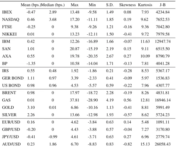
Table 1 reports descriptive statistics for daily returns. All the assets have mean and median returns close to zero. Returns on interest rates are obtained as log changes in the price of implicit zero coupon bonds having the value of an interest rate as a yield. In terms of standard deviation, the sample range is higher for AUD/USD (18.7), IRS (18.0) and US BOND (17.1) and lower for JPY/USD (13.2), EUR/USD (13.4), SILVER (13.8) and the interest rate on the GERMAN BOND (13.9). The unconditional standard deviation is relatively similar for assets in the same class, except for commodities, where GAS (4.19) and OIL BRENT (2.28) are more volatile than GOLD (1.13) and SILVER (1.93). NASDAQ is more volatile than other stock market indexes and AXA is the most volatile stock. The $US exchange rate for the Australian dollar has higher standard deviation than the one for the euro, British pound or Yen. AUD/USD, SILVER, GOLD and NIKKEI have significant negative skewness, while GAS, AXA, JPY/USD and NASDAQ have high positive skewness. For all the assets considered the kurtosis is high, implying that the return distributions have much thicker tails than the Normal distribution. Kurtosis is specially large for AUD/USD, GAS, IBM and AXA while EUR/USD, while the interest rate of the GERMAN BOND and the JPY/USD exchange rate have lower kurtosis. Together with a large sample size, these values for skewness and kurtosis lead to a vary large Jarque-Bera statistic, rejecting the assumption of Normality in all cases.
5
Parameter estimates
To perform a VaR analysis we estimate four volatility models: GARCH, GJR-GARCH, APARCH and FGARCH under each of the different probability distributions assumed for the innovations: Normal, Student-t, skewed Student-t, skewed Generalized Error, JohnsonSU, skewed
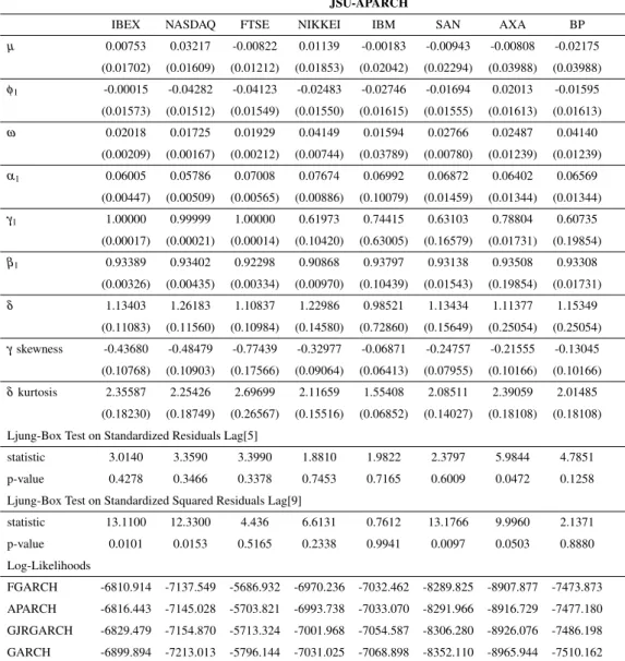
Generalized-t and Generalized Hyperbolic skew SGeneralized-tudenGeneralized-t-Generalized-t disGeneralized-tribuGeneralized-tions. In Table 2 we reporGeneralized-t esGeneralized-timaGeneralized-tion resulGeneralized-ts of the APARCH model under the JohnsonSU probability distribution for the stock market indexes
and for individual stocks.7 An AR(1) model was specified for the conditional mean return in all
7The estimation results for this volatility model under the different probability distributions for the stock market indexes and for individual stocks in our sample are reported in Tables A2 and A3 of the Online Appendix.
cases.8
The model is particularly successful in capturing the autocorrelation and heteroscedasticity exhibited by the data. The Ljung-Box Q statistic for nine lags computed on the standardized residuals does not show evidence of autocorrelation at 1% significance level. The same statis-tic computed with nine lags on the squared standardized residuals is not significant at 1% except for IBEX and SAN, both of them for a narrow margin. The autoregressive effect in volatility is strong, with aβ1-parameter generally above 0.90, suggesting strong memory effects. The
coeffi-cientγ1 is positive and statistically significant for all series, indicating the existence of a leverage
effect for negative returns in the conditional variance. Estimates ofγ1 are close to 1 for IBEX,
NASDAQ and FTSE, suggesting that only negative shocks contribute to volatility. The skewness parameter (γ) of the JohnsonSU distribution is less than 1 for the four stock indices, suggesting
the convenience of incorporating negative asymmetric features in the probability distribution in order to model innovations appropriately. Finally, theδ-parameter takes values between 0.97 and
1.54, being significantly different from 2 in most cases. This result is in line with those of Tay-lor (1986), Schwert (1990) and Ding et al. (1993) who indicate that there is substantially more correlation among absolute returns than among squared returns, a reflection of the ’long memory’ of high-frequency financial returns. Our estimates of the APARCH model for the different asset classes (not shown in the tables) suggest that, contrary to standard practice, we should model the conditional standard deviation for stock market indexes, individual stocks and metals, the condi-tional variance (δ =2) for interest rates, and a value between conditional standard deviation and
variance (δ=1.5) for energy commodities and exchange rates. We obtained the same parameter
estimates using MatLab, R, Eviews and Gretl.
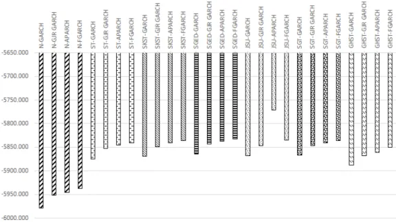
In the lower panel we present the log-likelihood values of the four volatility models (GARCH, GJR-GARCH, APARCH and FGARCH) under the JSU probability distribution. For individual stocks as well as for stock indexes the least restricted FGARCH model achieves the highest like-lihood, followed by APARCH, GJR-GARCH and GARCH models. A similar result was obtained for all other assets and all the probability distributions, and Figure 1 shows mean log-likelihood values for each model specification across the set of assets. Likelihood differences are statistically significant for many assets, with the GARCH specification being rejected against GJR-GARCH, and the latter being rejected against the APARCH and FGARCH specifications. The exceptions are exchange rates and long-term interest rates, for which it is hard to discriminate among volatil-ity specifications. On the other hand, likelihood differences between APARCH and FGARCH models are generally not statistically significant.
6
VaR Performance
We now analyze the VaR performance of our estimated models restricting our attention to the left tail of the distribution and the 1% significance level. The choice of the α =1% level is a
compromise between trying to capture extreme events and trying to avoid a too low number of exceptions. Results for alternative significance levels are available from the authors upon request.
8Most computations were performed with the rugarch package (version 1.3-4) of R software (version 3.1.1), de-signed for the estimation and forecast of various univariate ARCH-type models. The exception is the estimation of models under the skewed Generalized-t and Generalized Hyperbolic skew Student-t distributions for which we used the sgt package (version 2.0) and the SkewHyperbolic package (version 0.3-2), respectively.
Considering the left tail is not a trivial choice, since results for both tails may differ significantly for asymmetric return distributions.
We estimate the one-step ahead VaR parametrically as: VaRα,t =µt(θ) +σt(θ)F−1(α|θ),
where µt(θ) represents the conditional mean, σt(θ) is the conditional standard deviation and
F−1(α|θ)denotes the corresponding quantile of the distribution of the standardized innovations zt at a givenα% significance. Every day we compute 1-day ahead 1% VaR forecasts over the last
five years in the sample: 2011-2015 (1260 data observations). Models were reestimated every 50 days, a choice based on several arguments: 1) estimating each day is computationally demanding because we jointly estimate the parameters for the mean return, its conditional variance, and for the probability distribution of the return innovation,9 2) we work with an ”expanding window” that starts with a 11-year sample (2000-2010) and an out-of-sample of 5 years (2011-2015), and adding a single data to the 10-year sample does not change the estimated parameters, 3) our choice is in line with that made by different authors, like Giot and Laurent (2003a), and Diamandis et al. (2011) among others, who reestimate their models every 50 days. However, we report below some VaR backtesting results obtained reestimating the models daily.
After that, we examine the performance of VaR models through standard tests: the uncondi-tional coverage test of Kupiec (1995), the independence and condiuncondi-tional coverage tests of Christof-fersen (1998), the Dynamic Quantile test of Engle and Manganelli (2004), as well as by evaluating the Asymmetric Linear Tick loss function (AlTick) proposed by Giacomini and Komunjer (2005). For a comprehensive review on VaR forecasting and backtesting, see Nieto and Ruiz (2015).
The unconditional coverage test introduced by Kupiec (1995) is based on the number of vio-lations, i.e. the number of times (T1) that returns exceed the predicted VaR over a period of time
T for a given significance level. If the VaR model is correctly specified, the failure rate ( ˆπ =TT1)
should be equal to the pre-specified VaR level (α). The null hypothesisH0 :π=α is evaluated through a likelihood ratio test:
LRuc=−2 ln L(Πα) L(Π)b ! =−2 ln (1−α)T0αT1 (1−πˆ)T0πˆT1 T→∞ −→ χ12 whereT0=T−T1.
Two other tests by Christoffersen (1998) examine whether VaR exceedances are indepen-dent. We consider two states of nature each period: state 0 if the return does not fall below VaR: rt >VaR(α), and state 1, if rt <VaR(α). For the alternative hypothesis of VaR
ineffi-ciency, it is assumed that the process of violations It(α), where It(α) =1 if rt <VaR(α) and
It(α) =0 otherwise, can be modeled as a Markov chain with πi j =Pr[It(α) = j|It−1(α) =i].
Let us then denote byTi j the number of observations in state j after having been in state i in
the previous period, and define T0=T00+T10 and T1 =T11+T01. The two probabilities of a
VaR excess (state 1), conditional on the state of the previous periodπ01andπ11are estimated by
ˆ
π01=T01/(T00+T01)and ˆπ11=T11/(T10+T11). Under the null hypothesis of independence of
VaR exceedances:π01=π11=π= (T11+T01)/T, the likelihood function isL(Π) = (b 1−πˆ)T0πˆT1.
The likelihood under the alternative hypothesis is: L(Πb1) = (1−πˆ01)T00πˆ
T01
01 (1−πˆ11)
T10πˆT11
11 . The
independence test of Christoffersen (1998) is a test of the hypothesis of serial independence in VaR exceedances against a first-order Markov dependence. The likelihood ratioLRind statistic is:
9The computation is especially laborious for the FGARCH volatility specification and the GHST probability distri-bution.
LRind=−2 ln(L(Π)b /L(Πb1))with a distributionχ12. The conditional coverage test is based on the
likelihood ratio statistic, LRcc=−2 ln(L(Πα)/L(Πb1)) =LRuc+LRind, which is asymptotically
distributedχ22.
While the conditional coverage test is easy to use, it is rather limited for two main reasons,i) the independence is tested against a very particular form of alternative dependence structure that does not take into account a dependence of order higher than one,ii) the use of a Markov chain only considers the influence of past violationsIt(α) and not the influence of any other
exoge-nous variable. The Dynamic Quantile Test proposed by Engle and Manganelli (2004) overcomes these two drawbacks of the conditional coverage test. These authors suggest using a linear re-gression model that links current violations to past violations. Let us define the auxiliary variable:
Hitt(α) =It(α)−α, so that Hitt(α) =1−α ifrt <VaRt|t−1(α)andHitt(α) =−α otherwise.
The null hypothesis of this test is that the sequence of hits (Hitt) is uncorrelated with any
vari-able that belongs to the information setΩt−1available when the VaR was calculated and it has a
mean value of zero, which implies, in particular, that the hits are not autocorrelated. The Dynamic Quantile test is a Wald test of the null hypothesis that all slopes in the regression model,
Hitt(α) =δ0+ p
∑
i=1 δiHitt−i+ q∑
j=1 δp+jXj+εtare zero, whereXjare explanatory variables contained inΩt−1. The test statistic has an
asymp-totic χp2+q+1 distribution. In our implementation of the test, we use p=5 and q=1 (where X1=VaR(α)) as proposed by Engle and Manganelli (2004). By doing so, we are testing whether
the probability of an exception depends on the level of the VaR.
To evaluate the consequences of a VaR exceedance, we use the Asymmetric Linear Tick loss function (AlTick) proposed by Giacomini and Komunjer (2005), which takes into account the magnitude of the implicit cost associated with VaR forecasting errors. Hence, it takes into con-sideration not only the returns that exceed the VaR, but also the opportunity cost produced by an overestimation of VaR. When there are not exceptions, the loss function penalizes for the excess capital retained:
Lα(et+1) =
(
(α−1)et+1 ifet+1<0
αet+1 ifet+1≥0
whereet+1=rt+1−VaRt+1. Giacomini and Komunjer use the asymmetric linear loss function
withα equal to the significance level used to forecast VaR. The AlTick function can be seen as
the implicit loss function whenever the object of interest is a forecast of a particular quantile of the conditional distribution of returns. That way, a VaR model is preferable if it has a lower average value of the loss function.
The different combinations of probability distributions and volatility specifications, applied to each of the 19 assets considered, yield a large number of VaR tests and it is hard to summarize so much information in order to achieve some clear-cut conclusion on the adequacy of each model. We will proceed in the next section along four lines: i) the frequency of rejections of a given model when applying each test to the set of assets, ii) how often thep-value of a given test decreases when switching between two models differing in either the probability distribution or the volatility specification, iii) selecting the preferred models by a concept of precedence among VaR models we introduce below, iv) implementing a Model Confidence Set approach to select the preferred
VaR models for each asset. This approach is based on the use of a specific loss function. The first three criteria are based on properties of the tests for validation of VaR forecasts, while the fourth criterion deals with the size of the sample returns exceeding the estimated VaR.
6.1 Frequency of violations
Violation rates for VaR close toα =0.01 (13 violations) are desirable. Further, under the Basel
Accord, models that over-estimate risk are preferable to those that under-estimate risk levels. In our case, less than 20 violations of VaR would define the ’green zone’, between 20 and 50 vio-lations would correspond to the ’yellow zone’ and the ’red zone’ would be defined by more than 50 violations.10 In fact, falling inside the green zone is not necessarily a good thing if the number of violations of VaR is too low, since then the financial institution would be taking an excessive opportunity cost of capital.
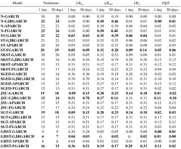
Table 3 contains a summary of backtesting results, showing for each model specification the median number of VaR violations and the number of rejections of each test across the set of 19 assets.11 The expected number of violations (13) falls in the green zone, so a good model should be in that zone. Across the 76 VaR analysis performed (4 volatility specifications and 19 assets) models under the Normal distribution fell in the green zone 26 times out of 76 (34%), 55 times under the Student-t distribution (72%), 72 times under SKST (95%), 69 times under SGED (91%), 75 times under JSU (99%), 73 times under SGT (96%) and 70 times under GHST (92%). All the other models fell in the yellow zone. The Normal distribution falls too often in the yellow zone. The frequency of the Student-t distribution to produce a model in the green zone was not very high either. All other probability distributions lead frequently to models in the green zone. We never observed a model to fall in the red zone for any asset.
Figure 2 shows the median number of VaR violations for each combination of probability distribution and volatility specification. The Normal distribution leads to the largest median num-ber of violations (22) across the 76 models (4 volatility specifications and 19 assets). Since the expected number of violations is 13, the Normal distribution clearly underestimates the level of risk. The GHST distribution produces the lowest median number of violations (10), with a clear overestimation of risk. All the other probability distributions have a median number of violations around 15, with a slight underestimation of risk that is more evident for the Student-t distribution. We can say that except by the Normal and GHST distributions, all other distributions perform well. Being more specific, the median frequency of violations is 1.75% for models with Normal innovations, 1.27% for Student-t innovations, 1.19% for skewed Student-t, skewed Generalized Error and skewed Generalized-t innovations, 1.11% for Johnson SU innovations and 0.79% for
Generalized Hyperbolic skew Student-t innovations. According to the frequency of violations, the
10In terms of Basel Accord, based on a sample of 250 observations, if the number of exceptions is less than, or equal to 4 (the green zone), the test results are consistent with an accurate model and the possibility of erroneously accepting an inaccurate model is low. At the other extreme, if there are 10 or more exceptions (the red zone), the test results are extremely unlikely to have resulted from an accurate model, and the probability of erroneously rejecting an accurate model on this basis is remote. In between these two cases we have the yellow zone, where the backtesting results could be consistent with either accurate or inaccurate models, and the supervisor should encourage a bank to present additional information about its model before taking action. We have applied to these thresholds a scale factor based on our sample size of 1260 observations.
11Tables A4-A7 in the Online Appendix show for each asset the number of observed violations of VaR forecasts, the statistic andp-value of each test for each combination of volatility model and probability distribution for the innovations.
unbounded JohnsonSU distribution shows the best behavior among the asymmetric probability
distributions. The performance of GHST might be acceptable under some criteria, although it would lead to an excessive opportunity cost of capital.
Differences among volatility specifications are much smaller. Models with a GARCH specifi-cation fell 114 times out of 133 cases (7 probability distributions and 19 assets) in the green zone (86%), 109 times for the GJR–GARCH (82%), 108 times for APARCH (81%) and 109 times for FGARCH (82%) out of 133 VaR analysis. The median number of violations was 15, 15, 16 and 16, respectively, very similar across volatility specifications. The frequency of violations for all volatility specifications is 1.19% for GARCH and GJR-GARCH, and 1.27% for APARCH and FGARCH models. This result already suggests the need to be careful when choosing an appropri-ate probability distribution for return innovations. Selecting the best volatility specification is also important, but the consequences of not making the right choice do not seem to be so crucial.
It is also interesting to examine the performance by asset type. Most models tend to overesti-mate risk in energy commodities (OIL and GAS). The median number of violations over the set of 28 models (7 probability distributions and 4 volatility specifications) is 7 for OIL and 5 for GAS (see Figure 3). A similar result is obtained for the GBP/USD and AUD/USD exchange rates, with a median number of 10 violations in both cases, which is not the case for the two other exchange rates.12 But the general result is that more often than not, models tend to underestimate risk in all assets, with a number of violations above the expected value of 13. Underestimation is spe-cially evident in the non-industrial metals (GOLD and SILVER) and some Spanish stock market variables (SAN and IBEX).
Using data for NASDAQ 100, Table 4 shows that differences in backtesting statistics forVaR1%
when models are re-estimated every day or every 50 days are small. The largest differences arise for FGARCH volatility specifications and for the DQT test. The similarity in results reinforces our choice to re-estimate models every 50 days.
A quick glance at Table 3 already reveals that the number of rejections of the four tests is highest under the assumption of a Normal distribution for return innovations. However, comparing all the other models in terms of backtesting results is far from obvious. The next sections try to select the best performing model specifications using different approaches.
6.2 Switching between VaR models
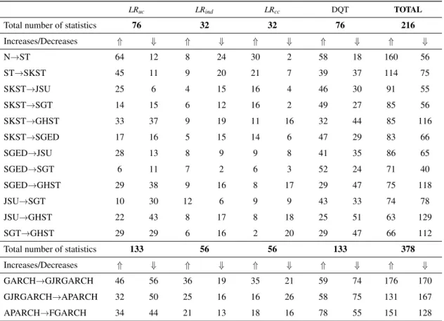
In a comparative analysis of VaR forecasting performance, applyingn=4 tests tom=28 alterna-tive models representing the dynamics ofk=19 assets, we will generally havem·n·k=2128 test outcomes. For 19 assets, we have a total of 216 tests performed under each probability distribution, and 378 tests under each volatility specification.13 They produce a large amount of information, and we need to design ways to summarize that information in order to be able do draw some conclusion on the relative merits of each probability distribution and each volatility specification. This is what we do in the next sections.
We start by comparing, for each of the four VaR tests described above (Kupiec, independence, conditional coverage and Dynamic Quantile tests), thep-values of the test statistics for models that differ in either the probability distribution for the innovations or in the specification of volatility
12The median number of violations is also below 13 for BP, but it is so close to that target that we have to consider the difference as sampling error.
dynamics. In these tests the null hypothesis is H0: the VaR model is ’appropriate’, in some sense that is specific to each test. As the probability of finding a similar sample with a more contrary evidence to H0, thep-value gives us a numerical indication on how favorable is our sample to H0. Hence, when comparing any two VaR forecasting models, we should prefer the one with a higher
p-value in VaR validation tests. To summarize the results of this analysis, Table 5 displays the number of cases in which thep-value of the test statistic increases or decreases when we change either the probability distribution or by the specification of the volatility model. We cannot make any formal testing, but by comparingp-values, we are searching for patterns that might suggest that a particular model is preferred over a given alternative.
If we consider all the possible specifications sharing the same probability distribution for re-turn innovations, we see that switching from a Normal to a Student-t distribution for rere-turn inno-vations increases thep-value of VaR tests in 160 out of a total of 216 comparisons, suggesting in those cases a more accurate VaR model.14 Even though the test statistics are obviously subject to sampling error, that frequency of increases inp-value suggests that, as expected, the Student-t dis-tribution is generally more appropriate than the Normal disdis-tribution to represent financial returns. Switching from the symmetric to the skewed Student-t distribution achieves a further increase in
p-value in 114 comparisons, while decreasing in 75 cases. Moving from the asymmetric Student-t to the unbounded Johnson distribution achieves an increase in 91 cases while decreasing in 55 cases. Switching from the asymmetric Student-t (SKST) to other asymmetric distributions (SGT, JSU, SGED), thep-value increases more often than otherwise. On the contrary, if we switch from the SKST, SGED, JSU or SGT distributions to the GHST distribution, the opposite happens, with thep-value usually decreasing. Hence, we consider the SKST, SGED, JSU and SGT distributions to be preferable to GHST. Between these asymmetric distributions, switching to JSU or SGT leads to an increase inp-value in a greater number of cases.
Among volatility models, switching from the symmetric GARCH to GJR-GARCH increases thep-value of the statistic in 176 out of 378 comparisons. The p-value increases in 131 cases when switching from GJR-GARCH to APARCH, but it decreases in 167 cases. On the other hand, if we move from the APARCH to the FGARCH model, thep-value increases in 151 out of 378 cases, decreasing in 128 cases. Overall, the FGARCH model seems to be the preferable volatility specification. Percent differences between the number of cases in which the value of the test statistic increases or decreases when switching between volatility models are much smaller than the ones obtained when switching between two probability distributions. This suggests again that, according to the performance of the models for VaR estimation, the specification of the volatility dynamics is not as important as the choice of probability distribution for the innovation in returns.
6.3 A ranking based on backtesting results
In the previous section we have applied four tests for VaR performance: the unconditional likelihood-ratio test, the independence test, the conditional coverage test, and the dynamic quantile test, and each test has been run for a variety of models and assets. In this section we evaluate the adequacy of the different models considered for VaR forecasting by comparing the specific situations in
14The number of possible comparisons arises from applying all the VaR tests to all the assets. The difference between this number and the sum of increases and decreases in thep-value is the number of cases in which thep-value of the test statistic does not change.
which each model has been rejected by each test.15
Definition 1 Given a confidence level between 0 and 1, we say that model M2δ-precedes model M1 in VaR performance if i) M1 has been rejected in at least as many cases as M2, and ii) in a percentage of at leastδ of the cases when M2 is rejected by a test, M1 is also rejected.
Notice that δ does not need to be related to the confidence level at which VaR validation
tests are implemented. We would expectδ to be around .90 in most practical applications. The
interesting feature of this precedence criterion is that it compares any two model specifications across all the statistical tests and assets, thereby allowing us to achieve some robust results. The criterion could accommodate different weights for each test depending on the relevance we want to assign them. The precedence criterion would then use the number of rejections in each test, weighted by relevance. An interesting possibility would consist of assigning a larger weight to tests having a larger ability to discriminate among models. Weights could also be chosen as a bounded function of the size of the test rejection, either in terms of the test statistic or thep-value of the test.
The precedence criterion could also be used to choose among forecasting models that are required to satisfy some condition to be considered acceptable. For instance, if competing models are used over a number of periods to forecast a given variable, and there is a maximum forecast error that is acceptable, the precedence relationship would be based on the number of periods in which each model exceeds that error threshold.
Table 6 contains the information needed to establish precedence comparisons across VaR mod-els. The upper panel corresponds to implementing the VaR validation tests at 99% confidence, while the lower panel has been obtained with test results at 95% confidence. In each panel, the up-per part compares the rejections of models using probability distributions D1 (left) and D2 (right) when combined with all the volatility specifications. The lower part compares the rejections of models made up with volatility specifications M1 (left) and M2 (right) when combined with all the probability distributions. The first two columns of each panel in Table 6 show the number of cases when the two probability distributions or the two volatility specifications listed in the first column have been rejected by the data when applying the unconditional coverage tests of Kupiec. The third column displays the percentage of rejections of D2 (M2) that were also rejections of D1 (M1). We will conclude that the the probability distribution (or the volatility specification) with the lower number of rejections precedes the competitor when this percentage is below a pre-specified threshold forδ. The following three columns refer to the independence tests, and the next columns
come from the conditional coverage test and the Dynamic Quantile test. The final three columns aggregate the number of rejections across tests. For instance, if we take a thresholdδ =.90, the
independence test of Kupiec rejected 36 models made up with the Normal distribution and just 7 models with the Student-t distribution. Besides, those 7 models rejected under the Student-t distri-bution were also rejected under a Normal distridistri-bution. Hence, the Student-t distridistri-bution precedes the Normal distribution according to this test. The independence test rejected 7 models made up with either the Normal or the Student-t distributions. In 5 of the 7 rejections under a Student-t distribution for return innovations the model was also rejected under a Normal distribution. That
15However, some tests might not be feasible in some samples, which explains the empty cells for the independence test and the conditional coverage test in Tables A4 to A7 of Online Appendix.
ratio is 5/7=0.714 so that, according to the independence test, we could not conclude that models with a Student-t distribution for return innovations precede models with a Normal distribution.
The number of pairwise comparisons between probability distributions or between volatility specifications is very high because they could be made in both directions, so we show in Table 6 the more interesting ones. For instance, we do not explicitly show the comparisons between the Normal distribution and asymmetric distributions because the latter always precedes the former. Similarly, we do not show pairwise comparisons between Student-t and any asymmetric distribu-tion other than the skewed Student-t (SKST) because the skewed Student-t tends to precede the standard Student-t, and the majority of asymmetric distributions precede in turn over the skewed Student-t distribution.16
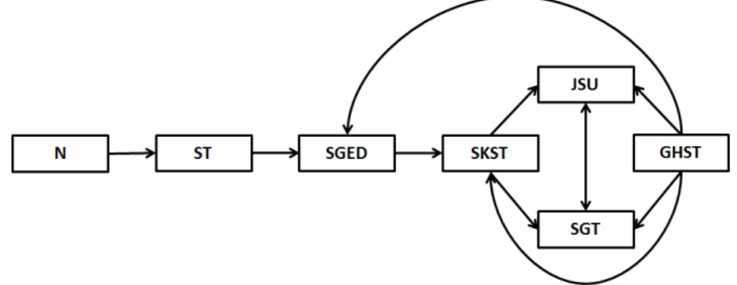
Taking into account the aggregate results across the four tests we can summarize the compar-isons atα =95% as in the diagram:
Diagram 1: Precedence relationship among probability distributions from aggregate results across the four test atα=95%. Each arrow head points to a model that precedes the model where the
arrow originates. A two-headed arrow indicates two models that do not precede each other.
No matter whether we takeα =99% orα =95%, the Normal, Student-t, SKST and SGED
distributions are preceded by other alternatives, specially JSU and SGT. We observe that JSU and SGT distributions seem to precede over all others, while not being preceded by each other. According to thisδ-precedence criterion the GHST distribution is judged again not to be
appro-priate for VaR estimation, since it is preceded by the rest of asymmetric distributions. The Normal distribution is also preceded by all other distributions.
At α =99% there is not a clear precedence ordering between volatility specifications. For α=95% the FGARCH specification seems to precede all others but, once again, differences are
not as clear as when comparing probability distributions.
A preference for APARCH and FGARCH models against standard GARCH and GJR-GARCH has been a constant throughout our analysis up to this point. So, a robust conclusion is the need to incorporate a leverage effect in volatility and, possibly more important, the convenience to model standard deviations, rather than variances. The preference for asymmetric probability distributions in Table 6 is also consistent with results in Table 5 when comparingp-values of the test statistics.
16Even though
δ-precedence is not a transitive relationship, it seems safe to focus on the models that tend to be
Both analysis are based on the same information, but they use it in a very different fashion. Nothing guarantees that the conclusions on the preferred probability distributions should be the same in both analysis. On the contrary, this coincidence should be seen as a proof of the robustness of such preference.
6.4 Model Confidence Sets
The availability of several model specifications being able to adequately describe the unobserved data generating process (DGP) opens the question of selecting the ’best fitting model’ according to a given optimality criterion. Recently, significant effort has been placed on developing testing procedures being able to deliver the ’best fitting’ models among a set of alternatives. One of the first proposals was Diebold and Mariano (1995), but it is not applicable when the forecasts come from nested models or when the forecasts are calculated from semiparametric or non parametric methods (Giacomini and Komunjer, 2005). This has been overcome by the Reality Check (RC) approach of White (2000), the Stepwise Multiple Testing procedure of Romano and Wolf (2005), the Superior Predictive Ability (SPA) test of Hansen and Lunde (2005), the Conditional test of Gi-acomini and White (2006), and the Model Confidence Set (MCS) procedure developed by Hansen et al. (2011). All these approaches are relevant from an empirical point of view, especially when the set of competing alternatives is large.
We implement the Model Confidence Set (MCS) procedure developed by Hansen et al. (2011). It is a general approach to model selection that it does not require that the “true” model must be available as one of the competing models. The MCS procedure consists of a sequence of tests to construct the ’Set of Superior Models’ (SSM). At each step the worst model is eliminated, until the hypothesis of Equal Predictive Ability (EPA) is not rejected for any of the models in the current SSM. At each step, each element in the SSM is characterized as having better predictive ability than models not in the set. The SSM has an interpretation similar to a confidence interval for a parameter in the sense that, with a given level of confidence, the SSM contains the best model. The EPA test statistic is evaluated under a given loss function, so that it is possible to test models on various aspects depending on the chosen loss function.17
Formally, the loss function`i,t associated to the i-th model`i,t =`(Yt,Yˆi,t)measures the cost
associated to the difference between the observation at timet,Yt, and ˆYi,t the output of model i
at timet. The MCS procedure starts from an initial set of models ˆM0 of dimensionmmade up by all combinations of probability distributions and volatility specification considered in previous sections. Then, for a given confidence level 1−α, we obtain a smaller set, the superior set of
models, SSM, ˆM1−∗ α of dimensionm∗≤m. Let us denote bydi j the loss differential between
modelsiand j,di j,t =`i,t−`j,t,i,j=1, ...,m,t=1, ...,T. The EPA hypothesis for a given set of
modelsMcan be formulated: H0,M: ci j=0, for all i,j=1, ...,m, against the alternative: H1,M:
ci j6=0, for somei,j=1, ...,m, whereci j=E(di j)is assumed to be finite and not time dependent.
This hypothesis can be tested using the test statistic [Hansen et al. (2011)],ti j =d¯i j/
q
c var(d¯i j)
17We believe that the opportunity cost of overestimating VaR is non trivial. The AlTick loss function not only penalizes underestimation but also risk overestimation, because of the excess capital retained, and therefore we prefer it over other loss functions, such as those proposed by Lopez (1998, 1999) and Sarma et al. (2003) which only penalize risk underestimation. However, it would be worthwhile to explore other loss functions that might focus on different characteristics of VaR forecasts.
fori,j∈M, where ¯di j=n−1∑tn=1di j,t measures the relative sample loss between thei-th andj-th
models, whilevarc(d¯i j)is a bootstrapped estimate ofvar(d¯i j).
Following Hansen et al. (2011) and Radovanov and Marcikic (2014) we calculate the boot-strapped variances by a block-bootstrap procedure. To that end, we divide the time series of 1260 data observations into overlapping blocks of lengthp, which is usually estimated as the maximum number of significant parameters in an AR(p) process fitted to all thedi j terms. Since financial
returns exhibit little linear autocorrelation, an AR(1) is enough to capture the dependence struc-ture, and we usedp=1 to resample individual observations. We checked that using a block length of 2 does not change significantly the characterization of the MCS. As discussed in Hansen et al. (2011) the EPA null hypothesis maps naturally into the statistic,TR,M =maxi,j∈M|ti j|. Since the
asymptotic distributions of this test statistic is nonstandard, the relevant distribution under the null hypothesis was estimated using a bootstrap procedure similar to that used to estimatevar(d¯i j).
Table 7 reports the frequency by which each probability distribution and each volatility spec-ification enter into the Superior Set of Models for each asset.18 Tests are performed at the 90% confidence level, using a block-bootstrap procedure of 10000 resamples with a block length of 1. The table shows that for some assets, like NASDAQ 100, FTSE 100, EUR/SD and JPY/USD, the SSM includes a variety of distributions and volatility specifications. That indicates that the one-step ahead 1% VaR forecasting performance of the competing combinations of probability distribution and volatility specification is relatively similar, suggesting that for these assets the use of simple models for VaR forecasting may be justified. The SGT, JSU, SGED and GHST distribu-tions are the ones that enter most often into the MCS of the set of assets considered. Among the volatility models, FGARCH and APARCH seem to describe quite well the behavior of financial time series, although the symmetric GARCH also enters into the MCS quite often. Concerning the distribution specifications, we observe that the MCS confirms the common finding that the Normal distribution provides a poor description of the behavior of financial time series. Under the AlTick loss, the skewed Generalized-t and skewed Generalized Error distributions perform better than the Generalized Hyperbolic skew Student-t. Definitely, the Normal, Student-t and skewed Student-t distributions do not seem to be appropriate for VaR forecasting for the wide set of financial assets considered in this paper.
6.5 10-day VaR forecasting
In spite of the Basel Committee on Banking Regulation (2009) switch to require 10-day VaR estimation, there is not much work yet exploring the performance of alternative VaR models. De-giannakis and Potamia (2017) and DeDe-giannakis et al. (2013) analyze a number of issues regarding 10-day VaR and expected shortfall forecasting. Degiannakis and Potamia (2017) conclude that the use of intra-day data does not lead to better risk estimates. They also obtain a preference for skewed distributions and a GARCH volatility specification, as well as a better forecasting perfor-mance at 97.5% than at 99% significance level. Degiannakis et al. do not find an improvement in the accuracy of risk estimation from using long memory volatility models.
A major difficulty with multi-step VaR forecasting is that the use of non-overlapping samples drastically reduces the number of VaR observations. To solve this limitation, Barone-Adesi et al.
18Table A8 in the Online Appendix shows the values of the AlTick loss function using for the different model specifications and assets.
(1998, 1999, 2002) propose the FHS method that extends the idea of volatility adjustment to multi-step historical simulation, using overlapping data in a way that does not create blunt tails for the
h-day portfolio return distribution,h>1. The method consists in applying a statistical bootstrap to the standardized residuals of a parametric dynamic model of returns, to simulate log returns each day over the desired risk horizon. Typically, the model used for FHS incorporates a specification of the GARCH family for volatility dynamics. The filtering involved in FHS allows forh-day return distributions to be generated from overlapping samples, since the bootstrap allows for increasing the number of observations used for building theh-day return distribution. The advantages of the FHS approach are 1) it captures current market conditions by means of the volatility dynamics, 2) no assumptions need to be made on the distribution of the return innovations, and 3) the method allows for the computation of any risk measure at any investment horizon of interest because one can generate as manyh-day returns as one likes. The drawback is that we can only apply to these multi-period returns the unconditional coverage test.
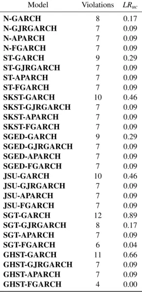
Table 8 shows the performance of the models in 10-day ahead 1% VaR forecasts for NASDAQ 100. We use an expanding window to estimate the model, starting with the 2915 observations from the 10/2/2000-12/2/2011 period. Each day we add a new observation, we estimate the models and apply filtered historical simulation (FHS) to simulate 5000 10-day future returns from which we compute VaR forecasts. The forecasting exercise extends over 1260 days, the last five years in our sample, 12/5/2011-9/30/2016, obtaining daily 10-day VaR forecasts.19 The results we obtain for 10-day VaR forecasts can be summarized as follows: i) VaR violation rates are below their theo-retical value of 13, indicating an overestimation of risk for all models;ii) models with symmetric and models with asymmetric distributions perform similarly at VaR forecasting, although GARCH volatility specifications have a better performance, with violation rates being systematically closer to their expected value;20 iii) even though model specifications are not rejected, unconditional coverage test p-values are low, except for GARCH volatility.
Some of the daily changes in VaR at short horizons may be due to pure noise that gets wiped out in longer horizons. That explains that 10-day VaR forecasts are smoother than 1-day VaR fore-casts and differences in estimates across models are smaller. Furthermore, under a semiparametric method for VaR forecasting as FHS, the chosen model is less relevant than under a parametric methodology.
7
Conclusions
This paper extends previous work on the forecasting performance of alternative VaR models by considering four volatility specifications: GARCH, GJR-GARCH, APARCH and FGARCH and a set of asymmetric probability distributions: skewed Student-t, skewed Generalized Error, un-bounded Johnson, skewed Generalized-t and Generalized Hyperbolic skew Student-t distributions, some of them being relatively new to the financial literature. Standard symmetric distributions and GARCH models without leverage are also used as a benchmark. Our sample of daily data for as-sets of different nature for the January 2000-December 2015 period covers the recent financial crisis of 2007-2009.
19Thus, we have 10-day VaR observations that we can compare to the realized 10-day returns. 20This latter result is consistent with Degiannakis and Potamia (2017).