ROBUST MONOPOLY PRICING
By
Dirk Bergemann and Karl Schlag
July 2005
Revised April 2007
COWLES FOUNDATION DISCUSSION PAPER NO. 1527R
COWLES FOUNDATION FOR RESEARCH IN ECONOMICS
YALE UNIVERSITY
Box 208281
New Haven, Connecticut 06520-8281
http://cowles.econ.yale.edu/
Dirk Bergemanny Karl Schlagz First Version: May 2003
This Version: April 2007
Abstract
We consider a robust version of the classic problem of optimal monopoly pricing with incomplete information. In the robust version of the problem the seller only knows that demand will be in a neighborhood of a given model distribution.
We characterize the optimal pricing policy under two distinct, but related, decision
criteria with multiple priors: (i)maximin expected utility and (ii)minimax expected
regret. While the classic monopoly policy and the maximin criterion yield a single deter-ministic price, minimax regret always prescribes a random pricing policy, or equivalently, a multi-item menu policy. The resulting optimal pricing policy under either criterion is robust to the model uncertainty. Finally we derive distinct implications of how a monopolist responds to an increase in ambiguity under each criterion.
Keywords: Monopoly, Optimal Pricing, Robustness, Multiple Priors, Regret. Jel Classification: C79, D82
The …rst author gratefully acknowledges support by NSF Grants #SES-0095321, #CNS-0428422 and a DFG Mercator Research Professorship at the Center of Economic Studies at the University of Munich. We thank the Editor, Eddie Dekel and three anonymous referees for valuable comments. We thank Peter Klibano¤, Stephen Morris, David Pollard, Phil Reny, John Riley and Thomas Sargent for helpful suggestions. We are grateful to seminar participants at the California Institute of Technology, Columbia University, the University of California at Los Angeles, the University of Wisconsin and the Cowles Foundation Conference "Uncertainty in Economic Theory" at Yale University for many helpful comments. We thank the editor, Eddie Dekel, and three anonymous referees for their valuable comments.
yDepartment of Economics, Yale University, 28 Hillhouse Avenue, New Haven, CT 06511,
[email protected] and CEPR.
zDepartment of Economics, European University Institute, [email protected]
1
Introduction
In the past decade, the theory of mechanism design has found increasingly widespread applications in the real world, favored partly by the growth of the electronic marketplace and trading on the internet. Many trading platforms, such as auctions and exchanges implement key insights of the theoretical literature. Naturally, with an increase in the use of optimal design models, the robustness of these mechanisms with respect to the model speci…cation becomes an important issue. In this paper, we investigate a robust version of the classic monopoly problem of selling a product under incomplete information. The optimal pricing policy is the most elementary instance of a revenue maximizing problem.
We investigate the robustness of the optimal selling policy by enriching the standard model to account for model ambiguity. Instead of assuming a given demand distribution from which the buyer is drawn, the seller is only assumed to believe that the demand distribution will be in the neighborhood of a given model distribution. The enlargement of the set of possible distributions represents the model ambiguity.
The objective of this paper is to demonstrate that we can relax the rigid Bayesian model by considering robust decision making. We maintain a formal approach by building on axiomatic decision theory and obtain interesting new insights for monopoly pricing. The methodological insight is that robustness is generated by considering decision making under multiple priors. We then present rich comparative statics results in terms of the response of prices to an increase in ambiguity and uncover a novel role for menu pricing. Thus, the analysis of the robust pricing problem leads to testable hypotheses regarding the behavior of the seller.
Currently, there are two leading approaches to incorporate multiple priors into axiomatic decision making: maximin utility and minimax regret. The maximin utility approach with multiple priors is due to Gilboa & Schmeidler (1989). Here the decision maker evaluates each action by its minimum expected utility across all priors. The decision maker selects the action that maximizes the minimum expected utility. The minimax regret approach was …rst suggested by Savage (1951) and axiomatized by Milnor (1954). The minimax regret criterion was recently adapted to multiple priors by Hayashi (2006) and by Stoye (2006). Here the decision maker takes the maximum of the expected regret as the prior varies and chooses an action that minimizes the maximum expected regret.
In this paper, we shall analyze the optimal pricing policy under both criteria. We analyze the optimal policies when the ambiguity is represented by a neighborhood around a given model distribution. We de…ne the notion of a neighborhood through the usual metric of
weak convergence, the Prohorov metric. In the Prohorov metric two distributions are close to each other if they permit withlarge probabilitysmall changes in the valuations and with small probability large changes in the valuations. The analysis of the policies under the two decision criteria will reveal that either criterion leads to a robust policy in the following sense. We say that a candidate policy is robust if for any demand su¢ ciently close to the model distribution the di¤erence between the expected pro…t under the optimal policy for this demand and the expected pro…t under the candidate policy is arbitrarily small.
While the optimal policies under maximin utility andminimax regret share the robust-ness property, the response to ambiguity leads to distinct qualitative features. The pricing policy of the seller is obtained as the equilibrium strategy of a zero-sum game between the seller and adverserial nature. The strategy by nature selects the least favorable demand distribution to the objective of the seller. When the decision maker is maximizing the min-imum expect utility among the class of priors, the least favorable demand is always given by the distribution which puts maximal weight on the lowest quantiles subject to the re-striction that the selected distribution is in the neighborhood of the model distribution. As the objective of nature is to minimize the revenue of the seller, the least favorable demand is the one which minimizes the potential revenue at any possible price level. In particular as we increase the ambiguity represented by an increase in the size of the neighborhood, the least favorable demand increases the weight on the lower quantiles of the distribution. In consequence the best response of the seller always consists in lowering her price deter-ministically.
When we analyze the behavior under regret minimization, the optimal pricing policy is still determined by a zero-sum game between the seller and nature. The notion of regret modi…es the trade-o¤ for seller and nature. The regret of the seller is the di¤erence between the actual valuation of a buyer for the object and the actual revenue obtained by the seller. The regret of the seller can therefore be positive for two reasons: (i) a buyer has a low valuation relative to the price and hence does not purchase the object, or(ii)he has a high valuation relative to the price and hence the seller could have obtained a higher revenue. In the equilibrium of the zero-sum game, the optimal pricing policy for the seller has to resolve the con‡ict between the regret which arises with low prices against the regret associated with high prices. If the seller o¤ers a low price, nature can cause regret with a distribution which puts substantial probability on high valuation buyers. On the other hand, if the seller o¤ers a high price, nature can cause regret with a distribution which puts substantial probability at valuations just below the o¤ered price. It then becomes evident that a single
price will always expose the seller to substantial regret. Consequently, the seller can decrease her exposure by o¤ering many prices. This can either be achieved by a probabilistic price or, alternatively, by a menu of prices. With a probabilistic price, the seller diminishes the likelihood that the nature will be able to cause large regret. Equivalently, the seller can o¤er a menu of prices and quantities. The quantity element in the menu can either represent a true quantity in the case of a divisible object or a probability of obtaining the indivisible object.
The intuition regarding the price policy with regret is easy to establish in comparison to the revenue maximizing policy for a given distribution. An optimal policy for a given distribution of valuations is always to o¤er the entire object at a …xed price (a classic result by Harris & Raviv (1981) and Riley & Zeckhauser (1983)). In contrast, here the policy will o¤er many prices (with varying quantities). With a single price, the risk of missing a trade at a valuation just below the given price is substantial. On the other hand, if the seller were simply to lower the price, she would miss the chance of extracting revenue from higher valuation customers. She resolves this con‡ict by o¤ering smaller trades at lower prices to the low valuation customers. The size of the trade is simply the probability by which a trade is o¤ered or the quantity o¤ered at a given price. In the game against nature, the seller will have to be indi¤erent between o¤ering small and large trades. In terms of the virtual utility, the key notion in optimal mechanisms, this requires that the seller will receivezero virtual utility over a range of valuations. The resulting conditions on the distribution of valuations determine the least favorable demand. Importantly, an increase in ambiguity may now lead to an increase in the expected price. In the special case of linear model distribution we …nd that expected price increases if the optimal price under the model is low and decreases if the optimal price under the model is high.
From an axiomatic perspective, the maximin and minimax criteria represent di¤erent departures from the standard model of Anscome & Aumann (1963). The maximin de-cision criterion emerges by replacing the independence axiom with the weaker certainty independence axiom and adding a convexity axiom. Certainty independence requires that preferences between two given acts remain unchanged when mixing both with some con-stant act. The minimax regret criterion emerges by maintaining the independence axiom but relaxing the axiom of independence of irrelevant alternatives. It is postulated that the most preferred choice does not change when a new act is added as long as the additional act does not change the best outcome that can be achieved in each state. The weaker version holds vacuously in perfect information environment, i.e. when the state is known before
the choice. The convexity axiom and a variation of the betweenness axiom completes the characterization. Either approach allows to consider sets of distributions. Both maximin utility and minimax regret criteria do not contradict subjective expected utility theory, and we may interpret them as alternative axiomatic systems for selecting subjective priors.1
It should be pointed out that while the regret criterion seems to relate to foregone opportunities when the information is revealed ex post, this particular interpretation is solely an additional feature of the minimax regret model. Neither the axioms refer to foregone opportunities nor is it important whether or not ex post additional information becomes available. As in the case of maximin criterion of Gilboa & Schmeidler (1989), the minimax regret criterion in Hayashi (2006) and Stoye (2006) is completely characterized by a set of axioms.2
We conclude the introduction with a brief discussion of the directly related literature. The basic ideas of robust decision making (see De…nition 1) were …rst formalized in the context of statistical inference, in particular with respect to the classic Neyman-Pearson hypothesis testing. The statistical problem is to distinguish on the basis of a sample be-tween two known alternative distributions. The model misspeci…cation and consequent concern of robustness comes from the fact that each one of the two distributions might be misspeci…ed. Huber (1964), (1965) …rst formalized robust estimation as the solution to a minimax problem and an associated zero-sum game. In the economic context, a recent article by Prasad (2003) shows that the standard optimal pricing policy is not robust to small model misspeci…cations.
A recent paper by Bose, Ozdenoren & Pape (2006) determines the optimal auction in the presence of an ambiguity averse seller and ambiguity averse bidders. As we consider the optimal pricing problem the ambiguity aversion of the buyers is immaterial as there is no strategic interaction across buyers. Lopomo, Rigotti & Shannon (2006) consider a general mechanism design setting when the agents, but not the principal, have incom-plete preferences due to Knightian uncertainty. The notion of regret was investigated in mechanism design by Linhart & Radner (1989) in the context of bilateral trade as well
1
Klibano¤, M.Marinacci & Mukerji (2005) propose a related and smooth model of ambiguity aversion by enriching the multiple prior model with a belief over distributions and with an increasing transformation representing ambiguity aversion. The additional elements, belief and ambiguity index , render the analysis of multiple priors richer but also substantially more complex. In addition, the one dimensional representation of ambiguity in terms of the size of the neighborhood is not available anymore.
2In particular, the axiomatic approach to minimax regret is distinct from the ex-post measure of regret
due to Hannan (1957) in the context of repeated games or to the more behavioral approaches to regret o¤ered by Bell (1982) and Loomes & Sugden (1982).
as by Engelbrecht-Wiggans (1989) and Selten (1989) in the context of auctions. Linhart & Radner (1989) analyze minimax regret strategies in a bilateral bargaining framework. In contrast to the incomplete information environment here, the bulk of the analysis in Linhart & Radner (1989) is concerned with bilateral trade under complete information. In Engelbrecht-Wiggans (1989) and Selten (1989) the …rst and second price sealed bid auc-tions are analyzed incorporate regret for the bidders. Recently, Engelbrecht-Wiggans & Katok (2007) and Filiz & Ozbay (2006) present experimental evidence for regret in …rst price auctions.
The reminder of the paper is organized as follows. In Section 2 we present the model, the notion of robustness and the neighborhoods. In Section 3 we characterize the pricing policy under the maximin criterion. In Section 4 we characterize the pricing policy under the minimax criterion. We show that the resulting policies are robust under either criterion. Section 5 concludes with a discussion of some open issues. The appendix collects auxiliary results and the proofs.
2
Model
2.1 Monopoly
A seller o¤er an object for sale to an unknown demand. The demand is either generated by a single large buyer or by many small buyers. In the paper we focus on the case of a single large buyer and later show how the results generalize naturally to the case of many small buyers. Accordingly, the seller faces a single potential buyer with value v for a unit of the object. The valuevof the object is private information of the buyer and unknown to the seller. The valuation v of the buyer is an element of the unit interval, v2 [0;1].3 The marginal cost of production is constant and normalized to zero. The buyer wishes to buy at most one unit of the object.
The seller sets a pricep;thepro…t of selling the object at pricepif the valuation of the buyer is v is:
(p; v),pIfv pg; whereIfv pg is the indicator function specifying:
Ifv pg=
(
0; if v < p;
1; if v p:
3More generally, we assume that the value of the buyer is (known by the seller) contained in some closed
In the standard monopoly problem with incomplete information, the seller maximizes the expected pro…t for a given priorF over valuations. The expected pro…t given a distribution F is:
(p; F),
Z
(p; v)dF(v).
By extension, if the seller chooses a random pricing policy 2 R+, then the expected
pro…t is:
( ; F),
Z Z
(p; v)d (p)dF(v).
We denote the probabilistic price that maximizes the pro…t for given distribution F by
(F) so
(F)2 arg max
2 R+
( ; F).
A well-known result by Riley & Zeckhauser (1983) states that for every distributionF there exists a deterministic pricep that maximizes pro…ts, so:
(p (F); F) = max
2 R+
( ; F).
2.2 Ambiguity
In contrast to the standard model of monopoly pricing in which the seller acts as if the valuation of the buyer is drawn from a (subjective) distribution F, we assume that the seller faces ambiguity in the sense of Ellsberg (1961). The ambiguity is represented by a set of possible distributions, where the set is described by a model distribution F0 and
includes all distributions in a neighborhood of size " of the model distribution F0. The
magnitude of the ambiguity is thus quanti…ed by the size of the neighborhood around the model distribution.4
Given the model distribution F0 we denote by p0 = p (F0) a pro…t maximizing price
atF0. For the remainder of the paper we shall assume that(i) p0 is the unique maximizer
of the pro…t function for the model distribution, (ii) the pro…t function, (p; F0) at the
model distribution F0 is strictly concave near p0 and (iii) the density f0 is continuously
4This model of ambiguity permits at least two di¤erent interpretations. First, the"neighborhood around
the model distributionF0 can be understood as a model with multiple priors. Second, the"neighborhood can be viewed as an"perturbation of the original model distributionF0. By considering, the larger set of possible distributions the decision maker is protecting herself against measurment error and/or additional information which may slightly change the original model. We adopt throughout the …rst perspective, but it related to second perspective, prominent in statistical decision theory.
di¤erentiable nearp0. These regularity assumptions enable us the implicit function theorem
for the local analysis.
We consider two di¤erent decision criteria that allow for multiple priors: maximin utility and minimax regret. In either approach, the unknown state of the world is identi…ed with the valuev of the buyer.
Neighborhoods We describe " neighborhoods of the model distribution F0(v) by the
Prohorov neighborhood, denoted by P"(F0), and associated metric:
P"(F0) =fFjF(A) F0(A") +"; 8A [0;1]g, (1)
where the setA"denotes the closed"neighborhood of any Borel measurable setA. Formally, the set A" is given by
A"= v2[0;1] inf
y2Ad(x; y) " ;
whered(x; y) =jx yjis the distance on the real line. The Prohorov metric has evidently two components. The additive term"in (1) allows for asmall probability oflarge changes in the valuations relative to the model distribution whereas the larger setA" permitslarge probabilities of small changes in the valuations. The Prohorov metric is a metric for weak convergence of probability measures.5
Maximin Pro…t The seller maximizes the minimum pro…t by solving
m 2 arg max 2 R+
inf
F2P"(F0)
(p; F):
Accordingly, we say that m attains maximin pro…t. We refer to Fm as a least favorable demand given if
Fm2 arg min F2P"(F0)
( ; F)
so the least favorable demandFm minimizes pro…t under the policy :
Minimax Regret The regret of the monopolist at a given price p and valuation v of a buyer is de…ned as:
r(p; v),v pIfv pg=v (p; v); (2)
5
The Prohorov metric applies to discrete and continuous distributions. In contrast, the Kullback-Leibler distance only de…nes neighborhoods for continuous distributions. A related model is the contamination “neighborhood”N"(F0): N"(F0) =fFjF= (1 ")F0+"H for someH 2 R+g:Yet the contamination
The regret of the monopolist charging price pfacing a buyer with value v is the di¤erence between (i) the pro…t the monopolist could make if she were to know the value v of the buyer before setting her price and (ii) the pro…t she makes without this information. The regret is non-negative and can only vanish ifp=v. The regret of the monopolist is strictly positive in either of two cases: (i) the value v exceeds the price p, the indicator function is then Ifv pg = 1; or (ii) the value v is below the price p, the indicator function is then
Ifv pg= 0.
The expected regret with a random pricing policy when facing a distribution F is given by: r( ; F), Z r(p; v)d (p)dF(v) = Z vdF(v) Z (p; F)d (p). (3)
Thus, the probabilistic price is pro…t maximizing at F if and only if minimizes (ex-pected) regret when facing F: The pricing policy r 2 R+ attains minimax regret if it
minimizes the maximum regret over all distributions F in the neighborhood of a model distributionF0:6 r2 arg min 2 R+ sup F2P"(F0) r( ; F):
We refer toFr as aleast favorable demand given the pricing policy ifFrmaximizes regret under the pricing policy r:
Fr 2 arg max F2P"(F0)
r( r; F):
The notion of regret naturally extends to the case of many buyers as follows. The regret of the seller facing nbuyers is equal to the sum of the regret accrued over n buyers and n, possibly distinct, prices. While the seller is thus allowed to o¤er a di¤erent price to each buyer, the additivity of the regret implies that we can con…ne attention to price (distributions) which are identical across buyers.7
6
The fact that buyer value is contained in some known bounded set provides an upper bound on regret. If the support ofF 2 P"(F0)would not be uniformly bounded then regret would be unbounded onP"(F0) even if the support of F0 is contained in [0;1]. The neighborhood of the model F0 puts restrictions on the support. Imposing upper bounds on the willingness to pay are natural once one thinks about realistic applications.
7Alternatively we could restrict the seller to o¤er the same price to all buyers. The present analysis of
the single buyer then generalizes after imposing only that the marginal distribution of each buyer belongs toP"(F0):The least favorable demand will then involve all buyers realizing the same valuation.
2.3 Robust Pricing Policy
For a given model distributionF0 we identify a price policy as a class of probabilistic prices
f "gdependent on the size of the neighborhood ".
De…nition 1 (Robust Pricing Policy)
A pricing policy f "g is called robust if for each >0 there is " >0 such that: F 2 P"(F0) ) ( (F); F) ( "; F)< :
The above notion presents a formal criterion of robust decision making in the spirit of the statistical decision literature pioneered by Huber (1964). The robust policy is allowed to depend on the size"of the neighborhood.8 In contrast to minimax regret where pro…ts are compared to best choices ex-post, robustness involves comparing expected pro…ts to those attainable ex-ante when the valuation is drawn from a known distribution.
In the context of optimal monopoly pricing Prasad (2003) shows that the optimal policy is not robust if F0 is a Dirac distribution. For a given model distribution F0, there are
potentially many robust pricing rules. Our objective is to select among these rules by considering decision making under multiple priors and then to show that the resulting pricing rules are robust in the above sense of statistical decision making.
3
Maximin Pro…t
We consider the problem of the monopolist who wishes to maximize the minimum pro…t for all distribution in the neighborhood of the model distribution F0. Following Neumann &
Morgenstern (1953), the maximin pricing rule and the least favorable demand can be viewed as the equilibrium strategies of a game between the seller and adverserial nature (provided such an equilibrium exists). The seller chooses a probabilistic price and nature chooses a demand distribution F from the set P"(F0). In this game the payo¤ of the seller is the
expected pro…t while the payo¤ of nature is the negative if the expected pro…t. Formally, a Nash equilibrium of this zero-sum game can be characterized as a solution to the saddle point problem of …nding ( m; Fm) that satisfy:
( ; Fm) ( m; Fm) ( m; F); 8 2 R+,8F 2 P"(F0). (SPm)
8The recent literature on robust decision making in macroeconomics, see Hansen & Sargent (2004) for a
survey, uses the same notion of robustness for maximizing the minimum utility in intertemporal decision-making.
In other words, at ( m; Fm) the probabilistic price m is pro…t maximizing at Fm andFm is a least favorable demand given m.
The objective of adverserial nature is to lower the expected revenue of the seller. For a given price p o¤ered by the seller, the least favorable demand is achieved by increasing the cumulative probability of valuations strictly below v as much as possible given the neighborhood. The least favorable demand then minimizes the probability of sale by the seller. Given the model distribution F0 and the size " of the neighborhood the resulting
distribution is uniquely determined for everyp. The equilibrium analysis is now simpli…ed by the fact that the least favorable demand does not depend on the probabilistic price of the seller. The least favorable demand is thus achieved by shifting the probabilities as far down as possible.
The construction of a least favorable distribution in the Prohorov metric is rather trans-parent. Given a model demand F0 and a neighborhood size ", we shift for every v the
cumulative probability of the model distributionF0 at the pointv+"downwards to be the
cumulative probability at the point v. In addition, we transfer the very highest valuations with probability " to the lowest valuation, namely v = 0: This results in the distribution Fm that is within the"neighborhood ofF0 with Fm given by:
Fm(v),minfF0(v+") +";1g: (4)
The …rst shift represents the possibility that small changes in valuations may occur with large probability, whereas the second shift represents the idea of large changes with a small probability.
Given that the demandFmthat minimizes pro…ts does not depend on the o¤ered prices, the monopolist acts as if the demand given by Fm. In consequence, the seller maximizes pro…ts atFm by choosing a deterministic pricepm wherepm =p (Fm).
Proposition 1 (Maximin Pro…t)
For every " >0; there exists a pair (pm; Fm) such that pm attains maximin pro…t andFm is a least favorable demand.
It is then natural to ask how the optimal price will change with an increase in ambiguity. The rate of the change in the price depends on the curvature of the pro…t function at the model distribution. By the earlier assumption of concavity, we know that the curvature is negative and given by:
@2 (p 0; F0)
We can directly apply the implicit function theorem to the optimal price p0 at the model
distributionF0 and have the following comparative static result.
Proposition 2 (Pricing under Maximin Pro…t)
The price pm responds to an increase in ambiguity at "= 0 by: d d"pm "=0 = 1 + 1 f0(p0) @ 2(p 0; F0)=@p2 < 1 2:
Accordingly, the maximin price responds to an increase in ambiguity with a lower price. Marginally this response is equal to 1 if the objective function is in…nitely concave. As the pro…t function becomes less concave, the rate of the price change increases as the pro…t function of the seller becomes less sensitive to a (downward) change in price and a more aggressive response of the seller diminishes the impact that the least favorable demand has on sales of the monopolist.
Consider now the pro…ts attained by the maximin pricepmwhen facing some distribution F within the neighborhood of the modelF0. These pro…ts will be at least as high as those
obtained when facing the least favorable demandFm as the least favorable demand involves maximally decreasing all values within the neighborhood of the model. As we show that optimal pro…ts when facing a known distribution are continuous in this distribution this means that pro…ts achieved bypm when facingF are close to those achieved byp (F)when facing F:The maximin pricing rule thus quali…es as robust pricing rule.
Proposition 3
The pricing policy fp"mg consisting of the maximin prices is a robust policy.
4
Minimax Regret
4.1 Probabilistic Pricing
Next we consider the minimax regret problem of the seller. Analogous to case of maximin above, the minimax regret strategy rand the least favorable demandFrare the equilibrium policies of a zero-sum game (provided such an equilibrium exists). In this zero-sum game the payo¤ of the seller is the negative of the regret while the payo¤ to nature is regret itself. That is, ( r; Fr) can be characterized as a solution to the saddle point problem of …nding
( r; Fr)that satisfy:
The saddlepoint result permits us to link minimax regret behavior to payo¤ maximizing behavior under a prior as follows. When minimax regret is derived from the equilibrium characterization in (SPr) then any price chosen by a monopolist who minimizes maximal regret, is at the same time a price which maximizes expected pro…t against a particular demand, namely the least favorable demand. In fact, the saddle point condition requires that r is a probabilistic price that maximizes pro…ts given Fr and Fr is a least favorable demand given r:
In the equilibrium of the zero-sum game, the probabilistic price has to resolve the con‡ict between the regret which arises with low prices against the regret associated with high prices. The regret of the seller depends critically on the price o¤ered by the seller. If she o¤ers a low price, nature can cause regret with a distribution which puts substantial probability on high valuation buyers. On the other hand, if she o¤ers a high price, nature can cause regret with a distribution which puts substantial probability at valuations just below the o¤ered price. It now becomes evident that a single price will always expose the seller to substantial regret. Conversely, the least favorable demand will now typically depend on the price o¤ered by the seller. In fact, the seller can decrease her exposure by o¤ering many prices in form of a probabilistic price. In contrast to the maximin pro…t, the least favorable demand is the result of an equilibrium argument and cannot be constructed independently of the strategy of the seller. We shall prove the existence of a solution to the saddlepoint problem (SPr) and thus existence of a probabilistic price attaining minimax regret using results from Reny (1999).
Proposition 4 (Existence of Minimax Regret)
A solution ( r; Fr) to the saddlepoint condition (SPr) exists.
The minimax regret probabilistic price of the seller has to respond to a set of possible distributions. With an adversarial nature, the minimax regret policy of the seller is to o¤er many prices. We might guess intuitively that even the lowest price o¤ered by the seller is not very far away from p0, the optimal price for the model distribution. In consequence,
the price might not be low enough to dissuade nature from “undercutting” by placing probability just below the lowest price o¤ered by the seller. This in turn might suggest that an equilibrium of the minimax regret pricing game fails to exist, however contradicting Proposition 4 above. Equilibrium strategies will be established by using the constraints on the least favorable demand. Naturally, the seller will price close to the optimal price without ambiguity. A mass point in the pricing strategy of the seller will be placed precisely at the
point where nature is constrained by the neighborhood to shift any additional probability from above to just below the mass point of the seller. The seller then places the remaining mass in a neighborhood [a; c]of this mass point b to protect against an increase in regret through local increases in values near to this mass point.
Proposition 5 (Minimax Regret)
1. If " is su¢ ciently small and f0(0)> 0, then a minimax regret probabilistic price r is given by: r(p) = 8 > > > > > < > > > > > : 0 if 0 p < a lnpa if a p < b 1 lnpc if b p c 1 if c < p 1 .
2. The boundary points a; b andc satisfy 0< a < b < c <1 anda < p0 < c:
3. The boundary pointsa; bandcrespond to an increase in ambiguity at"= 0 as follows:
(a) lim"!0a0(") = 1;
(b) lim"!0b0(")2 1;12 and,
(c) lim"!0c0(") =1:
We construct the minimax regret probabilistic price by means of the implicit function theorem, for which we need the di¤erentiability of the density function near p0. The least
favorable demand makes the seller indi¤erent among all pricesp2[a; c]. To protect against nature either undercutting or moving mass to highest possible prices the interval over which the seller randomizes increases substantially as ambiguity increases. On the other hand, the mass point remains close as ambiguity increases.
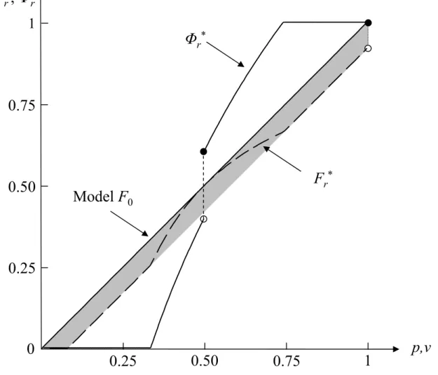
We now illustrate the equilibrium behavior with the uniform model distribution:
F0(v) =v;
where the pro…t maximizing pricep0 under the model distribution is given by p0 = 12:We
graphically represent the optimal behavior of the seller and nature for a small neighborhood.
The interior curve in the above graph identi…es the model distribution. Constraints induced by small changes in values cause the distribution function of Fr to be within an" bandwidth of the model distribution. The large changes of values, occurring with probability of at most"move the smallest valuation to the largest valuation, namely1. The strategy of nature is then to place as little probability as necessary below the range of the prices o¤ered by the seller and to shift values above the range as high as possible. Inside the range of prices o¤ered by the seller, nature uses a density function which maintains the virtual utility of the seller at0. In turn, the seller sets the density to make nature indi¤erent between all values above the mass point and all values below the mass point. Given the mass point set by the seller, nature shifts as much mass as possible below this point. We observe that even with the small neighborhood of "= 0:04, the impact of the ambiguity on the probabilistic price is rather large and leads to a wide spread in the prices o¤ered by the seller.
It remains to describe the comparative static of the probabilistic price and the regret of the seller as a function of the size of the neighborhood. The behavior of regret and the expected price to a marginal increase in ambiguity can be explained by the …rst order e¤ects. For a small level of ambiguity, we may represent the regret through a linear approximation
r =r0+"
@r @",
wherer0is the regret at the model distribution. For a small level of ambiguity, the marginal
change in regret can then be computed by holding the probabilistic price of the seller at the optimal price p0 without ambiguity. Suppose then for the moment that p0 12: If the
ambiguity increases marginally, the constraints on the choice of a least favorable demand are relaxed. What precisely then can nature do given the speci…cation of neighborhood. First nature can place the density f0(p0) slightly below p0 to marginally increase regret
by p0f0(p0), then nature can shift each value up by " to marginally increase regret by 1
and …nally shift mass from 0 to 1 to marginally increase regret by 1 p0: The …rst two
changes correspond to small changes in valuation with large probability, the third to large changes in the valuation with small probability. So the overall marginal e¤ect on regret of an increase in "near"= 0 is:
p0f0(p0) + 1 + (1 p0):
If instead the optimal price without ambiguity would bep0 > 12, then the only modi…cation
would a¤ect the third element as nature would move mass from0to just below p0, so that
the marginal increase would be
The optimal response of the seller to an increase in ambiguity is now to …nd a probabilistic price which minimizes the additional regret
"@r @"
coming from the increase in ambiguity. Of course, the cost of adjusting the price to minimize the marginal regret is that it changes the regret relative to the model distribution F0.
Locally, the cost of moving the price away from the optimum is given by the second derivative of the objective function. With small ambiguity, the curvature of the regret is identical to the curvature of the pro…t function. The rate at which the minimax regret price responses to an increase in ambiguity is then simply the ratio of the response of the marginal regret to a change in price divided by the curvature of the pro…t function, or
@E @" [pr] = @ @p @r @" @2 (@p)2 (p0; F0) .
The next proposition shows that the above intuition can be made precise and shows its implication for the net utility of the buyer.
Proposition 6 (Comparative Statics with Minimax Regret)
The expected price E[pr] responds to an increase in ambiguity at"= 0 by: @ @" E[pr]j"=0= 8 < : 1 f0(p0)+1 @ 2(p 0;F0)=@p2 1 if p0 1 2 1 f0(p0) 1 @ 2(p 0;F0)=@p2 1 2 if p0> 1 2 . (5)
We observe that for p0 > 12, the response of the expected price E[pr]to an increase in ambiguity is identical under regret minimization and pro…t maximization. The di¤erence arises at a low level of p0 at which the seller is less aggressive in lowering her price due to
an increase in ambiguity. As an implication from Proposition 6, we …nd that in the class of linear densities the change in expected price as well as the change in the mass point is strictly positive if and only if the density is strictly decreasing. This has to be contrasted with the maximin behavior where any increase in size of the ambiguity has a downward e¤ect on prices for all model distributions.
4.2 Menu Pricing
So far, our analysis assumed that the seller can only o¤er an indivisible object at some price p. We now extend the instruments of the seller and allow her to o¤er a menu of items. The
equilibrium policies with menus rather than single prices can be directly derived from the random pricing policies studied earlier and thus little new analysis will be necessary. The equilibrium use of menus allows us to understand the selling policies from a di¤erent and perhaps more intuitive point of view. The optimality of menus also emphasizes the role of robustness concerns in the optimal selling policies as menus would never be used in the standard setting for a given demand distribution.
If the allocative decision regards an indivisible object, orx2 f0;1g, then a speci…c item on the menu assigns a probability of receiving the object at a corresponding price. If on the other hand, the allocative decision regards a continuous variable, orx2[0;1], then a menu o¤ers a variety of quantities at di¤erent prices. We observe that with the multiplicative utility v x used here, the notions of probability and quantity are mathematically inter-changeable. In a direct mechanism, a menu is a pair (x(v); p(v)) which maps a reported typevinto a quantityx(v)and pricep(v). We transform an equilibrium probabilistic price into a menu policy by de…ning the quantity assigned in the direct mechanism through:
xr(v), r(v); (6)
and the corresponding nonlinear prices as:
pr(v),
Z v
0
yd r(y): (7)
By standard arguments recorded in Lemma 2 in the appendix this assignment of quantities to values de…nes an incentive compatible mechanism.
Form the point of view of menus, the minimax regret menu o¤ered by seller then has three important characteristics. These properties can be described with reference to the mass point b: (i) low volume o¤ers are made for buyers with low valuations, or v < b,
(ii) a much higher o¤er is made for all buyers with valuation v =b, and (iii) even higher volume o¤ers are made to buyers with large valuesv > b. We may think of a standard o¤er given by the quantity o¤ered at v = b, and given by x (b). In addition, the seller o¤ers low volume downgrades and high volume upgrades. The expanded menu relative to the optimal single item menu for the model distribution seeks to minimize the exposure of the seller. Obviously, the seller looses pro…ts on the high value buyers from making o¤ers to the low value buyers by granting the high value buyers a larger information rent. The size of the information rent is kept small by o¤ering menu items to the low value buyers only of substantially lower volume. This is the source of the gap in the quantities o¤ered in the menu.
A natural comparison to a minimax regret decision maker is a risk averse decision maker. In particular, we could ask how the behavior of a risk averse seller would di¤er from the behavior of a minimax regret seller. Clearly, a risk averse seller would never …nd a probabilistic price optimal. However, if she can o¤er lotteries or if the good is divisible then a risk averse seller might indeed o¤er a menu. The menu would consist of a set of possible quantity and price combinations. The di¤erence with respect to the minimax regret seller would then be in the shape of the menu. In particular, if a risk averse seller were to face a continuous demand function (as expressed byF0), then the optimal menu can be
shown to be continuous. Yet, with a minimax regret seller, we saw that the optimal menu is discontinuous (at a single jump point) and essentially o¤ers two (or three) classes of distinct service.
The minimax regret problems with ambiguity then o¤ers an interesting and novel reason for menus. Despite the prevalence of menus, the literature currently o¤ers only two leading explanations for menus in the standard monopoly setting: menus can be optimal if the marginal willingness to pay changes with the quantity o¤ered as in Deneckere & McAfee (1996) or if the buyers are budget constrained as in Che & Gale (2000).
The minimax regret response of the seller to an increase in ambiguity is perhaps even more informative when we consider menus. In a menu, the seller is o¤ering many di¤erent choices to the buyers. An immediate question therefore is how the choice set for the buyers changes with an increase in the ambiguity. We de…ne the size of the menu simply as the range of quantities o¤ered by the seller (and accepted by some buyers) in equilibrium.
Proposition 7 (Menus and Ambiguity)
For small ambiguity:
1. The size of the menu is increasing in ":
2. The price per unit pr(v)=xr(v) is decreasing in ".
As the ambiguity increases, the seller seeks to minimize her exposure by o¤ering more choices to the buyers and hence increasing the probability of a sale, even if the sale is not “big” in terms of the sold quantity. For every given valuation v, the seller also increases the size of the deal o¤ered. As larger deals are o¤ered to buyers with lower valuations, it follows that the seller is willing to concede a larger information rent to buyers with higher valuations. In consequence, the average price per unit is decreasing as well. Jointly, these three properties imply that the seller is o¤ering her products more aggressively and to a
larger number of buyers with an increase in ambiguity. We observe that the monotonicity in the unit price holds even as the previous proposition showed that the expected price may be increasing. The resolution of this apparent con‡ict comes from the fact that the seller is o¤ering larger quantities in response to an increase an ambiguity.
4.3 Robustness
We conclude this section by showing that the solution to the minimax regret problem also generates a robust policy in the sense of De…nition 1.
Proposition 8 (Robustness)
If r attains minimax regret at F0 for all su¢ ciently small "then f "rg is robust at F0:
5
Conclusion
In this paper we analyzed robust pricing policies by a monopolist. We introduced robustness by allowing for multiple priors in the neighborhood of a model distribution. We analyzed the optimal pricing of a monopolist under two distinct, but related decision criteria with multiple priors: maximin pro…t and minimax regret. We showed that the solution under either criterion yields a robust solution in the statistical sense. The expected revenue under either pricing rule is arbitrarily close to the optimal price for any distribution in a su¢ ciently small neighborhood of the model distribution. Despite the common robustness property, the prices respond di¤erently to the ambiguity. The maximin policy uniformly maintains a deterministic price policy and uniformly lowers the price by an increase in ambiguity. In contrast, the minimax policy balances the downside versus the upside when responding to the ambiguity. Here the trade-o¤ is optimally resolved by a probabilistic price. Importantly, the expected price does not necessarily decrease with an increase in ambiguity. Interestingly, an equivalent policy to the probabilistic price is achieved by a menu. The menu o¤ers a variety of quantities, ranging from small to large quantities to the buyer. By o¤ering a menu, the seller can guarantee himself small deals on the downside and large deals on the upside. In consequence, the seller hedges to reduce maximal regret by o¤ering multiple choices through a menu.
The problem of optimal monopoly pricing is in many respects the most elementary mechanism design problem. It would be of interest to extend the insights and apply the techniques developed here to a wide class of design problems, such as the discriminating monopolist (as in Mussa & Rosen (1978) and Maskin & Riley (1984)) and optimal auctions.
The monopoly setting has the simplifying feature that the buyers have complete information about their payo¤ environment. Given their known valuation and known price, each buyer simply had to make a decision as to whether or not to purchase the object. With the complete information by the buyer, there was no need to look for a robust purchasing rules. A substantial task would consequently arise by considering multi-agent design problems with incomplete information such as auctions, where it becomes desirable to “robustify”both the decisions of the buyers and the seller. The recent result by Segal (2003) and Chung & Ely (2003) regarding the su¢ cient conditions for the existence of dominant strategies for the bidders in optimal auctions might o¤er a …rst step in this direction. The complete solution of these problems poses a rich …eld for future research.
6
Appendix
The appendix contains some auxiliary results and the proofs for the results in the main body of the text.
Proof of Proposition 1. As shown in the text, if Fm is such that
Fm(v) = minfF0(v+") +";1g,
then (p; Fm) (p; F) for all F 2 P"(F0): On the other hand, if pm = p (Fm) then
(pm; Fm) (p; Fm)holds for allpby de…nition ofpm:Together this implies that(pm; Fm) is a saddle point as described in (SPm) and thus pm attains maximin payo¤ and Fm is a least favorable demand given pm.
Proof of Proposition 2. For su¢ ciently small"our assumptions onF0 imply thatFm is di¤erentiable near pm: Since pm is optimal given demand Fm we …nd that pm satis…es the associated …rst order conditions
d
dp(p(1 Fm(p)))jp=pm = 0:
The earlier concavity assumptions on F0 imply that we can apply the implicit function
theorem at "= 0 and this yields the statement to be proven.
Proof of Proposition 3. We show that for any > 0 there exists " > 0 such that F 2 P"(F0) implies (p (F); F) (pm; F) < : Note that (pm; F) (pm; Fm) and thus
(p (F); F) (pm; F) (p (F); F) (pm; Fm):
Since pm =p (Fm) the proof is complete once we show that (p (F); F) is a continuous function of F with respect to the Prohorov neighborhood. Consider F;Fbv such that Fbv 2 P"(F):Using the fact that
b
Fv(p) F(p+") +";
we obtain
p Fbv ;Fbv p (F) ";Fbv = (p (F) ") 1 Fbv(p (F) ")
(p (F) ") (1 F(p (F)) ") (p (F); F) 2":
Since the Prohorov norm is symmetric and thus F 2 P" Fbv , it follows that
and hence we have proven that (p (F); F) is continuous inF.
Proof of Proposition 4. We apply Corollary 5.2 in Reny (1999) to show that a saddle point exists. For this we need to verify that the zero-sum game between the seller and nature is a compact Hausdor¤ game for which the mixed extension is both reciprocally upper semi continuous and payo¤ secure.
Clearly we have a compact Hausdor¤ game. Reciprocal upper semi continuity follows directly as we are investigating a zero-sum game. So all we have to ensure is payo¤ security. Payo¤ security for the monopolist means that we have to show for each (Fr; r) with Fr 2 P"(F0) and for every > 0 that there exists > 0 and F such that F 2 P (Fr) implies r ; F r( r; Fr) + :
Let , =4 and let be such that (p) , r(p+ ): Then using the fact that F(v) Fr(v ) we obtain Z 1 0 vdF(v) 2 + Z 1 0 vdFr(v):
Using the fact that F(v) Fr(v+ ) + we obtain
; F ( r(p+ );minfFr(v+ ) + ;1g) ( r; Fr) 2 and hence
r ; F r( r; Fr) + :
To show payo¤ security for nature we have to show for each( r; Fr)withFr2 P"(F0) and
for every > 0 that there exists > 0 and F 2 P"(F0) such that 2 P ( r) implies r ; F r( r; Fr) :
Here we setF ,Fr:Given >0consider any 2 P ( r). All we have to show is that
( ; Fr) ( r; Fr) + for su¢ ciently small :Note that (p) r(p+ ) + implies
( ; Fr) + Z (p+ ) Z 1 p dFr(v) d r(p+ ) = + Z p Z 1 p dFr(v) d r(p) = + ( r; Fr) + Z p Z [p ;p) dFr(v) ! d r(p) + ( r; Fr) + Z Z [p ;p) dFr(v)d r(p): Given continuity of Z Z [p ;p) dFr(v)d r(p)
in the claim is established.
In order to derive the equilibrium policies in the case of small ambiguity we present a characterization of the Prohorov distance in Lemma 1 that builds on the following result of Strassen (1965).
Theorem (Strassen (1965)).
F andGhave Prohorov distance less than or equal to"if and only if there exist random vari-ablesXandY such thatXhas distributionF; Y has distributionGandPr (jY Xj ") 1 ".
The two cumulative distributionsF; Gare close if and only if they are associated to two random variables that realize similar values with high probability. Our characterization describes the Prohorov distance in terms of cumulative distribution functions only. In order to stay within " distance of a given distribution function G one may …rst alter any value by at most ", this creates a probability measure F1, and then move at most" mass of the
values. The new locations are described by a measureF2 while locations from where mass
has been taken is described by a measureF3.
Lemma 1 (Decomposition)
Consider " >0 and probability measures F and G. F 2 P"(G) if and only if there exists a probability measure F1 and positive additive measures F2 and F3 such that:
G(x ") F1(x) G(x+"); F2; F3 ";
and
F F1+F2 F3:
Proof. (() SupposeF can be decomposed into F1; F2 and F3. We want to show that
F(A) G(A") +". To this purpose, it is clearly su¢ cient su¢ cient to consider only closed setsA.
(a) We …rst prove the claim for A = [x; y] with 0 x y 1: Given a probability measure H let H (vb),limv"bvH(v):Then
F1([x; y]) =F1(y) F1 (x) G(y+") G (x ") =G([x; y]"):
Since F2([x; y]) "and F3([x; y]) 0 we obtain:
(b) Next we consider A= [x1; y1][[x2; y2]withy1+ 2" < x2 which implies that [x1; y1]"\[x2; y2]"=;:
Using part (a) together with the fact thatA" = [x1; y1]"[[x2; y2]"holds for the[ ]"operator,
it follows that:
F1(A) =F1([x1; y1]) +F1([x2; y2]) G([x1; y1]") +G([x2; y2]") =G(A"):
Since F2(A) "and F3(A) 0, the claim is proven.
(c) The arguments in part (b) are easily generalized for any setAthat can be decomposed into a …nite union of disjoint closed intervals of distance greater than2"soA=[mk=1[xk; yk] withxk yk< xk+1+ 2"fork m 1:
(d) Finally we show that we do not have to prove the statement for more general setsA. Notice that ifA"1 =A"2; A1 A2 andF(A2) G(A"2) +"thenF(A1) G(A"1) +":So we
can restrict attention to proving the claim for closed setsAsuch that A"=A"1 and A A1
implies A=A1:Consider x; y2Asuch that x < y x+ 2": Then fA[[x; y]g"=A" and
hence[x; y] A:It follows that Abelongs to the class of sets investigated in part (c).
()) Consider probability measures F and G with kF Gk ": We extend G to
[ ";1 +"] such that G(x) = 0 for " x < 0 and G(x) = 1 for 1 < x 1 + ": Given the result of Strassen (1965), there exist random variablesX andY such thatX has distributionF; Y has distributionGand Pr (jY Xj ") 1 ".
LetZ1 be the random variable with cdfF1 such thatZ1,X ifjY Xj "andZ1 ,Y
ifjY Xj> ". Let"0 ,Pr (jY Xj> ") so"0 ": Then G(x ") F1(x) G(x+"):
LetZ2 be the random variable with cdfFb2 such that Z2 ,0 ifjY Xj "and Z2 ,X if
jY Xj> ": LetZ3 be the random variable with cdf Fb3 such that Z3 ,0 if jY Xj "
and Z3 , Y if jY Xj > ": Then X = Z1 +Z2 Z3 and Fb2(0);Fb3(0) 1 "0: Let
Fi,Fbi (1 "0)fori= 2;3:ThenF2 andF3are positive additive measures withF2; F3 "0
and the proof is complete.
Proof of Proposition 5. We start by assumingp0 > 12:The proof proceeds in three steps.
First we show the existence of the parametersa; bandcand use these to construct the least favorable demand Fr: Second, we decompose the least favorable demand by using Lemma 1 to show that it is close to F0: Third we use this decomposition to verify that we have a
saddle point.
such thata < b < c and a < p0< c such that F0(a ") " = 1 b2f0(b+") a ; (8) F0(b+") = 1 b2f0(b+") b ; (9) F0(c ") = 1 b2f 0(b+") c : (10)
With respect to the existence of b;note that b=p0 solves (9) if "= 0. As
d
db(1 F0(b+") bf0(b+"))j"=0 = 2f(p0) p0(f0) 0(p
0)<0;
due to the strict concavity of pro…ts at p0, the implicit function theorem implies that a
solutionb=b(")to (9) (withb >0) exists for"in a neighborhood of 0. To prove existence of c;de…ne h(v),1 b 2f 0(b+") v F0(v ") forv >0: Then h(b) =F0(b+") F0(b ")with h0(b) =f0(b+") f0(b "); and h00(b) = 2f0(b+") b (f0) 0(b ") 2f0(p0) +p0(f0)0(p0) p0 <0:
We note that h(b) >0 by our earlier concavity assumptions onF0:Looking at the Taylor
approximation of h near v = b for small " we obtain that there exists c > b such that h(c) = 0withc!p0as"!0:As for the existence ofa;analogous calculations forh(v) +"
show that there existsa < b such thath(a) +"= 0 witha!p0 as"!0:
We can describe the local behavior of the parameters a; b and c by appealing to the implicit function theorem. Since2f0(p0) +p0(f0)0(p0)>0we know that bis di¤erentiable
and by implicitly di¤erentiating (9) we obtain:
b0(0) = f0(p0) +p0(f0) 0(p 0) 2f0(p0) +p0(f0)0(p0) = 1 + f0(p0) 2f0(p0) +p0(f0)0(p0) (11)
where 1 b0(0) 1=2:Next we show thatais di¤erentiable. Since b2f0(b+") a2f0(a ")
b a = (b+a)f0(b+") +a
2f0(b+") f0(a ")
b a
we …nd thatb2f0(b+")> a2f0(a ")near"= 0. Hence we can implicitly di¤erentiate (8) to obtain a0(") = aa+af0(a ") +bf0(b+") b2f 0(b+") a2f0(a ") ; (12) so lim "!0 b a a a 0(") = 1 + 2f0(p0) 2f0(p0) +p0(f0)0(p0) :
In particular we obtain that
lim
"!0a
0(") = 1: (13)
Similarly for c, we …nd that:
c0(") = c cf0(c ") +bf0(b+") b2f 0(b+") c2f0(c ") ; (14) and hence lim "!0 c b c c 0(") = 2f0(p0) 2f0(p0) +p0(f0)0(p0) ; and in particular, lim "!0c 0(") =1: (15)
It now follows from (13) and (15) that a < p0 < c.
Step 2. We now construct the least favorable demand on the basis of a; b and c. ConsiderFr given by Fr(v), 8 > > > > > < > > > > > : maxf0; F0(v ") "g, if v2[0; a] 1 b2f0(b+") v , if v 2(a; c) F0(v "), if v2[c;1) 1 if v= 1 ,
where the de…nitions of a and cimply that Fr is continuous at aand c. It follows that Fr is a probability measure.
Next we show thatFr2 P"(F0)by using Lemma 1. Consider F1 de…ned by
F1(v), 8 > > < > > : F0(v "), if v2[0; a] maxfFr(v); F0(v ")g, if v2(a; b) Fr(v); if v2[b;1] .
Then F1 is a probability measure with F0(v ") F1(v): By de…nition of b we obtain
Fr(b) =F0(b+") andFr0(b) = dvdF0(v+")jv=b:Moreover, givenFr00(v) =
2b2f 0(b+")
v3 and
d2
forv 2[a; c]and " su¢ ciently small. Thus, for su¢ ciently small"; as aand c are close to p0;we obtainF1(v) F0(v+")with equality ifv=b:So F0(v ") F1(v) F0(v+").
Consider F2 de…ned by:
F2(v), 8 > > < > > : 0, if v2[0; a] " maxfF0(v ") Fr(v);0g, if v2(a; b] "; if v2(b;1] . Then d dv (Fr(v) F0(v+")) = b2f0(b+") v2 f0(v+") 0 for v b; as d dv v 2f 0(v+") =v2(f0)0(v+") + 2vf0(v+")>0;
holds for "su¢ ciently small and henceF2 is weakly increasing withF2(1) =":Since F2 is
also right continuous we obtain that F2 is an additive probability measure.
Let F3 be de…ned by
F3(v),minfF0(v "); "g; ifv2[0;1];
so F3(v) is an additive probability measure and F3(1) = ": Since Fr = F1+F2 F3 we
obtain from Lemma 1 thatFr2 P"(F0):
Step 3. Next we show that (Gr; Fr) is a saddle point. For the monopolist we verify easily that (p; Fr) = b2f0(b+") for p 2 [a; c]: Similar to the calculations following the
de…nition ofF1it is easily shown that there exists >0such that1 b
2f 0(b+")
v < Fr(v)holds for all v 2 [p0 ; p0+ ]n[a; c] and all su¢ ciently small ": Thus, for su¢ ciently small "
we obtain[a; c] = arg maxp2[p0 ;p0+ ] (p; Fr) and together with the upperhemicontinuity
of pro…ts that[a; c] arg maxp (p; Fr).
Consider now the incentives of nature. Note that
r(Gr; Fr) =r(Gr; F1) +r(Gr; F2) r(Gr; F3); (16)
where we choose F2 and F3 such that F2(1) = F3(1) = ": In the following we show that
each term in (16) is maximized separately: If nature could put all mass on a single value v, by construction of Fr nature would be indi¤erent over v 2 [a; b) and over v 2 [b; c]: Sincer(Gr; v)is monotone increasing on[0; a]and[c;1]it follows thatarg maxvr(Gr; v)
[a; b)[ f1g:For su¢ ciently small "; r(Gr; a) p0 while r(Gr;1) 1 p0 and thus given
ConcerningF3letv= inffv:F0(v ") "g:We have to show thatr(Gr;ev) r(Gr;bv) for ve v bv: Given the above it is su¢ cient to consider only ve = v and bv = c where r(Gr; c) =c E(pr):Let ,2 supv>0F0v(v). For v su¢ ciently small,
v
F0(v) and hence
r(Gr;ev) =ve "+ F0(ev ") ="(1 + ): On the other hand, we showed in Step 1 that
@
@"cj"=0 = 1 and in the proof of Proposition 6 based only on arguments in Step 1 that @
@"E(pr)j"=0 < 1 so @
@"r(Gr; c)j"=0 = 1. Hence, r(Gr;ev) < r(Gr; c) for " su¢ ciently small.
Finally, considerF1:More mass cannot be allocated to regret maximizing values[a; b)as
F1(b) =F0(b+");weight on values belowaand abovecare shifted up as far as possible as
Fv(v) =F0(v ")forv < aandc < v <1and allocation ofF1 forF1 2(F1(b); F0(c "))
will not in‡uence regret as r(Gr; v) is constant on[b; c]:
The case ofp0 12 proceeds in an analogous manner. It is easily shown that there exist
parameters a; b; csuch that a < b < c anda < p0 < c such that
F0(a ") " = 1 b2f0(b+") a ; F0(b+") = 1 b2f 0(b+") b +"; (17) F0(c ") " = 1 b2f 0(b+") c ; where b0(0) = f0(0) +p0f 0 0(0) 1 2f0(0) +p0f00(0) = 1 + f0(0) + 1 2f0(0) +p0f00(0) :
The least favorable demand Fr is now given by:
Fr(v), 8 > > > > > < > > > > > : maxf0; F0(v ") "g, if v2[0; a] 1 b2f0(b+") v , if v 2(a; c) maxf0; F0(v ") "g, if v2[c;1) 1 if v= 1 , decomposed as Fr=F1+F2 F3 where F1(v), 8 > > > > > < > > > > > : F0(v "), if v2[0; a] 1 b2f0(b+") v +", if v2(a; c) F0(v "); if v2[c;1) 1 if v= 1 , F2(v), ( 0, if v2[0;1) ", if v= 1 ,
F3(v),minfF0(v "); "g; ifv2[0;1]:
Lemma 1 can be applied to show that Fr 2 P"(F0): In contrast to the previous case of
p0 > 12, now v = 1 maximizes r(Gr; v) so that F2 puts all mass at v = 1: For the case
of p0 = 12 Proposition 6 can be used to show that r(Gr;1) = 1 E[pr] > r(Gr; a) = a. As in the case where p0 > 12; F1(v) F0(v+") with tangency only at v= b soF1 again
maximizes weight on[a; b). [a; b) is now only a local maximum ofr(Gr; v) but nevertheless it still follows easily thatF1 maximizes regret (use the fact thatF0(b+")< F0(c ")).
Proof of Proposition 6. We obtain that
E[pr] = Z c a p1 pdp+b 1 Z c a 1 pdp =c a+b 1 ln c a :
Asa; b; and care di¤erentiable as shown in Step 1 of Proposition 5, we have: @ @"E[pr] = b a a a 0(") +c b c c 0(") + 1 lnc a b 0("):
Inserting the value fora0("); b0(")andc0(")from (11), (12) and (14) respectively, we obtain forp0 > 12 : @ @"E[pr]j"=0 = 1 + f0(p0) 1 2f0(p0) +p0(f0)0(p0) :
The same operations yield the result for p0< 12.
Proof of Proposition 7. Following Proposition 5,lim"!0a0(") = 1andlim"!0c0(") =
1and therefore the size of menu is increasing in"for"su¢ ciently small which proves (1). Next we verify (2). Assume a < v < b. Then x (v) = lnva and p (v) =Ravy1ydy=v aso given a0 <0 for"small we obtain @"@x (v)>0; @"@p (v)>0 and
@ @" p (v) x (v) = (v a)1a lnva lnva 2 a 0(")<0
as dvd (v a)a1 lnva = 1a 1v >0. Thus,x (v)v p (v) is strictly increasing in": Assumeb < v < c. Thenx (v) = 1 lncv andp (v) =v a+ 1 lnca b=E[pr]+v c so @"@x (v)<0; @"@p (v)<0 and @ @" p (v) x (v) = @ @"E[pr] 1 lnvc + 1 c (E[pr] +v c) 1 ln c v 1 lncv 2 c 0(")<0
where we use the fact thatc0(")is large and dvd 1c (E[pr] +v c) 1 lncv = 1c 1v <0 for"small. We obtain @ @"u(v) = v p (v) x (v) @ @"x (v) x (v) @ @" p (v) x (v) = c v c c 0(") @ @"E[pr]: Since incentive compatibility implies that x (v)v p (v) is continuous in v and since x has an upwards jump at v=b we obtain
p (b)
x (b) >vlim!b p (v)
x (v):
Clearly, xp ((vv)) > xp ((bb)) forv > bholds from above using right continuity ofx .
The following lemma shows how probabilistic prices can be transformed into menus and vice versa.
Lemma 2 (Equivalence)
1. For any mixed pricing policy (v) the menu (x(v); p(v))is incentive compatible.
2. If(x(v); p(v))is incentive compatible, then there exists a mixed pricing policy such that ( ; v) p(v) for all v2[0;1]:
Proof. First we show that if g: [0;1]![0;1]is non decreasing then vg(v) Z v 0 sdg(s) Z v 0 g(s)ds 0:
Lethbe the left hand side of this equation. Clearly,h(0) = 0. Sincegis non decreasing and bounded,his di¤erentiable almost everywhere which implies thath0 = 0almost everywhere. Consider somev2[0;1]:Ifgis continuous atvthen so ish:Assume thatgis not continuous atv: Then vg(v) Z v 0 sdg(s) = lim v"vvg(v)+v g(v) limv"vg(v) limv"v Z v 0 sdg(s) v g(v) lim v<!vg(v) soh is continuous atv and thus h 0.
For the rest of the proof we can use a standard result on incentive compatibility, see Proposition 23.D.2 in Mas-Collel, Whinston & Green (1995). Part (1) follows immediately from the fact that Fp is nondecreasing and that v (v) ( ; v) =
Rv
0 (s)ds given our
For part (2), notice that x(v) 2 [0;1] and that incentive compatibility implies that x(v) is non decreasing and vx(v) p(v) = R0vx(s)ds. Moreover, we can limit attention to menus where xis right continuous as otherwise there exists a right continuous incentive compatible menu (xb(v);pb(v))v2[0;1] such thatpb(v) p(v) for all v:As we considerx that is right continuous, such that (v) , x(v) for all v is a well de…ned mixed pricing policy and we obtain p(v) = vx(v) R0vx(s)ds. Our calculations above then imply that
( ; v) =p(v):
Proof of Proposition 8. Assume that pbattains minimax regret but is not robust. So there exists >0 such that for all" >0 there existsF" such thatF"2 P"(F0) but
(p (F"); F") (pb(F0; "); F") : (18) Assume that(pb(F0; "); G")is a saddle point of the regret problem (SPr) given" >0. Then
r(pb(F0; "); G") = sup F2P"(F0) r(bp(F0; "); F); and hence b p(F0; ") =p (G"):
We can rewrite the left hand side of (18) as follows:
(p (F"); F") (pb(F0; "); F") (19)
= (p (F"); F") (p (G"); G") + (p (G"); G") (p (G"); F"):
Using (SPr) we also obtain
0 r(p (G"); G") r(p (G"); F") = Z vdG"(v) Z vdF"(v)+ (p (G"); F") (p (G"); G") so that: (p (G"); G") (p (G"); F") Z vdG"(v) Z vdF"(v):
Entering this into (19) we obtain from (18) that:
(p (F"); F") (p (G"); G") +
Z
vdG"(v)
Z
vdF"(v) : (20)
Since F"; G"2 P"(F0) and since h(v) =v is a continuous function and the Prohorov norm
metricizes the weak topology we obtain that
Z
vdG"(v)
Z
if"is su¢ ciently small.
In the proof of Proposition 3 we showed that (p (F); F)as a function ofF is contin-uous with respect to the Prohorov neighborhood. Hence
(p (F"); F") (p (G"); G")< =2 (22)
References
Anscome, F.J. & R.J. Aumann. 1963. “A De…nition of Subjective Probability.”Annals of Mathematical Statistics34:199–205.
Bell, D.E. 1982. “Regret in Decision Making under Uncertainty.”Operations Research 30:961–981.
Bose, S., E. Ozdenoren & A. Pape. 2006. “Optimal Auctions with Ambiguity.”Theoretical Economics1:411–438.
Che, Y.K. & I. Gale. 2000. “The Optimal Mechanism for Selling to a Budget Constrained Buyer.”Journal of Economic Theory 92:198–233.
Chung, K.-S. & J. Ely. 2003. “Implementation with Near-Complete Information.” Econo-metrica71:857–871.
Deneckere, R.J. & R.P. McAfee. 1996. “Damaged Goods.”Journal of Economics and Man-agement Strategy5:149–174.
Ellsberg, D. 1961. “Risk, Ambiguity and the Savage Axioms.”Quarterly Journal of Eco-nomics75:643–669.
Engelbrecht-Wiggans, R. 1989. “The E¤ect of Regret on Optimal Bidding in Auctions.” Management Science35:685–692.
Engelbrecht-Wiggans, R. & E. Katok. 2007. “Regret in Auctions: Theory and Evidence.” Economic Theoryp. forthcoming.
Filiz, E. & E.Y. Ozbay. 2006. Auctions with Anticipated Regret: Theory and Experiment. Technical report Columbia University and New York University.
Gilboa, I. & D. Schmeidler. 1989. “Maxmin Expected Utility with Non-Unique Prior.” Journal of Mathematical Economics18:141–153.
Hannan, J. 1957. Approximation to Bayes Risk in Repeated Play. In Contributions to the Theory of Games, ed. M. Dresher, A.W. Tucker & P. Wolfe. Princeton: Princeton University Press pp. 97–139.
Hansen, L. Peter & T. Sargent. 2004. Misspeci…cation in Recursive Macroeconomic Theory. Technical report University of Chicago, New York University, and Hoover Institution.
Harris, M. & A. Raviv. 1981. “A Theory of Monopoly Pricing Schemes with Demand Uncertainty.”American Economic Review71:347–365.
Hayashi, T. 2006. Regret Aversion and Opportunity Dependence. Technical report Univer-sity of Texas.
Huber, P.J. 1964. “Robust Estimation of a Location Parameter.”Annals of Mathematical Statistics35:73–101.
Huber, P.J. 1965. “A Robust Version of the Probability Ratio Test.”Annals of Mathematical Statistics36:1753–1758.
Klibano¤, P., M.Marinacci & S. Mukerji. 2005. “A Smooth Model of Decision-Making under Ambiguity.”Econometrica73:1849–1892.
Linhart, P.B & R. Radner. 1989. “Minimax - Regret Strategies for Bargaining over Several Variables.”Journal of Economic Theory 48:152–178.
Loomes, G. & R. Sugden. 1982. “Regret Theory: An Alternative Theory of Rational Choice under Uncertainty.”Economic Journal 92:805–824.
Lopomo, G., L. Rigotti & C. Shannon. 2006. Uncertainty in Mechanism Design. Technical report.
Mas-Collel, A., M.D. Whinston & J.R. Green. 1995.Microeconomic Theory. Oxford: Oxford University Press.
Maskin, E. & J. Riley. 1984. “Monopoly with Incomplete Information.”Rand Journal of Economics15:171–196.
Milnor, J. 1954. Games Against Nature. In Decision Processes, ed. R.M. Thrall, C.H. Coombs & R.L. Davis. New York: Wiley.
Mussa, M. & S. Rosen. 1978. “Monopoly and Product Quality.”Journal of Economic Theory18:301–317.
Neumann, J. Von & O. Morgenstern. 1953. Theory of Games and Economic Behavior. Princeton: Princeton University Press.
Prasad, K. 2003. “Non-Robustness of some Economic Models.”Topics in Theoretical Eco-nomics3:1–7.