Quantification of Prediction Uncertainty for Principal Components Regression and Partial Least Squares Regression

(1)

Principal Components Regression and Partial

Least Squares Regression

by

Ying Zhang

A Thesis Submitted for the Degree of

Doctor of Philosophy

in the

Faculty of Mathematical & Physical Sciences

Department of Statical Science

(2)

Declaration of Authorship

I,

, confirm that the work

pre-sented in this thesis is my own. Where information has

been derived from other sources, I confirm that this has

been indicated in the thesis.

(3)

Principal components regression (PCR) and partial least squares regression (PLS) are widely used in multivariate calibration in the fields of chemometrics, economet-rics, social science and so forth, serving as alternative solutions to the problems which arise in ordinary least squares regression when explanatory variables are either collinear, or there are hundreds of explanatory variables with a relatively small sample size. Both PCR and PLS tackle the problems by constructing lower dimensional factors based on the explanatory variables.

The extra step of factor construction makes the standard prediction uncer-tainty theory of ordinary least squares regression not directly applicable to the two reduced dimension methods. In the thesis, we start by reviewing the ordi-nary least squares regression prediction uncertainty theory, and then investigate how the theory performs when it extends to PCR and PLS, aiming at potentially better approaches.

The first main contribution of the thesis is to clarify the quantification of pre-diction uncertainty for PLS. We rephrase existing methods with consistent math-ematical notations in the hope of giving a clear guidance to practitioners.

The second main contribution is to develop a new linearisation method for PLS. After establishing the theory, simulation and real data studies have been employed to understand and compare the new method with several commonly used methods. From the studies of simulations and a real dataset, we investigate the prop-erties of simple approaches based on the theory of ordinary least squares theory, the approaches using resampling of data, and the local linearisation approaches including a classical and our improved new methods. It is advisable to use the ordinary least squares type prediction variance with the estimated regression error variance from the tuning set in both PCR and PLS in practice.

(4)

Acknowledgements

First and foremost, I would like to thank my primary supervisor, Professor Thomas Fearn. I am greatly indebted to him, for sharing his intellect with me, his highly professional guidance, and his patience to read my reports and drafts. I feel very fortunate to have had the opportunity to study with him. I would like to thank my parents, Qingping Zhang and Pu Wang, for their generous support and encouragement. They are my best friends in life. Without them, I would not have been able to pursue my interests. I am very thankful to my secondary supervisor, Dr. Jinghao Xue, for his kind suggestions about my upgrade report and my PhD research life.

I would like to express sincere gratitude to the department of Statistical Science and its staff. I am especially grateful to my MSc advisor, Dr. Rex Galbraith, for opening the door of Statistics for me. I greatly appreciate the guidance from my MSc research project supervisors, Professor Richard Chandler and Dr. Afzal Siddiqui. I would like to thank Ms. Marion Ware and Dr. Ying Zhu for their help and advice on my applications to the MSc and PhD programs.

I would like to thank Goodenough College for providing me a comfortable home in London. I would also like to thank my friends, for accompanying me during the PhD study.

(5)

1 Introduction 14

1.1 Multiple Linear Regression and Prediction Uncertainty . . . 15

1.2 Principal Components Regression (PCR) and Partial Least Squares Regression (PLS) . . . 18

1.3 The Problem of Prediction Uncertainty . . . 19

1.4 Notation . . . 23

2 OLS Prediction Uncertainty 25 2.1 Ordinary Least Squares Regression Theory . . . 26

2.2 Ordinary Least Squares Regression Simulation Study . . . 27

2.2.1 Methodology . . . 27

2.2.2 Ordinary Least Squares Prediction Uncertainty Simulation . 28 2.2.3 The Use of a Tuning Set . . . 39

2.2.4 Cross-validation . . . 43

2.2.5 Random Data Splitting . . . 44

2.3 Some Comments on Leverage . . . 48

2.4 Summary . . . 49

3 PCR Prediction Uncertainty 50 3.1 Principal Components Regression Theory . . . 51

3.1.1 Principal Components . . . 51

3.1.2 Singular Value Decomposition . . . 52

3.1.3 Principal Components Regression . . . 53

3.2 Principal Components Regression Prediction Uncertainty . . . 55

3.2.1 Simple Empirical Estimates: RMSEP and RMSECV . . . . 56

3.2.2 Ordinary Least Squares Type Prediction Mean Squared Error 56 3.3 Principal Components Regression Simulation Study . . . 57

(6)

Contents

3.3.2 Bias and PCR Prediction Uncertainty . . . 61

3.3.3 Sample Size and PCR Prediction Uncertainty . . . 71

3.3.4 Correlation between Leverage and Bias . . . 72

3.4 Summary . . . 79

4 PLS Prediction Uncertainty 80 4.1 Partial Least Squares Regression Algorithms . . . 80

4.1.1 Orthogonal Scores Algorithms . . . 81

4.1.2 Orthogonal Loadings Algorithms . . . 86

4.2 PLS Prediction Uncertainty Literature Review . . . 88

4.2.1 Simple Empirical Estimates: RMSEP and RMSECV . . . . 88

4.2.2 Ordinary Least Squares Type Mean Squared Error . . . 89

4.2.3 Linearisation Based Methods . . . 90

4.2.4 Re-sampling Methods . . . 92

4.2.5 U-deviation Methods . . . 95

4.2.6 Regression Error Variance Estimates and Degrees of Freedom 97 4.3 Summary . . . 99

4.4 Appendix . . . 99

5 A Modified PLS Linearisation Method 101 5.1 Background . . . 102

5.2 New Linearisation Method Theory . . . 105

5.2.1 The Asymptotic Distribution of Var (b0) . . . 106

5.2.2 ∂qˆ/∂b . . . 106

5.2.3 ∂wlR˜/∂b . . . 109

5.3 New Linearisation Method Bootstrapping Estimate . . . 110

5.4 Univariate PLS Prediction Mean Squared Error Summary . . . 111

5.5 Univariate Partial Least Squares Regression Simulation Study . . . 116

5.5.1 PLS Simulation with Noise Free Prediction Samples . . . 119

5.5.2 PLS Simulation Using the Estimated Regression Error Vari-ance from the Calibration Set . . . 140

(7)

5.5.3 PLS Simulation Including the Error Term in Prediction

Sam-ples . . . 145

5.6 An Example of Real Data Analysis . . . 148

5.6.1 Silage Data Analysis . . . 148

5.6.2 PLS Random Data Splitting Simulation in Imitation of the Silage Data . . . 155

5.6.3 PLS Simple Random Data Splitting Simulations . . . 158

5.7 Summary . . . 164 5.8 Appendix . . . 166 5.8.1 ∂Siwi/∂vecut(Si) . . . 166 5.8.2 ∂w′ iSiwi/∂vecut(Si) . . . 166 5.8.3 ∂vecut(uiu′i)/∂ui . . . 167 6 Conclusions 168 6.1 Ordinary Least Squares Regression Prediction Uncertainty Study Summary . . . 168

6.2 Principal Components Regression Prediction Uncertainty Study Sum-mary . . . 170

6.3 Partial Least Squares Regression Prediction Uncertainty Study Sum-mary . . . 171

6.4 Conclusions . . . 172

(8)

List of Figures

2.1 OLS Average Squared Prediction Error versus Average Leverage, i.i.d. standard normally distributed predictors . . . 31 2.1 OLS Average Squared Prediction Error versus Average Leverage,

i.i.d. standard normally distributed predictors . . . 32 2.2 OLS Average Squared Prediction Error versus Average Leverage,

uniformly distributed leverage. . . 36 2.3 OLS Average Squared Prediction Error versus Average Leverage,

uniformly distributed leverage, three different simulations of yc for

a fixed Xc. . . 38

2.3 OLS Average Squared Prediction Error versus Average Leverage, uniformly distributed leverage, three different simulations of yc for

a fixed Xc (cont.) . . . 39

2.4 OLS Squared Prediction Error versus Leverage in a Tuning Set, i.i.d. standard normally distributed predictors, one ( ˙Xc,y˙c). . . 42

2.5 OLS Average Squared Prediction Error versus Average Leverage for One Set of Simulated Data, random data splitting, ξ_p = 0.25. . . . 46 2.6 OLS Average Squared Prediction Error versus Average Leverage for

400,000 Sets of Simulated Data, random data splitting . . . 47 3.1 PCR Histogram: the Number of Principal Components . . . 60 3.2 PCR Average Squared Prediction Error versus Average Leverage,

i.i.d. standard normally distributed predictors, ǫp =0 . . . 62

3.3 PCR Average Squared Prediction Error versus Average Leverage, to verify the missing part of the ordinary least squares type prediction mean squared error is the expected squared bias, ǫp 6=0. . . 66

(9)

3.4 PCR Average Squared Prediction Error versus Average Leverage, i.i.d. standard normally distributed predictors, ǫp = 0, adjusted

ordinary least squares type prediction mean squared error. . . 68 3.5 PCR Average Squared Prediction Error versus Average Leverage,

i.i.d. standard normally distributed predictors, ǫp 6= 0, adjusted

ordinary least squares type prediction mean squared error. . . 70 3.6 PCR the Relationship between Prediction Mean Squared Error and

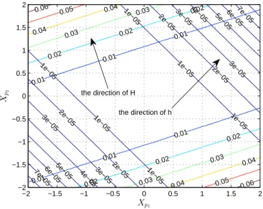
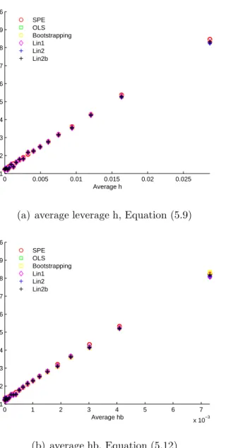
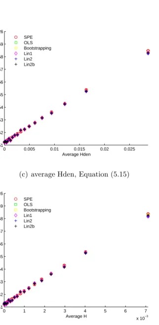
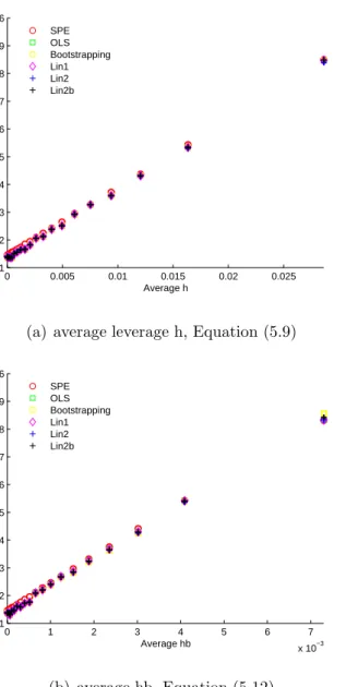
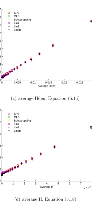
Sample Size. . . 73 3.7 PCR the Relationship between the Squared Bias and the Leverage . 77 5.1 PLS: a Contour Plot to Show the Directions of h and H . . . 115 5.2 PLS Average Squared Prediction Error versus Average Distance

Measure. k =a = 1, Var ( ˙Xc) = 1, σǫ2 = 0.25, ǫp =0. . . 120

5.2 PLS Average Squared Prediction Error versus Average Distance Measure. k =a = 1, Var ( ˙Xc) = 1, σǫ2 = 0.25, ǫp =0 (cont.). . . 121

5.2 PLS Average Squared Prediction Error versus Average Distance Measure. k =a = 1, Var ( ˙Xc) = 1, σǫ2 = 0.25, ǫp =0 (cont.). . . 122

5.3 PLS Average Squared Prediction Error versus Average Distance Measure, k = 2, a= 1, Var ( ˙Xc1) = 25, Var ( ˙Xc2) = 1, β0 =β1 = 1,

β2 = 0, σǫ2 = 0.25, ǫp =0. . . 123

β2 = 0, σǫ2 = 0.25, ǫp =0 (cont.). . . 124

β2 = 0, σǫ2 = 0.25, ǫp =0 (cont.). . . 125

5.4 PLS ˆβ againstbwhen k= 2, a= 1, Var ( ˙Xc1) = 25, Var ( ˙Xc2) = 1,

β0 =β1 = 1, β2 = 0, σǫ2 = 0.25, ǫp =0. . . 125

5.5 PLS Average Squared Prediction Error versus Average Distance Measure. k = 2, a = 1, Var ( ˙Xc1) = 25, Var ( ˙Xc2) = 1, β1 = 0,

(10)

List of Figures 5.5 PLS Average Squared Prediction Error versus Average Distance

Measure. k = 2, a = 1, Var ( ˙Xc1) = 25, Var ( ˙Xc2) = 1, β1 = 0,

β0 =β2 = 1, σǫ2 = 0.25, ǫp =0 (cont.). . . 128

5.5 PLS Average Squared Prediction Error versus Average Distance Measure. k = 2, a = 1, Var ( ˙Xc1) = 25, Var ( ˙Xc2) = 1, β1 = 0,

β0 =β2 = 1, σǫ2 = 0.25, ǫp =0 (cont.). . . 129

5.6 PLS ˆβ againstbwhen k= 2, a= 1, Var ( ˙Xc1) = 25, Var ( ˙Xc2) = 1,

β1 = 0, β0 =β2 = 1 , σǫ2 = 0.25, ǫp =0. . . 129

5.7 PLS Average Squared Prediction Error versus Average Distance Measure. k = 3, a = 2, Var ( ˙Xc1) = Var ( ˙Xc2) = 25, Var ( ˙Xc3) = 1,

β1 =β2 = 1, β3 = 0, , σ2ǫ = 0.25, ǫp =0. . . 130

β1 =β2 = 1, β3 = 0, , σ2ǫ = 0.25, ǫp =0 (cont.). . . 131

β1 =β2 = 1, β3 = 0, , σ2ǫ = 0.25, ǫp =0 (cont.). . . 132

5.8 PLS Histograms for Six Selected Elements in Var ( ˆβ) Calculated by the New Linearisation Method in the Case when k = 3, a = 2, Var ( ˙Xc1) = Var ( ˙Xc2) = 25, Var ( ˙Xc3) = 1, β1 = β2 = 1, β3 = 0,

σ2

ǫ = 0.25, ǫp =0. . . 133

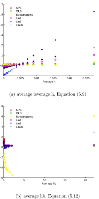
5.9 PLS Goodness of Fit for the New Linearisation Approximation in the Case when k = 3, a = 2, Var ( ˙Xc1) = Var ( ˙Xc2) = 25,

Var ( ˙Xc3) = 1, β1 =β2 = 1, β3 = 0, σ

2

ǫ = 0.25, ǫp =0. . . 134

Var ( ˙Xc3) = 1, β1 =β2 = 1, β3 = 0, σ

2

ǫ = 0.25, ǫp =0 (cont.). . . 135

Var ( ˙Xc3) = 1, β1 =β2 = 1, β3 = 0, σ

2

(11)

5.10 PLS Goodness of Fit for the Linear Approximation used by Denham (1997) in the Case when k = 3, a = 2, Var ( ˙Xc1) = Var ( ˙Xc2) = 25,

Var ( ˙Xc3) = 1, β1 =β2 = 1, β3 = 0, σ

2

ǫ = 0.25, ǫp =0. . . 137

5.11 PLS Average Squared Prediction Error versus Average Distance Measure with ˆσ2

ǫt. k = 24, a= 7, Var ( ˙Xc1) =· · ·= Var ( ˙Xc24) = 1,

β0 =β1 =· · ·=β24= 1, σǫ2 = 0.25, ǫp =0. . . 138

ǫt. k = 24, a= 7, Var ( ˙Xc1) =· · ·= Var ( ˙Xc24) = 1,

β0 =β1 =· · ·=β24= 1, σǫ2 = 0.25, ǫp =0 (cont.). . . 139

ǫt. k = 24, a= 7, Var ( ˙Xc1) =· · ·= Var ( ˙Xc24) = 1,

β0 =β1 =· · ·=β24= 1, σǫ2 = 0.25, ǫp =0 (cont.). . . 140

ǫc. k = 24, a= 7, Var ( ˙Xc1) =· · ·= Var ( ˙Xc24) = 1,

β0 =β1 =· · ·=β24= 1, σǫ2 = 0.25, ǫp =0. . . 142

ǫc. k = 24, a= 7, Var ( ˙Xc1) =· · ·= Var ( ˙Xc24) = 1,

β0 =β1 =· · ·=β24= 1, σǫ2 = 0.25, ǫp =0 (cont.). . . 143

ǫc. k = 24, a= 7, Var ( ˙Xc1) =· · ·= Var ( ˙Xc24) = 1,

β0 =β1 =· · ·=β24= 1, σǫ2 = 0.25, ǫp =0 (cont.). . . 144

ǫt. k = 24, a= 7, Var ( ˙Xc1) =· · ·= Var ( ˙Xc24) = 1,

β0 =β1 =β2 = 1, σ2ǫ = 0.25. . . 146

ǫt. k = 24, a= 7, Var ( ˙Xc1) =· · ·= Var ( ˙Xc24) = 1,

β0 =β1 =β2 = 1, σ2ǫ = 0.25 (cont.). . . 147

ǫt. k = 24, a= 7, Var ( ˙Xc1) =· · ·= Var ( ˙Xc24) = 1,

(12)

List of Figures 5.14 PLS Histogram: the Number of Factors, Silage Data . . . 149 5.15 PLS Average Squared Prediction Error versus Average Distance

Measure, Silage Data. . . 151 5.15 PLS Average Squared Prediction Error versus Average Distance

Measure, Silage Data (cont.). . . 152 5.15 PLS Average Squared Prediction Error versus Average Distance

Measure, Silage Data (cont.). . . 153 5.16 PLS Histogram for Six Selected Elements of Var ( ˆβ) Calculated by

the New Linearisation Method, Silage Data. . . 154 5.17 PLS Average Squared Prediction Error versus Average Distance

Measure, random data splitting. k = 24, a = 7, Var ( ˙Xc1) = · · · =

Var ( ˙Xc24) = 1, β0 =β1 =· · ·=β24= 1, σ

2

ǫ = 0.25. . . 156

5.17 PLS Average Squared Prediction Error versus Average Distance Measure, random data splitting. k = 24, a = 7, Var ( ˙Xc1) = · · · =

Var ( ˙Xc24) = 1, β0 =β1 =· · ·=β24= 1, σ

2

ǫ = 0.25 (cont.). . . 157

5.17 PLS Average Squared Prediction Error versus Average Distance Measure, random data splitting. k = 24, a = 7, Var ( ˙Xc1) = · · · =

Var ( ˙Xc24) = 1, β0 =β1 =· · ·=β24= 1, σ

2

ǫ = 0.25 (cont.). . . 158

5.18 PLS Histogram for Six Selected Elements of Var ( ˆβ) Calculated by the New Linearisation Method, random data splitting, k = 24, a= 7.160 5.19 PLS Average Squared Prediction Error against Average Leverage

for One Set of Simulated Data, random data splitting, k =a = 1. . 161 5.20 PLS Histogram: ˆβ for One Set of Simulated Data, random data

splitting, k =a= 1. . . 162 5.21 PLS Squared Prediction Error against Leverage for 50,000 Sets of

Simulated Data, random data splitting, k =a= 1. . . 163 5.22 PLS Histogram: ˆβ for 50,000 Sets of Simulated Data, random data

(13)

List of Tables

5.1 PLS Means and Standard Errors of Estimated Regression Coeffi-cients, k= 24, a= 7 . . . 137 5.2 PLS Means and Standard Errors of Estimated Regression

Coeffi-cients, Silage Data . . . 155 5.3 PLS Means and Standard Errors of Estimated Regression

(14)

Chapter 1 Introduction

The use of multivariate calibration in chemistry is most strongly associated with quantitative near infrared (NIR) spectroscopy, although it is increasingly being used in other applications. The idea is to produce predictions of sample compo-sition from a multivariate measurement such as a near infrared spectrum. This involves fitting a prediction equation, in the simplest case a linear one, to data on a training or calibration set of samples for which we know both spectra and composition. The signals at different wavelengths are taken as explanatory vari-ables, while the chemical composition is the response variable (or variables). When the number of explanatory variables is large (a spectrum is typically measured at 1000 wavelengths or so) standard methods such a multiple linear regression break down and in what is often called chemometrics a number of alternatives have been invented to cope with this. The two best-known approaches are principal com-ponents regression (PCR) and partial least squares regression (PLS). Both work by constructing new variables (factors) that contain most of the information on the spectral data in a much smaller number of variables and fitting a regression equation using these new variables. Principal components regression constructs its factors via a principal component analysis of the spectral data. Partial least squares regression works in a similar way, but the construction of the factors in-volves both the explanatory variables and the response variable or variables. These methods have been used successfully for some time now, and many of their

(15)

proper-ties are fairly well understood. One area that is still not well understood however is how to quantify prediction uncertainty from the calibration equations. Although it is clear how to do this in the case of a multiple linear regression, the extra step of factor construction in principal components regression and partial least squares regression means that this standard theory is not applicable directly to these cases. This is especially true for partial least squares regression where the response vari-able is involved in the construction of the factors and thus contributes noise to them.

1.1 Multiple Linear Regression and Prediction

Uncertainty

A multiple linear regression model of a calibration set for a single response variable can be written as

˙

yc =β0+ ˙Xcβ+ξc, (1.1)

where ˙yc (n×1) is the response variable in the calibration set, ˙Xc (n×k) are

explanatory variables,β0 is an intercept,β(k×1) are regression coefficients, andξc

(n_×1) is an error term that is independently and identically normally distributed with mean 0 and varianceσ2

ξ. The multiple linear regression model is often written

in terms of centred explanatory variables for computational convenience, thus ˙

yc =α+Xcβ+ξc, (1.2)

where the centred calibration explanatory variablesXc = ˙Xc−1¯˙x, where ¯˙x(1×k)

is the mean of the explanatory variables, and 1 is an n ×1 vector, all of whose elements are ones. The scalar α denotes the intercept in the case of centred explanatory variables. In the thesis, we use the dot on top as a notation to denote non-centred observations, whilst the notations without the dot are either centred values or quantities derived from the centred values.

(16)

Chapter 1. Introduction for a new observation with explanatory variable ˙xp (1×k) can be calculated as

ˆ˙

yp = ˆβ0+ ˙xpβˆ where ˆβ0 = ¯˙y−x¯˙βˆ (1.3) = ˆα+xpβˆ where ˆα= ¯˙y. (1.4)

where xp denotes the centred predictor, xp = ˙xp−x. Note that the centring is¯˙

done with the calibration set mean. For an ordinary least squares regression ˆ˙yp is

unbiased for ˙yp, and

Var (ˆ˙yp) = σ2ξ(

1

n +h), (1.5)

where the leverage h is defined as h =xp(Xc′Xc)−1x′p. Another useful measure of

prediction uncertainty is the variance of the difference between the observed value and the predicted value

Var ( ˙yp−yˆ˙p) = E ( ˙yp−yˆ˙p)2

= σξ2(

1

n +h+ 1). (1.6)

Depending on the context, either Equation (1.5) or (1.6) might be regarded as quantifying prediction uncertainty. We will use Equation (1.6) more often, since it relates more closely to observed quantities. To use the prediction uncertainty formulae in Equations (1.5) and (1.6), we need an estimate of σ2

ξ. This can be

obtained from the residual variance in the calibration set, called mean squared error of calibration (MSEC) or squared standard error of calibration (SEC2_{) in} the chemometrics literature,

MSEC = 1 n−k−1 n X j=1 ( ˙ycj−αˆ−xcjβˆ) 2_. _(1.7)

where xcj = ˙xcj −x¯˙ denotes the j-th centred explanatory variable row vector in

the calibration set.

Ordinary least squares regression is the simplest regression method, and its prediction uncertainty theory is well established. Equations (1.5) and (1.6) are exact if the model is correct, and the MSEC of multiple linear regression is an un-biased estimator of the regression error varianceσ2

(17)

regression. In the case of partial least squares regression, for example, it is not even clear what should be the divisor in Equation (1.7). In the absence of theory, one commonly adopted empirical approach to estimating prediction uncertainty is to use a second set of samples, which we will call a tuning set, as follows.

• Fit the prediction equation using the calibration set.

• Use the tuning set, a separate set of data from the calibration set, obtained under the same conditions, to estimate the root mean squared error of pre-diction (RMSEP).

• Use this RMSEP as the standard deviation attaching to any future predic-tion.

The use of RMSEP derived in this way is a simple approach to estimating prediction uncertainty, which works regardless of the algorithm that produces the prediction equation. Assume the calibration set hasn observations {y˙c,X˙c}, and

the tuning set hasntobservations{y˙t,X˙t}. The estimates of regression coefficients

ˆ

α and ˆβ are obtained from the calibration set. Predictions are calculated for the tuning set, then

RMSEP = v u u t1 nt nt X j=1 ( ˙ytj−yˆ˙tj) 2 ₌ v u u t1 nt nt X j=1 {y˙tj −αˆ−xtjβˆ} 2_, _(1.8)

wherextj is the centred explanatory variables of thej-th observation in the tuning

set, xtj = ˙xtj −x. Note that the centring is once again done with the calibration¯˙

set mean. The limitation of this approach is of course that it attaches the same variance to all predictions. The basic challenge for this thesis is to try to improve on this, taking into account the value of xp when quantifying the uncertainty in

the predictions.

In the case where the prediction equation has been estimated by multiple linear regression we could use RMSEP from the tuning set to estimate the regression error variance σ2

(18)

Chapter 1. Introduction the squared RMSEP, can be used as follows:

ˆ σ_ξ2 = MSEP 1 nt + 1 nt Pl j=1htj + 1 , (1.9)

wherehtj is the leverage for thej-th observation in the tuning set,htj =xtj(X

′

cXc)−1x′tj.

We could use Equation (1.9) instead of Equation (1.7) to substitute forσ2

ξ in

Equa-tion (1.6) as the variance of future predicEqua-tions. This rather complicated way of proceeding is unnecessary in the case of multiple linear regression, but will be useful later when dealing with approximate prediction uncertainty formulae for principal components regression and partial least squares regression that need an estimate of a regression error variance. Using an approach analogous to the one above will at least ensure that the average prediction uncertainty estimate is correct.

1.2 Principal Components Regression (PCR) and

Partial Least Squares Regression (PLS)

Partial least squares regression was introduced into econometrics by the Swedish statistician Herman Wold. His son, Svante Wold, and Harald Martens pioneered the development of partial least squares methods in chemometrics from the late 1970s (Wold et al. (1983)). Since then partial least squares regression has been widely used in the field of chemometrics and in application areas such as food research, bioinformatics and medicine. Partial least squares methods are generally presented in terms of algorithms, of which there are many. For example Andersson (2009) compares the numerical stability of nine algorithms. Wold (1966) proposes the nonlinear iterative partial least squares method (NIPALS), which was first called the non-linear estimation by iterative least square procedures (NILES). It is also called the orthogonal scores algorithm. Another standard algorithm, SIM-PLS, was presented by De Jong (1993) as a “straightforward implementation of a statistically inspired modification of the PLS method according to a simple con-cept”.

(19)

for example Martens and Næs (1991), Geladi and Kowalski (1986), Wold et al. (2001), Rosipal and Krämer (2006). As the applications of partial least squares regression increased, its mathematical and statistical properties became of interest. Höskuldsson (1988), Helland (1988), Helland (1990), and Stoica and Söderström (1998) all study these properties. Partial least squares regression has been con-nected to other regression methods, for example principal components regression and ridge regression. Several of these methods can be unified under an approach called continuum regression (Stone and Brooks (1990), Frank and Friedman (1993), Dunn III et al. (1989), Björkström and Sundberg (1996)).

Principal components regression and partial least squares regression are typ-ically used when X′

cXc is either singular, because there are more explanatory

variables than response variables, or ill-conditioned, because the explanatory vari-ables are strongly correlated. Both methods construct new explanatory varivari-ables or factors as linear combinations of the original explanatory variables. Princi-pal components regression reduces the original explanatory variables to a smaller number of so-called principal components (PCs), which capture as much as pos-sible of the variability in these explanatory variables. The PCs correspond to the eigenvectors of X′

cXc that have the largest eigenvalues. Partial least squares

re-gression constructs its factors to maximise the covariance between the constructed factors and the response variable. In either case ordinary least squares estimation is carried out using the scores of these factors as predictors.

1.3 The Problem of Prediction Uncertainty

If we assume that the model generating the observed calibration data is a linear regression, it can be written as

˙

yc =β0+ ˙Xcβ+ǫc, (1.10)

where the response variable ˙yc, the explanatory variables ˙Xc, and the regression

coefficients β0 and β are defined as the same as those in the multiple linear re-gression model, Equation (1.1). One change in notation from Equation (1.1) is

(20)

Chapter 1. Introduction that ǫc now denotes the error term instead ofξc. This has been done because we

need to distinguish carefully between the error term in the equation generating the data, and that in the fitted principal components regression or partial least squares regression equation. The error term ξ_c has been reserved for use in the second of these equations.

The general form of the bilinear model for centred explanatory variablesXc(n× k) and a centred single response variableyc (n×1), used in principal components

regression and partial least squares regression can be expressed as follows: Va = f(Xc,yc),

T = XcVa,

Xc = TP′+E,

yc = Tq′+f. (1.11)

The weight matrixVa (k×a) is a function of the centred data matrix Xc and the

centred response vector yc. The explanatory variables and the response variable

are connected by the latent variablesT(n_×a), called scores, with loadingsP(k_×a) and q(1×a). E (n×k) is the residual matrix from the regression of the centred explanatory variables on the scores. f (n_×1) denotes the regression error from the regression ofyc on the same scores, and corresponds to the regression error ξc

in the multiple linear regression model, Equation (1.1) or (1.2). In this reduced dimension model, f includes both the random variation about the regression of Equation (1.10) and the bias due to the dimension reduction fromXc to T. The

bias will not be linearly dependent on T, but may be dependent on the part of Xc orthogonal toT. In order to carry out the ordinary least squares regression in

the last step, we treatf as random, and assume it has a normal distribution with mean zero and varianceσ2

ξ.

In principal components regression, the computation of principal components does not involve the response variable, although the response variable is often used in a cross-validation to choose the number of factors, and thus decide the

(21)

regression is a truncated version ofV, which consists of the eigenvectors ofX′

cXc,

and because of the properties of the eigenvectors P=Va. Ordinary least squares

estimation is employed to estimate the loadings, so that ˆ

q′ = (T′T)−1T′yc.

The scores of the predictors for a new sample are denoted astp =xpP.ˆ

In partial least squares regression, the loadings ˆqand the predictor scorestpare

calculated sequentially, and their mathematical form varies according to different algorithms, as will be described in Section 4.1.

For both principal components regression and partial least squares regression, the prediction can be written as,

ˆ˙

yp = ¯˙y+tpqˆ′. (1.12)

The last step of the bilinear model, Equation (1.11), corresponds to the multi-ple linear regression model Equation (1.2), where the response variable is a linear function of centred explanatory variables. Similarly Equation (1.12), like Equa-tion (1.4), gives the linear relaEqua-tionship between the observed predicEqua-tion ˆ˙yp and

the predictors tp. From Equation (1.12) we can see the prediction uncertainty

can be decomposed into three parts with respect to the uncertainty in ¯˙y, tp and

ˆ

q separately. The variance of ¯˙y equals to σ

2

ξ

n, where σ

2

ξ is the variance in yc not

explained by the regression on the scores. The variation in tp comes from

con-structing factors from the original explanatory variables, while the variation in ˆq comes from the ordinary least squares estimation. For ˆq, we can use the ordinary least squares prediction variance, but the variation in tp depends on the method

used to construct the factors.

In principal components regression,tp appears only to depend onXc, although

in practice the number of factors relies onyc when we use cross-validation to choose

this number. However, it could be argued that regardingtp as fixed in this case is

reasonable.

In contrast to the case of principal components regression where the weight matrix Va consists of eigenvectors of X′cXc, the weight matrixVa in partial least

(22)

Chapter 1. Introduction squares regression depends on both Xc and yc since the factors maximise the

covariance between the response and constructed explanatory variables. Thus the scores T and tp depend on both yc and Xc. Ignoring this would underestimate

the prediction uncertainty.

In the thesis, we will review the ordinary least squares regression prediction theory in Chapter 2. Simulation studies will be used to reproduce the theoretical results, which lays a foundation for the study of prediction uncertainty in prin-cipal components regression and partial least squares regression. In Chapter 3, we will study the basic principal components regression theory, and its empirical and theoretical prediction uncertainty measurements, looking for alternative ap-proaches to estimating principal components prediction uncertainty. For partial least squares regression, we will study various partial least squares algorithms, and summarise related works on prediction uncertainty in Chapter 4. In Chapter 5, we will present a new linearisation method estimating partial least squares pre-diction mean squared error, and compare it with other standard approaches using a simulation study and real data analysis. We hope the thesis will be helpful for understanding different approaches to quantifying prediction uncertainty in prin-cipal components regression and partial least squares regression, and provide a clear guidance on how to attach appropriate uncertainty to future predictions.

For ordinary least squares regression, prediction variance is equivalent to pre-diction mean squared error as it is an unbiased regression method, i.e. E{( ˙yp −

ˆ˙

yp)2}= Var ( ˙yp−yˆ˙p). Principal components regression and partial least squares

re-gression are biased rere-gression methods, so E{( ˙yp−yˆ˙p)2}= Var ( ˙yp−yˆ˙p)+E (bias2),

where the bias is caused by the construction of reduced dimensional latent factors from explanatory variables. Most works in chemometrics use prediction variance as the estimate of prediction uncertainty, which actually should be squared predic-tion error because these studies do not concern the bias. Therefore, in this thesis, we study prediction mean squared error as an estimate of prediction uncertainty for principal components regression and partial least squares regression.

(23)

esti-mation and does not necessarily involve leverage, it depends on directions of large effects and whether they are ill estimated. In ordinary least squares regression prediction mean squared error has a linear relationship with the leverage, so it is consistent if we study the relationship between prediction mean squared error and leverage in principal components regression and partial least squares regression. The leverage allows us to attach an prediction uncertainty measure to a particular prediction.

1.4 Notation

For convenience we collect together here some of the notations that will be used throughout the thesis. In general, bold capitals will be used for matrices, bold lower case symbols for vectors, and italics for scalars.

(24)

Chapter 1. Introduction ˙

Xc Explanatory variables in a calibration set

˙

yc Single response variable in a calibration set

˙

Xt Explanatory variables in a tuning set

˙

yt Single response variable in a tuning set

˙

xp A row vector of predictors for a prediction sample

˙

yp An observed value for a prediction sample

¯˙

x Mean of explanatory variables in the calibration set, a row vector ¯˙

y Mean of the single response variable in the calibration set Xc Centred explanatory variables in the calibration set

yc Centred single response variables in the calibration set

xt Centred predictorsxt= ˙xt−x¯ for a sample in the tuning set

xp Centred predictorsxp = ˙xp −x¯ for a prediction sample

T Scores of the factors in the calibration set tp Scores of the factors for a prediction sample k Number of explanatory variables

a Number of factors chosen in PCR and PLS

h OLS leverage h=xp(Xc′Xc)−1x′p

PCR & PLS leverageh=tp(T′T)−1t′p

hb PLS leverage calculated from bootstrapping by residual

Hden PLS distance measure defined in Denham’s linearisation method

H PLS distance measure defined by the new local linearisation method

Hb PLS distance measure defined by the new local linearisation embedded with bootstrapping method

∂ Partial differentiation

vecut An operator that gives a column vector whose elements are taken in order along rows including the diagonal elements from the upper triangular part of a symmetric matrix

diag An operator that extracts the diagonal terms from a symmetric matrix as a column vector

(25)

Ordinary Least Squares

Regression Prediction

Uncertainty

Ordinary least squares regression is used to estimate the loadings for the con-structed factors in the last step of principal components regression and partial least squares regression. In Section 2.1 we review the ordinary least squares re-gression theory, and use simulation studies in Section 2.2 to reproduce the theo-retical results, which paves the way for studying principal components regression in Chapter 3 and partial least squares regression in Chapter 5.

• Section 2.2.1 gives the simulation methodology. It runs simulations to verify the ordinary least squares prediction variance formula. The predictors are simulated independently from a common normal distribution.

• Section 2.2.2 shows that it is inappropriate to use an artificial setup: noise free prediction samples with uniformly distributed leverage, to study ordi-nary least squares prediction variance by simulation. Meanwhile, the need to simulate repeatedly at least the response variable in the calibration set is noted, and the implications for assessing the performance of any variance formula using a fixed ‘real’ calibration set are discussed.

(26)

Chapter 2. OLS Prediction Uncertainty • We examine the use of a tuning set (Section 2.2.3) and cross-validation

(Sec-tion 2.2.4) to estimate empirically the approximate predic(Sec-tion variance for a fixed calibration set. The tuning set and the cross-validation can also provide simple empirical estimates for the prediction uncertainty as well as estimated regression error variances for the ordinary least squares prediction variance formula. Trying to find a way to round the problem to assess the perfor-mance of a prediction uncertainty formula using a real dataset, we study random data splitting in Section 2.2.5.

2.1 Ordinary Least Squares Regression Theory

We use the regression model ˙yc =α+Xcβ+ξc (Equation (1.2)), which for centred

yc as well as Xc becomes yc = Xcβ + ξc. Ordinary least squares regression

minimises the residual sum of squares RSS = (yc −Xcβ)′(yc − Xcβ), to find

estimated regression coefficients. Differentiating,

∂RSS

∂β =−2X

′

cyc+ 2X′cXcβ,

and setting this to 0 leads to the regression coefficient estimates, ˆ

β= (X′cXc)−1X′cyc, (2.1)

and ˆα = ¯˙y. Replacing yc in Equation (2.1), ˆβ = (X′cXc)−1X′c(Xcβ + ξc) =

β+ (X′

cXc)−1X′cξc, which gives ˆβ−β= (X′cXc)−1X′cξc. Thus the variance of the

estimated regression coefficients is

Var ( ˆβ) = E{( ˆβ₋E ( ˆβ))( ˆβ₋E ( ˆβ))′}= E{( ˆβ₋β)( ˆβ₋β)′} = (X′ cXc)−1X′cVar (ξcξ ′ c)Xc(X′cXc)−1 = σ2ξ(X′cXc)−1. (2.2)

(27)

The prediction variance Var (ˆ˙yp) = Var ( ˆα+xpβˆ) = Var (¯˙y) +xpVar ( ˆβ)x′p = σ 2 ξ n +σ 2 ξxp(X′cXc)−1x′p = σ2ξ( 1 n +h) (2.3) and, Var ( ˙yp−yˆ˙p) =σξ2(1 + 1 n +h), (2.4)

whereh=xp(X′cXc)−1x′p, so that prediction variance and leverageh have a linear

relationship with a slope ofσ2

ξ, and an intercept ofσ2ξ(1+n1). An unbiased estimator

of the regression error variance is ˆσ2

ξ = n−1k−1

Pn

j=1( ˙yc−yˆ˙c)2.

2.2 Ordinary Least Squares Regression

Simula-tion Study

2.2.1 Methodology

To understand how the prediction error associates with the leverage in principal components regression and partial least squares regression, we first try to reproduce the known relationship for ordinary least squares regression, in the expectation that the simple ordinary least squares regression simulation will give us a guidance to design simulations for principal components regression and partial least squares regression.

The linear models for a single response variable can be expressed as ˙

yc = β0+ ˙Xcβ+ξc,

˙

yp = β0+ ˙Xpβ+ξp,

where the subscriptc denotes the variables in the calibration set, and the subscript p denotes the variables for the prediction samples. Let j index the observations:

(28)

Chapter 2. OLS Prediction Uncertainty in the calibration set j = 1, . . . , n, and in the prediction set j = 1, . . . , np. A

numberk of explanatory variables is of interest. There will be N replicates in the simulation. The simulation studies are designed taking into account the following • As the prediction samples are similar to those in the calibration set, the pre-diction set is generated to have the same average leverage as the calibration set.

• A noise term is not included in the simulation of the response variable for prediction samples, because the role of this term is completely understood, and omitting it makes it easier to see the relationship with leverage.

As Equation (2.4) shows, the prediction variance depends on the calibration explanatory variables via the leverage. We will plot the squared prediction error against the leverage. There are three ways to treat the calibration set in the simulations.

(1) All N replicates use one fixed calibration set ofn observations, that contains one set of explanatory variables and one set of response variables.

(2) Every replicate uses the same set of explanatory variables, but generates new errors for the response variable each time.

(3) Each replicate consists of a new sample of both explanatory variables and response variables.

2.2.2 Ordinary Least Squares Prediction Uncertainty

Sim-ulation

Simulation 2.1. Ordinary Least Squares Simulation Study

In this section, we run the simulations for the ordinary least squares regression under more realistic conditions. It is sensible to use the calibration set to make inference for a prediction set drawn from the same distribution. The simulation can be generalised to the case of multivariate normal distribution. The simulation

(29)

1. The simulation of calibration sets

The values of β0 and β are fixed. The calibration explanatory variables ˙Xc

are generated independently from a standard normal distribution. This sim-ple variance structure for ˙Xc will suffice to make the points we wish to make

about ordinary least squares regression. The noise ξ_c is generated indepen-dently and identically distributed as normal with mean 0 and variance σ2

ξ.

The calibration observations are calculated as ˙yc =β0+ ˙Xcβ+ξc.

2. The simulation of prediction sets

The predictors ˙Xp, like ˙Xc, are identically and independently generated from

the standard normal distribution. The prediction observations can be ex-pressed as ˙yp = β0 + ˙Xpβ +ξp. For a prediction sample xp, the leverage

h=xp(X′cXc)−1x′p on average equals to k−n1, (Belsey et al. (1980) Pages 17

and 66).

3. The calibration and the prediction

Ordinary least squares estimation gives the estimated regression coefficients ˆ

β0 = ¯˙y−x¯˙βˆ and ˆβ = (X′cXc)−1X′cyc. A prediction can be calculated as

ˆ˙

yp = ¯˙y+xpβˆ.

The numerical experiment k = 3, β0 = 1, β = 1, N = 100,000, n = 100,

np = 200, σ2ξ = 0.25, andξp =0. The average of leverages and squared prediction

errors are taken by the Chi-square Binning Method described below, motivated by the fact that the leverage has a Chi-square distribution withk degrees of freedom. The number of bins is set to be 20.

Definition 2.1. Chi-square Binning Method

Denote the number of bins by b. The bins are formed to contain equal proba-bility 1

b, with reference to theχ

2

kdistribution of the leverage. The arithmetic series

of the cumulative probabilities are 0, 1_b, 2_b, · · ·, b−1

b , 1. So, denote the chi-square

variable values with respect to these probabilities as

(30)

Chapter 2. OLS Prediction Uncertainty The leverage grid defining the bins can be calculated as ¯h_kχ, where ¯his the average leverage for all the prediction samples. The mean of the χ2

k distribution equals to k, so the ratio ¯h

k is an adjustment factor scaling the leverage grid. After putting

the prediction samples into these bins by leverage, average leverage and average squared prediction error are taken in each bin. The chi-square binning method will result in roughly equal numbers of observations in each bin, allowing the average results to sketch a true relationship between squared prediction error and leverage. In Figure 2.1, the red points presents average squared prediction error against average leverage, the distribution of the leverage can be seen from how the red points spread out. In Figure 2.1(a), the line of the red points is curved, so we are going to explain the curvature.

For a prediction sample, the squared prediction error can be calculated as below. ˆ ξp2 = ( ˙yp−yˆ˙p)2 ={ξp+ (β0−βˆ0) +xp(β−βˆ)}2 = ξ2p+ (β0−βˆ0)2+xp(β−βˆ)(β−βˆ)′x′p | {z } or(β−βˆ)′_x′ pxp(β−βˆ) + 2(β0−βˆ0)xp(β−βˆ) + 2ξp(β0−βˆ0) + 2ξpxp(β−βˆ). (2.5)

According to the ordinary least squares regression theory, E ( ˆξp) = 0, E ( ˆβ0) = β0, E ( ˆβ) = β, Var ( ˆβ0) = E [{βˆ0−E ( ˆβ0)}2] = ( ˆβ0−β0)2, Var ( ˆβ) = E [{βˆ₋E ( ˆβ)}{βˆ₋E ( ˆβ)}′_{] = E}_{_{( ˆ}_β₋_β_{)( ˆ}_β₋_β₎′_} = σξ2(X′cXc)−1, as shown in Equation (2.2).

(31)

predic-0 0.02 0.04 0.06 0.08 0.1 0.12 0 0.005 0.01 0.015 0.02 0.025 0.03

Average Squared Prediction Error

Average Leverage SPE

OLS

(a) Case (1) one ( ˙Xc,y˙c)

0 0.02 0.04 0.06 0.08 0.1 0.12 0 0.005 0.01 0.015 0.02 0.025 0.03

OLS

(b) Case (2) one ˙Xc, different ˙yc

Figure 2.1: OLS Average Squared Prediction Error versus Average Leverage, i.i.d. standard normally distributed predictors. SPE: average squared prediction error ( ˙yp −yˆ˙p)2 against average leverage h = xp(X′cXc)−1x′p. OLS: the ordinary least

(32)

Chapter 2. OLS Prediction Uncertainty 0 0.02 0.04 0.06 0.08 0.1 0.12 0 0.005 0.01 0.015 0.02 0.025 0.03

OLS

(c) Case (3) different ˙Xc, different ˙yc

Figure 2.1: OLS Average Squared Prediction Error versus Average Leverage, i.i.d. standard normally distributed predictors (cont.).

tion variance formula

E ( ˆξp2) = E{(yp−yˆp)2} = σξ2+ σ2 ξ n +σ 2 ξxp(X′cXc)−1x′p | {z } h ,

where the leverage is defined as E_{xp(β−βˆ)(β −βˆ)′x′p}. Hence, the ordinary

least squares prediction variance is the expectation over the distribution of the estimated regression coefficients. To see the linear relationship between squared prediction error and leverge in a numerical experiment, it is required to repetitively simulate the response variable at least.

In Case (1), for fixed ˙yc, ˆβ0 and ˆβ are fixed. The expectation of Equation (2.5) can be written as

E( ˆξ2_p) =σ2_ξ+ (β0−βˆ0)2+xp(β−βˆ)(β−βˆ)′x′p+ 2(β0−βˆ0)xp(β−βˆ). (2.6)

Except the case k = 1, E ( ˆξ2

p) is not linear with the leverage, which explains why

the red points sketch a curve in Figure 2.1(a).

(33)

in Equation (2.4). The difference between Figure 2.1(a) and the other two plots reminds us that the ordinary least squares prediction variance formula takes ex-pectation over repeatedly sampled calibration sets, or at least repeatedly sampled response variables.

The range of leverages in Figure 2.1(c) is a little wider than that in Figure 2.1(b). The leverages in Figure 2.1(b) result from one realisation of ˙Xc, so their

range can be either wider or narrower than that of the average over 100,000 real-isations of ˙Xc.

Because Figure 2.1(a) and (b) are results of the same values of explanatory variables, the ordinary least squares prediction variances calculated are the same, so the two blue lines are identical. The fact that the two lines in Figure 2.1(a) do not coincide has implications for any investigation which aims to assess the performance of an approach to quantifying uncertainty in predictions.

Simulation 2.1 has shown that the performance of the ordinary least squares regression prediction variance formula cannot be assessed from a fixed dataset. We will further show the assessment problem in Simulation 2.3. Before that, we will discuss why we do not use an obvious setup, uniformly distributed leverage, for the numerical experiment.

Simulation 2.2. Uniformly Distributed Leverage

The obvious choice, to sample predictors from the calibration explanatory vari-able distribution, which we will take to be multivariate normal, would lead to a poor representation of large leverages. Ideally, a uniformly distributed leverage would give a better plot. However, in this section we will use Case (1) a fixed calibration set ( ˙Xc,y˙c) to show that, the uniformly distributed leverage is not

ap-propriate, as it distorts the true relationship between squared prediction error and leverage.

Except the simulation of the predictors, all other simulation procedures are carried out as the same as Simulation 2.1. To have uniformly distributed leverages we start by generatingzj (1×k) from independent identically distributed standard

(34)

Chapter 2. OLS Prediction Uncertainty distributed on the surface of a unit sphere can be calculated as ˙uj = (

zj1 Z , . . . , zjk Z ), whereZ = (Pk_l₌₁z2 jl) 1

2 (Rubinstein (1982)). The predictor ˙x_p

j (1×k) for thej-th

prediction sample is then calculated as ˙xpj =rju˙j, where the radius rj is the j-th

element of r (1_×np), which contains the square roots of a sequence of numbers

starting from 0 and ending at 2k with a step size of 2k

np−1. Since

1

n−1X′cXc is the

covariance of a sample fromN(0,Ik), E (_n₋1₁X′cXc) =Ik, so (X′cXc)−1 ≈ _n1Ik. The

leverage hj = xpj(X ′ cXc)−1x′pj ≈ xpj( 1 nIk)x ′ pj = 1 nxpjx ′ pj = rj n. The observations

in the prediction set can be calculated as ˙yp = β0 + ˙Xpβ. Hence, the leverage

has approximately a uniform distributionUnif(0,2k

n), from which we construct a

uniform binning method defined as below to obtain average leverage and average squared prediction error.

Definition 2.2. Uniform Binning Method

For a uniform distributionUnif(θ1, θ2), the number of bins is set to beb. The bins are formed to contain equal probability 1

b. The uniform variable values with

respect to these probabilities as

θ=_{ θ1, (1− 1_b)θ1+ 1_bθ2, (1− 2_b)θ1 +2_bθ2, . . . , 1_bθ1+ (1− 1_b)θ2, θ2 }, which defines the leverage grid. After putting the prediction samples into these bins by leverage, we take average leverage and average squared prediction error in each bin. The uniform binning method will give roughly equal numbers of observations in each bin. In our case, θ1 = 0, θ2 = 2_nk.

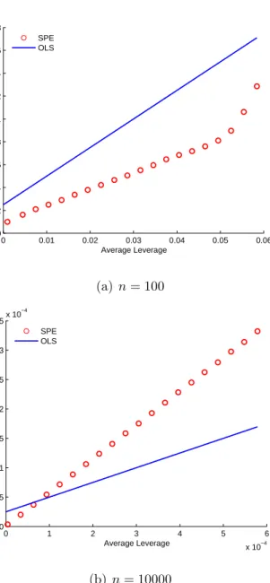
The numerical study begins withk = 3, β0 = 1, β =1, N = 100,000, np = 21, σ2

ξ = 0.25, andξp =0. We run two experiments: one has a calibration set with a

size of 100, and the other has 10000 observations in the calibration set. We set up the number of bins in the uniform binning method to be 20. An average squared prediction error against average leverage plot is used to show the relationship as shown in Equation (2.4), that describes the dependence of prediction error on xp

(via h). To avoid noise, we use the true value of σ2

ξ in the ordinary least squares

(35)

relationship that should be reproduced by the simulation can be written as Var ( ˙yp−yˆ˙p) =σξ2(

1

n +h). (2.7)

In Figure 2.2, the blue line shows the linear relationship described in Equation (2.7), and the red points display the actual relationship between the squared pre-diction error and the leverage observed in the simulation. In Figure 2.2(a), the blue line has an intercept of σ

2

ξ

n = 0.0025, and the slope of σ

2

ξ = 0.25. In Figure

2.2(b), the intercept of the blue line is equal to σ

2

ξ

n = 0.000025, and its slope is still

equal toσ2

ξ = 0.25.

As the squared prediction error ˆξ2

pj is proportional to rj, and the leverage hj ≈

rj

n, the red points are supposed to form a straight line. But in Figure 2.2(a)

the last four red points are bent up. The curvature appears because _n1Ik does not

give a good approximation of (X′

cXc)−1 whenn= 100, which causes the curvature

at the tail. In other words, if the sample size is large, the approximation would work well. The leverage has a better uniform distribution. It is why in Figure 2.2(a) the red points are perfectly linear when n = 10000.

As for a prediction sample xpj, the uniformly distributed leverage design

en-forces both squared prediction error and leverage to be proportional torj. In fact,

for a fixed calibration set, the true relationship between squared prediction error and leverage may not be linear, which has been discussed in Simulation 2.1 where Figure 2.1(a) is a typical example. Hence, the uniformly distributed leverage de-sign distorts the true relationship between squared prediction error and leverage for a fixed calibration set. Moreover, for principal components regression and partial least squares regression, the distribution of the predictors will affect the relationship between the bias and the leverage, so the simulations with uniformly distributed leverage would fix the pattern of this relationship in an unnatural way. Hence, the predictors with a multivariate normal distribution would be more appropriate.

Simulation 2.3. Three Different Simulations ofyc for a Fixed Xc

(36)

Chapter 2. OLS Prediction Uncertainty 0 0.01 0.02 0.03 0.04 0.05 0.06 0 0.002 0.004 0.006 0.008 0.01 0.012 0.014 0.016 0.018

Average Leverage SPE OLS (a) n= 100 0 1 2 3 4 5 6 x 10−4 0 0.5 1 1.5 2 2.5 3 3.5x 10 −4

OLS

(b) n= 10000

Figure 2.2: OLS Average Squared Prediction Error versus Average Leverage, uni-formly distributed leverage, Case (1) a fixed calibration set ( ˙Xc,y˙c). SPE: average

squared prediction error ( ˙yp −yˆ˙p)2 against average leverage h = xp(X′cXc)−1x′p.

OLS: the ordinary least squares prediction variance, Var ( ˙yp−yˆ˙p) = σ2ξ(

1

n+h) (See

(37)

100,000 replicates. Each experiment has a set of explanatory variables, but dif-ferent replicates of the response variable are simulated for the fixed calibration set. The parameters are set as the same as Simulation 2.1. There are three plots displayed in Figure 2.3, they compare the relationship of observed squared pre-diction error against leverage and theoretical prepre-diction variance against leverage. The red points present average squared prediction error against average leverage for the particular set of the response variable. The blue line presents the ordinary least squares prediction variance given by Equation (2.7).

In Figure 2.3(a), the slope of the red line is similar to the blue line; in Figure 2.3(b) the slope of the red line is smaller than that of the blue line; in Figure 2.3(c) the slope of the red line is bigger than that of the blue line. The red lines can be steeper, flatter, or similar to the blue lines. This is because red points in the three graphs are drawn for three different simulations of the response variable in the calibration sets. And, the curvature formed by the red points is decided by the distribution of explanatory variables in the calibration set, which has been explained in Simulation 2.1.

The blue line in Figure 2.3 is an expected value over repeated sampling of yc, and does not describe the behavior of the errors for fixed yc. The

perfor-mance of the ordinary least squares regression prediction variance formula cannot be assessed in the obvious way referring to a fixed dataset, because the prediction variance formula takes expectation over the distribution of the estimated regres-sion coefficients, and the squared prediction error calculated for a single set of data always relies on the estimated regression coefficients from this dataset. It is im-portant to be aware of this behavior of the prediction variance formula in order to study prediction uncertainty of principal components regression and partial least squares regression.

Additional problems that will arise with real data sets are the availability of prediction samples, and the presence of noise in the predictions. Each red point in the plot of Figure 2.3 is an average over 100,000 squared prediction errors against their leverages, and the regression variance in the prediction set σ2

(38)

Chapter 2. OLS Prediction Uncertainty 0 0.02 0.04 0.06 0.08 0.1 0.12 0 0.005 0.01 0.015 0.02 0.025 0.03

OLS

(a) First simulation of ˙yc for a fixed ˙Xc

0 0.02 0.04 0.06 0.08 0.1 0.12 0 0.005 0.01 0.015 0.02 0.025 0.03

OLS

(b) Second simulation of ˙yc for a fixed ˙Xc

Figure 2.3: OLS Average Squared Prediction Error versus Average Leverage, uni-formly distributed leverage, three simulations of yc for a fixed Xc. SPE: average

squared prediction error ( ˙yp −yˆ˙p)2 against average leverage h = xp(X′cXc)−1x′p.

(39)

0 0.02 0.04 0.06 0.08 0.1 0.12 0 0.005 0.01 0.015 0.02 0.025 0.03 0.035 0.04 0.045

OLS

(c) Third simulation of ˙yc for a fixed ˙Xc

Figure 2.3: OLS Average Squared Prediction Error versus Average Leverage, uni-formly distributed leverage, three simulations of yc for a fixed Xc (cont.).

zero. For a real dataset, it is difficult to collect the data with such a large number of predictions, and the noise term always exists. Hence, the red points are unlikely to form such a clear straight line.

With real data sets, we need to find some way to round the assessment difficulty. We will try to model the linear relationship shown in the ordinary least squares prediction variance formula empirically, via the use of the tuning set (Section 2.2.3) or cross-validation (Section 2.2.4). And then, we will investigate whether random data splitting (Section 2.2.5) can be used to round the assessment difficulty or not.

2.2.3 The Use of a Tuning Set

In Section 1.1 we have shown that a tuning set ( ˙Xt,y˙t) sampled from the same

distribution as the calibration set can be useful in the quantification of prediction uncertainty in the ordinary least squares regression, where the number of observa-tions in the tuning set is denoted as nt. After we obtain the estimated regression

coefficients from the calibration set, the tuning set can be used in two different ways. One is to calculate the root mean squared error of prediction (Equation (1.8)) as an empirical estimate of prediction error. The other way is to use the

(40)

Chapter 2. OLS Prediction Uncertainty estimate of regression error variance (Equation (1.9)) from the tuning set in the ordinary least squares prediction variance formula. The tuning set can also be used as the same way in the study of principal components regression and partial least squares regression. In this section, we would like to study whether a tun-ing set can be used to provide a sensible empirical estimate of the ordinary least squares prediction variance formula, so that it can provide an approximation to the prediction variance for a real dataset. We hope this would shed some light on using the tuning set in principal components regression and partial least squares regression.

For a real dataset, the calibration set is fixed. Although in this case the re-lationship between squared prediction error and leverage may not be linear as shown in Equation (2.6) Simulation 2.1, the ordinary least squares prediction vari-ance formula can be used as an approximation to prediction varivari-ance. Since the ordinary least squares prediction variance formula gives a linear relationship be-tween squared prediction error and leverage, would it be possible to quantify the approximate predication variance through estimating the slope and the intercept of the formula? If possible, how many samples are needed in the tuning set in order to give reasonable estimates of the slope and the intercept? Is there any relationship between the sample sizes n and nt? To answer these questions, we

consider the relationship between the squared prediction error ˆξ2_t and the leverage ht calculated in the tuning set.

For a calibration set ( ˙Xc,y˙c) and a tuning set, ˙Xc ∼ N(0,Σ) and ˙Xt ∼ N(0,Σ), where Σ is the covariance matrix. Assume Σ=CC′_{, thus (X}′

cXc)−1 ≈

1

n(CC

′₎−1_{. For a sample in the tuning set, the transformation of the centred} predictorC−1_x′

t∼N(0,Σ), which givesxt(CC′)−1x′thas a Chi-square distribution

with k degrees of freedom.

xt(C′)−1C−1x′t=xt(CC′)−1x′t∼χ2k.

The leverageht =xt(X′cXc)−1x′t ≈xt_n1(CC′)−1x′t, which has approximately a

Chi-square distribution _n1χ2

k. E (ht) = k_n and Var (ht) = 2_nk. E{Pn_i₌₁t (hti−¯ht)

2_{} ≈} 2knt

(41)

The ordinary least squares prediction variance formula gives a linear relation-ship between leverage and prediction variance. We could use this relationrelation-ship to build a linear model to regress squared prediction error on leverage for the tun-ing set, thus givtun-ing empirical estimates how prediction variance associates with leverage. Assume the simple linear model as

ˆ

ξ2_t =ω0+ω1ht+ν, (2.8)

where ˆξ2_t denotes the squared prediction errors, ht denotes the leverages in the

tuning set, and ν is the noise term. The regression coefficient ω0 is the intercept, and ω1 is the slope. According to the ordinary least squares regression theory,

σ2

ν = Var (ξt2) = 2σξ4. ˆω1 ≈σξ2, so the variance of the estimated slope

Var (ˆω1) = σ 2 ν Pnt i=1(hti−¯ht) 2 ≈ 2σ4 ξ 2knt/n = σ 4 ξn knt .

The coefficient of variation of ˆω1

c.v.(ˆω1) = p Var (ˆω1) ˆ ω1 = s σ4 ξn knt /σ2 ξ = r n knt . (2.9)

Intuitively, for fixed n and nt, when there are more predictors, the leverage

in-creases on average. If we study squared prediction error at a certain level, when larger leverages account more for the deterministic part of the linear model (See Equation (2.8)), the estimated regression coefficient ˆω1 is more stable. Usually ˆ

ω1 is good enough as an estimate of the slope when c.v.(ˆω1) is less than or equal to 0.1000 in magnitude. We often use ordinary least squares regression when the number of explanatory variables less than or equal to 7. Whenk = 7, n = 10 and

nt = 100, Equation (2.9) gives c.v.(ˆω1) = 0.1195, which suggests the size of the

tuning set should be at least 10 times of the size of the calibration set. In the real situation, it is difficult to obtain such a large size tuning set. When the calibration set and tuning set have equal size, c.v.(ˆω1) ≤ 0.1000 requires k ≥ 100. This is unrealistic because when there are more than 10 explanatory variables we usually do not employ ordinary least squares regression.

In Simulation 2.1 Case (1) when k = 3, suppose there is a tuning set that has equal size with the calibration set nt = n = 100, c.v.(ˆω1) =

q

1

3 ≈ 0.5774. When

(42)

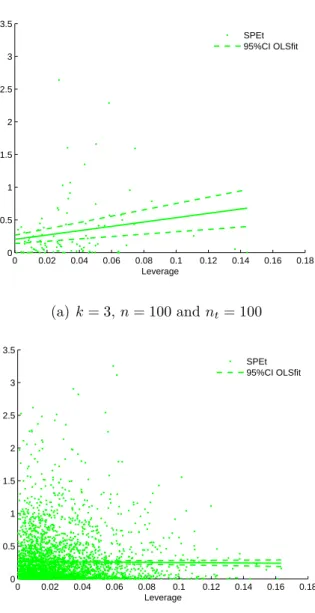
Chapter 2. OLS Prediction Uncertainty 0 0.02 0.04 0.06 0.08 0.1 0.12 0.14 0.16 0.18 0 0.5 1 1.5 2 2.5 3 3.5

Squared Prediction Error

Leverage SPEt 95%CI OLSfit (a) k= 3,n= 100 andnt= 100 0 0.02 0.04 0.06 0.08 0.1 0.12 0.14 0.16 0.18 0 0.5 1 1.5 2 2.5 3 3.5

Squared Prediction Error

Leverage

SPEt 95%CI OLSfit

(b) k= 3,n= 100 andnt= 3333

Figure 2.4: OLS Squared Prediction Error versus Leverage in a Tuning Set, i.i.d. standard normally distributed predictors, one ( ˙Xc,y˙c). SPEt: squared prediction

error in the tuning set ( ˙yt −yˆ˙t)2 against leverage ht = xt(X′cXc)−1x′t. 95%CI

OLSfit: 95% confidence interval of the ordinary least squares fit of all squared prediction errors against leverages in the tuning set.

(43)

Figure 2.4 displays the result of an experiment of Simulation 2.1 Case (1),

k = 3, n = 100, where the green point denotes squared prediction error against leverage in a tuning set. The two green dash lines give the 95% confidence interval of the ordinary least squares fit of all squared prediction error against leverage in the tuning set. The solid green line is drawn by ˆξ2_t = ˆω0 + ˆω1ht. Figure 2.4(a)

plots the case whennt = 100 and (b) presents the case whennt= 3333. The 95%

confidence interval band in (a) is much wider than that in (b) given the two plots are drawn on the same scales. This suggests that when nt = 100 the estimated

slope is more variable than that when nt = 3333, which is consistent with the

coefficient variations where (a)c.v.(ˆω1)_≈0.5774 and (b) c.v.(ˆω1)_≈0.1000. In theory, the ordinary least squares prediction variance formula can be esti-mated empirically by conducting a simple linear regression of squared prediction error against leverage in a tuning set. However, the realisation of this method requires a minimum size of the tuning set according to the number of explanatory variables and the sample size of the calibration set. In practice, the number of explanatory variables, the sample sizes of the calibration and the tuning sets can-not coordinate easily to generate reliable regression coefficient estimates for the ordinary least squares prediction variance formula. Hence, it would be difficult to calculate the approximate prediction variance for a real dataset in this way. It is unnecessary to study the tuning set like this in principle components regression and partial least squares regression.

2.2.4 Cross-validation

Before studying principal components regression and partial least squares regres-sion, we study validation in ordinary least squares regression. The cross-validation can be used in the same way as the tuning set. From the cross-cross-validation, we are able to calculate an empirical estimate of prediction error and an estimated regression error variance, which also applies in principal components regression and partial least squares regression. We present how to carry out the cross-validation as below.

(44)

Chapter 2. OLS Prediction Uncertainty Definition 2.3. Cross-validation

Leave-one-out cross-validation builds reduced data sets by deleting one obser-vation each time. ( ˙Xc₋j,y˙c−j) is the new dataset constructed by leaving out the j-th observation ( ˙xcj,y˙cj), that is,

˙

Xc−j = ( ˙xc1, . . . ,x˙cj−1,x˙cj+1, . . . ,x˙cn)

˙

yc−j = ( ˙yc1, . . . ,y˙cj−1,y˙cj+1, . . . ,y˙cn)

′ _j _{= 1}_{, . . . , n}

After the new dataset is generated, the leave-out observation is used as the pre-diction.

When it comes to estimating empirically the approximate prediction variance presented by the ordinary least squares prediction variance formula for a real dataset, cross-validation can be taken as the case when using a tuning set with

nt = n, so the coefficient variation c.v.(ˆω1) =

q

1

k (See Equation (2.9)). If we

set c.v.(ˆω1) ≤ 0.1000, the number of explanatory variables needs to be at least 100. A large number of explanatory variables ensures ˆω1 to be estimated properly as c.v.(ˆω1) is very small in this case. However, it does not make sense to apply ordinary least squares regression for such a large number of explanatory variables. Likewise, we will not use cross-validation in this way for principal components regression and partial least squares regression.

2.2.5 Random Data Splitting

In this section, we will investigate whether random data splitting can be a useful tool or not, to round the problem that the performance of the ordinary least squares prediction variance formula cannot be assessed by any single data sets directly. If we want to use random data splitting in the study of principal components regression and partial least squares regression, it should work in ordinary least squares regression.

Simulation 2.4. Random Data Splitting for One Set of Simulated Data

(45)

randomly permuted and split into a calibration set with n observations, a tuning set with nt observations, and a prediction set with np observations. The three

data sets are exchangeable. Estimated regression coefficients are calculated from the calibration set, and are used to make predictions for the tuning set and the prediction set. Squared prediction errors and leverages in both of the tuning set and the prediction set are saved to be compared.

In order to investigate how the noise of the dataset make an influence on the result, we fix the noise term in the prediction set to beξ_p = 0.25. The regression model can be written as

˙ yc = β0+ ˙Xcβ+ξc, ˙ yt = β0+ ˙Xtβ+ξt, ˙ yp = β0+ ˙Xpβ+ξp.

The parameters of the numerical experiment are configured as following. N = 100000, k = 1, ˙Xc ∼ N(0,1), β0= β1=1, σξ2 = 0.25, n = 200, nt = 200, and np = 200.

In Figure 2.5, the green point (SPEt) stands for average squared prediction error against average leverage calculated from the tuning set. The green line (SPEt fit) is the ordinary least squares fit of all squared prediction error against leverage in the tuning set. The pink point (SPE) presents average squared prediction error against average leverage. The pink dash line (SPE fit) is the ordinary least squares fit of all squared prediction error against leverage. The light blue line (OLS) is given by the ordinary least squares regression variance where σ2

ξ = 0.25

for simplicity.

The pink points form a straight line (SPE fit). The light blue line (OLS) and the pink dash line (SPE fit) overlap, because the error term is fixed as 0.25. The green points (SPEt) are so noisy that the green line (SPEt OLSfit) is quite different from the blue and pink lines.

If the error term in the prediction set is not fixed, the tuning set and the prediction set would have exactly the same result because the tuning set and the prediction set are exchangeable. The noisy green points Figure 2.5 suggests it is