Article
Canopy Reflectance Modeling of Aquatic
Vegetation for Algorithm Development:
Global Sensitivity Analysis
Guanhua Zhou1,2,3,*ID, Zhongqi Ma1, Shubha Sathyendranath2,4, Trevor Platt2,4, Cheng Jiang5,6and Kang Sun3
1 School of Instrumentation Science and Opto-electronics Engineering, Beihang Univerisity, Beijing 100191, China; [email protected]
2 Plymouth Marine Laboratory, Prospect Place, Plymouth PL1 3DH, UK; [email protected] (S.S.); [email protected] (T.P.)
3 CETC Key Laboratory of Aerospace Information Applications, Shijiazhuang 050081, China; [email protected]
4 National Centre for Earth Observation, Plymouth Marine Laboratory, Prospect Place, Plymouth PL1 3DH, UK
5 Beijing Institute of Space Mechanics & Electricity, Beijing 100094, China; [email protected] 6 Key Laboratory for Advanced Optical Remote Sensing Technology of Beijing, Beijing 100094, China * Correspondence: [email protected]; Tel.: +86-010-82315884
Received: 28 April 2018; Accepted: 24 May 2018; Published: 27 May 2018
Abstract: Optical remote sensing of aquatic vegetation in shallow water is an essential aid to ecosystem protection, but it is difficult because the spectral characteristics of the vegetation are sensitive to external features such as water background effects, atmospheric effects, and the structural properties of the canopy. A global sensitivity analysis of an aquatic vegetation radiative transfer model provides invaluable background for algorithm development for use in optical remote sensing. Here, we use the extended Fourier Amplitude Sensitivity Test (EFAST) method for the modelling. Four different cases were identified by subdividing the ranges of water depth and leaf area index (LAI) involved. The results indicate that the reflectance of emergent vegetation is affected mainly by the concentrations of chlorophyll a + b in leaves (Cab), leaf inclination distribution function parameter (LIDFa) and LAI. The parameter LAI is influential in sparse vegetation cases whereas Cab and LIDFa are influential in dense vegetation cases. Canopy reflectance for submerged vegetation is dominated by water parameters. Relatively, LAI and Cab are highly sensitive vegetation parameters. The analysis is extended to vegetation index as well, which takes the Sentinel-2A as the reference sensor. It shows that NDAVI (Normalized Difference Aquatic Vegetation Index) is suitable for retrieving LAI in all cases except deep-sparse for emergent vegetation, whereas NDVI (Normalized Difference Vegetation Index) would be better in the deep-sparse case. NDVI, NDAVI and WAVI (Water Adjusted Vegetation Index), respectively, are suitable for retrieving Cab, Car and LIDFa in dense cases. For submerged vegetation, the sensitivity of LAI to NDAVI is relatively high only in the shallow-sparse case. The adjustment factorLin SAVI and WAVI fails to suppress the sensitivity to water constituent parameters. The sensitivity of LAI and Cab to NDVI in deep cases is relatively higher than that to the other indices, which may provide clues for the construction of inversion algorithms in macrophyte remote sensing in the aquatic environment using spectral signatures in the visible and near infrared regions.
Keywords:aquatic vegetation; radiative transfer model; global sensitivity analysis; vegetation index; Sentinel-2A; wetland remote sensing
1. Introduction
Aquatic vegetation is a key element in the sustainability of wetland ecosystems [1,2]. According to growth habitat, aquatic vegetation can be divided into three groups: emergent vegetation, whose roots grow in the sediment underwater but whose leaves and stems emerge out of water; floating vegetation, which has leaves floating just above the water surface; and submerged vegetation, which lives entirely below the water surface [3]. These plants serve to absorb nitrogen and phosphorus, reduce turbidity and inhibit eutrophication, and can be used as indicators of the trophic status of a water body. It is important to monitor the distribution of aquatic vegetation as an aid to protecting wetland ecosystems. Conventional field surveys of macrophyte communities are difficult to implement, requiring considerable time and expense to carry out over large spatial scales [4]. Even worse, traditional field-based surveys are commonly hindered by limited accessibility [5]. The technology of remote sensing has the advantage of a broad coverage and frequent data acquisitions, which makes it a valuable tool for the assessment of macrophyte distribution, vegetation status and related biophysical parameters.
At present, the technologies of remote sensing are widely used for mapping and classification of aquatic vegetation [6–8]. Another major application of wetland remote sensing is parameter inversion, which includes mainly biomass [9–12] and leaf area index (LAI) [13,14]. The inversion is usually based upon statistical methods that contain no fundamental mechanistic information about the optical properties of the vegetation itself. Moreover, the data required by the statistical methods are specific to the particular species in a particular region, which limits their accuracy when applied to other species or regions. It is mainly because of the complex growth environment, which has a significant impact on the spectral properties of the vegetation, that many scholars prefer statistical methods to mechanistically-based methods. As for emergent vegetation and floating vegetation, their spectra are similar to those of terrestrial vegetation with a green reflectance peak and “red edge”, but the canopy reflectance will decrease with vegetation density as there will be more water exposed in the background causing attenuation, especially in the near-infrared (NIR) region [15]. Submerged vegetation is characteristic of deeper water. The strong absorption of water forces the canopy reflectance to be attenuated by a factor of order 100 [16]. In addition to water itself, optically active materials in the water (i.e., phytoplankton, pigments and yellow substances) can also affect the observed signal [17]. Thus, to improve the accuracy of inversion, it is imperative to understand the relative importance of interactions among the factors that influence reflectance in the macrophyte-water coupled system.
To achieve this goal, a radiative transfer model for aquatic vegetation is required. Exploration of the radiative transfer process and analyses of the reflectance spectra of aquatic vegetation have increased in recent years. Currently, there are several models available that are able to simulate the spectral response of aquatic vegetation [18–25]. We have proposed the Aquatic Vegetation Radiative Transfer model (AVRT) based on the SAIL model framework. The model stratifies the whole system and calculates the scattering matrix for each layer separately [26]. The bidirectional reflectance of the whole system is calculated after iterative accumulation. The AVRT model can calculate the spectra of emergent vegetation, submerged vegetation and floating vegetation in the band range of 400–1000 nm. This model is validated with in-situ spectral data and with a more accurate Monte Carlo model. By a holistic analysis of the sensitivity of reflectance, based on model simulation, we have been able to obtain a better understanding of the interactions between environmental factors and aquatic vegetation. Global sensitivity analysis is an excellent method to quantify the relative importance of each input variable to model output, and therefore to identify the key determinants of output such as reflectance. It can also help set reasonable default values under a relatively wide range of conditions for less influential variables [27]. Then we can try to retrieve the key parameters of wetlands from field spectra or images, and develop new approaches to extract more optical information about various wetland species. This work can facilitate the dynamic monitoring of wetlands and, finally, can benefit the protection of wetland ecosystems.
The law of parsimony says that only a few input variables can account for most of the effects on the output response, so identifying these important parameters is essential for complex models with many input variables. Sensitivity analysis can be an effective tool to discriminate the effects of the models’ various parameters [28]. Sensitivity analysis refers to calculation of how the uncertainties in a model’s output should be assigned, qualitatively or quantitatively, to uncertainties in the various inputs. Generally, it can be classified into local sensitivity analysis and global sensitivity analysis. Local sensitivity analysis methods are often referred to as “one-factor-at-a-time” (OAT), because they change the value of one variable at a time while holding all others at their central values, then measuring variation in the outputs. Local sensitivity analysis can analyze the impact of only a single input parameter on the outputs and does not encompass the entire input variable space [29]. Thus, local sensitivity analysis methods are inadequate for analyzing complex models, with many variables, that may be highly dimensional as well as non-linear. However, global sensitivity analysis explores the full input variable space and can elucidate not only the main effect of each parameter but also the secondary or higher order interactions among parameters [28]. The commonly used global sensitivity analysis methods include correlation-based methods [30], variance decomposition methods [31] and density-based methods [32]. Sensitivity analysis has been widely used in various regimes [28]. Recently, some scholars have used global sensitivity analysis to discuss the properties of the models implemented in remote sensing [33,34]. Several papers in which sensitivity analysis is used for research on terrestrial vegetation also deserve attention. Xiao et al. analyzed the well-known canopy model Prosail by the extended Fourier Amplitude Sensitivity Test (EFAST) method. The analysis showed that LAI had the most significant effect on canopy reflectance for sparse canopy with LAI in the range of 0–3. For dense canopies (LAI = 3–6), the concentrations of Chlorophyll a and b in leaves were the most influential parameters in the visible region [35]. Mousivand et al. obtained the sensitivity not only of the canopy reflectance but also the Top-Of-Atmosphere (TOA) radiance of a soil-vegetation system, and the analyzed factors, including the biophysical and biochemical parameters of a coupled Soil–Leaf-Canopy model and Modtran. They found that crown coverage, LAI, leaf inclination distribution function (LIDF) and soil moisture were the most influential parameters in the range 400–2500 nm [36]. Verelst et al. used machine-learning methods to simplify several radiative transfer models (i.e., Prospect-4, Prosail, and Modtran-5). The simplified versions had the same sensitivity patterns as the original ones. Among them, the results of Modtran-5 showed that aerosol optical parameters such as AOT and Angstrom Coefficient had very significant effects in the range 400–2500 nm [37]. Aquatic vegetation indices and their related sensitivity analysis in reflectance spectra have recently been reported [38]. However, the model used in this work for aquatic vegetation is a terrestrial vegetation model applied in an aquatic context. The impacts of some parameters such as water depth and concentrations of water constituents, which should be of distinct importance especially for submerged vegetation, are not discussed. A systematic sensitivity analysis of the reflectance spectra of various types of aquatic vegetation should be helpful for developing practical aquatic vegetation indices and for retrieving biophysical or biochemical parameters.
The goal of this work is to determine which parameters of the coupled macrophyte-water system can be retrieved from remote sensing measurements and under what conditions. This would help in developing or refining inversion algorithms for aquatic vegetation or optically-complex waters. In addition, by identifying variables of only minor influence, models can be greatly simplified, which facilitates inversion applications [39]. The EFAST method proposed by Saltelli et al. [27] will be utilized to analyze the global sensitivity of vegetation, water parameters and boundary conditions, as this method achieves both accuracy and efficiency. The AVRT model will be utilized to simulate a large data set, which takes the variation of different parameters into consideration, and is analyzed via EFAST. It should be emphasised that the sensitivity analysis in this study is performed on the simulation data (no field measured data used), since most of parameters considered are not controllable in field measurement, which brings difficulties to the sensitivity analysis. In this paper, the global sensitivity analysis includes the following two parts: (1) to analyze
the sensitivity of AVRT model input parameters to canopy spectra in several cases which are set by subdividing the range of water depth and LAI; and (2) to analyze the sensitivity of input parameters to conventional terrestrial vegetation indices NDVI, SAVI, and aquatic vegetation indices NDAVI and SAVI in several cases, because these broadband vegetation indices are widely used and perform well in applications of multispectral satellite data, which is an important data source in wetland remote sensing. Unlike the use of ocean-color satellite data in deep waters for studying phytoplankton concentration, which relies on spectral signatures in the visible domain, detection of vegetation in shallow-waters requires that we use spectral signatures in both visible and near infrared domains. The spectral response functions of Sentinel-2A can be used to calculate the band equivalent reflectance and then to obtain the vegetation index mentioned above. Because the optical response of floating vegetation is very similar to that of emergent vegetation, and because emergent vegetation is more representative, the targets in this paper are emergent vegetation and submerged vegetation.
The rest of the paper is organized as follows: in Section2the AVRT model and the EFAST method used in the paper are briefly introduced. Section3shows the ranges and distributions of model input parameters and introduces the spectral advantages of Sentinel-2A for monitoring aquatic vegetation in shallow water bodies, and explains the motivation for selecting Sentinel-2A as the reference sensor. In Section4, the results of the two parts mentioned above are presented. Section5 states the comprehensively discussion about these results. Finally, Section6concludes this paper and suggests directions for future research.
2. Methodology 2.1. AVRT Model
To discuss adequately the interactions between water columns and vegetation while maintaining a balance between accuracy and efficiency, we adopt some basic assumptions in the AVRT model: (1) the whole system can be divided into several layers, in vertical direction, whose optical properties are homogeneous. A single layer can be water, vegetation or the water-vegetation mixed medium; (2) the thickness of the water surface is taken as zero; (3) the bottom is assumed to be Lambertian.
The type of medium in each layer is determined mainly by the water depth, plant height, LAI and the volume fraction of water. If the water depth is greater than the plant height, submerged vegetation is taken as the object and each layer in the system is considered, partly or totally, to contain water, which means it could be water or the mixed medium. Otherwise, the system could be emergent vegetation or floating vegetation, and each layer could be vegetation or the mixed medium. Furthermore, if LAI of a certain layer is larger than the threshold, it is determined that this layer must contain vegetation. And if this layer has been judged to contain partly water, it is determined to be the mixed medium. It is logically similar for the volume fraction of water when deciding whether the layer is water or mixed medium.
The entire system also includes the air-water interface and the bottom. After deciding each layer type, the scattering matrix, which includes the reflectance and transmittance, is calculated according to the optical properties of the medium. In the AVRT model, PROSEPCT-5 [40] is utilized to calculate the reflectance and transmittance of a single leaf, and after that it is used in the modified SAILH model to calculate the scattering coefficients of vegetation. The scattering and absorption characteristics of the water column are determined by bio-optical models [41–46]. The Cox-Munk [47] model is utilized to calculate the surface scattering matrix. The detailed calculation process is presented in Zhou et al. [26]. The reflectance matrix of the whole system is calculated using an iterative adding method, which refers to Cooper et al. [48] and Verhoef [49]. Considering both direct and diffuse incident radiations, the canopy bidirectional reflectance can be obtained.
In this paper, the AVRT model is utilized to simulate the canopy spectra of emergent vegetation and submerged vegetation. Apart from the bottom and water surface, the whole system is divided for simplicity into two layers. The lower layer is the water-vegetation mixed medium for both emergent
vegetation and submerged vegetation. The upper layer for emergent vegetation is the vegetation medium, and that for submerged vegetation is the water medium. The input parameters required in the simulation will be introduced in Section3.1.
2.2. EFAST Method
This section will introduce the EFAST method. It is the extended version of FAST method. When analyzing the model defined asy = f(x1,x2, . . . ,xn)in the FAST method, a curve is defined as Equation (1) to explore then-dimensional space of input parameters [27]:
xi(s) = Gi(sinωis),∀i = 1, 2, . . . ,n, (1) wherexistands for thei-th input parameter,sis an independent variable,Gi is the transformation function and ωi is a frequency associated with each input parameter. Ass varies, all the input parameters change along the curve simultaneously inn-dimensional space. Every input oscillates periodically at its corresponding frequency ωi. If xi has significant impact on the model output y, it should have high amplitude at its frequency ωi. After Fourier expansion, the model
f(x1(s),x2(s), . . . ,xn(s)) = f(s)can be expressed as Equation (2):
f(s) = +∞
∑
j=−∞ Ajcosjs+Bjsinjs ,j∈Z, (2)where Aj andBj are the Fourier coefficients. The spectrum of the Fourier expansion was defined asΛj = Aj2+Bj2. Because f(s)was a real-valued function, they are symmetrical and could be expressed as:A−j = Aj,B−j = −Bj,Λ−j = Λj. Therefore, the output varianceDiarising fromxi and the total varianceDcould be estimated by adding the spectra:
Di =
∑
p∈Z0 Λpωi = 2 +∞∑
p=1 Λpωi, (3) D =∑
j∈Z0 Λj = 2 +∞∑
j=1 Λj, (4)whereZ0means all integers except the 0. The first order sensitivity indexSiofxicould be: Si =
Di
D. (5)
After that, Saltelli et al. [27] combined the idea of the variance decomposition method with that of the FAST method. The total output variance would be decomposed into the variance associated with each input or the interactions among the input parameters.
To determine the total sensitivity indexSTi ofxi, the frequency of xi was set toωi while the frequency of the rest of input parameters wasω−i, which is different from . The symbol−irefers to the complementary set ofi. After calculating the spectrum at the frequencyω−iand higher harmonics pω−i, the partial varianceD(−i)could be obtained just as in Equation (4). It means that the variance unrelated toxi, then the varianceDTiwhich is the complementary set ofD(−i)could be calculated by subtractingD(−i)fromD.STicould be defined as:
STi = D−D(−i)
D . (6)
The total sensitivity indexSTidescribes the impact ofxiand the interactions betweenxiand the rest of input parameters on the model output. It is more comprehensive than the first order sensitivity
index. Obviously, the sum of first order sensitivity indices of all input parameters should be less than 1 whereas the sum of total order sensitivity indices will be greater than 1. This sum would equal 1 only if all the interaction items were zero.
The calculation process of EFAST is introduced in detail in AppendixA. In this paper, we will follow the process to make the global sensitivity analysis. The ranges and distributions of all the input parameters of AVRT will be introduced in Section3.1.
3. Data
In this section, the variability ranges and distributions of the input parameters are introduced. They are significant to sampling. After sampling, the input data set is entered into the AVRT model to simulate the canopy spectra of emergent vegetation and submerged vegetation in the range of 400–1000 nm, the global sensitivity analysis (abbreviated as GSA) is performed for each wavelength to obtain the high sensitivity band ranges of each parameter. Next a description of Sentinel-2A satellite is given, including the band settings and the spectral response functions, which are used to calculate first the band equivalent reflectance and then the vegetation index.
3.1. Input Parameters
A systematic exploration of the parameter space is necessary for GSA. It is important to select an approximate and representative sample set, because the macrophyte-water coupled system is too complicated to test all possible combinations of parameter values. Efficient sampling of the parameter space requires some priori knowledge of the probability distribution of parameter values. This ensures that unlikely or implausible parameter values and unlikely combinations are not given equal weight to the more likely ones [36]. The input parameters of AVRT could be divided into vegetation parameters, water column parameters and the boundary conditions. The ranges and descriptions of the input parameters are given in Table 1. The ranges of leaf biophysical parameters refer to the technical documents of PROSEPCT-5. The ranges of water column parameters refer to the field measurements reported in relevant papers (such as Cchla [43] and SPM [50]), and the ranges set by the bio-optical models (Btsm [46] and aCDOM [51]).
Due to the lack of priori knowledge, the probability distributions of all parameters are set to uniform, that is all parameters are equally likely to be found anywhere in their range of variation. The results of the GSA could change when the range of variation of the parameters changed. Therefore, it is of great importance to establish several cases by combining different parameter ranges, which could also reveal the sensitive conditions for each parameter. In this paper, the water depth is divided into shallow (0.1–1.0, unit: m) and deep (1.0–2.0, unit: m) conditions, which reflect the strength of the attenuation caused by water columns. The range of LAI is set to sparse (0–2, dimensionless) and dense (2–4, dimensionless) to represent the extent of vegetation cover. After a couple of combinations, four cases can be obtained: shallow-sparse, shallow-dense, deep-sparse and deep-dense. The observation conditions are shown at the end of Table1.
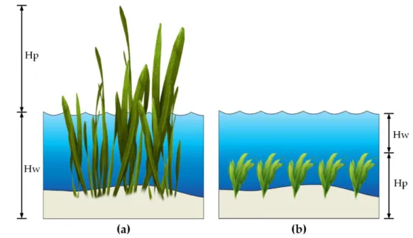
As mentioned in Section2.1, the system is divided into two layers for emergent vegetation and submerged vegetation. So, the definitions of Hw and Hp in Table1are actually the height of a single layer in the system. A detailed schematic of vertical structures for the two kinds of vegetation is shown as Figure1. In Figure1a, Hw is the height from bottom to the water surface, that is, the actual water depth, which represents the height of the water-vegetation mixed medium. Hp is the height from the water surface to the top of the canopy, which represents the height of the layer totally full of vegetation. As for submerged vegetation, Hp is the height from bottom to the top of the canopy, that is, the actual plant height, which represents the height of the mixed medium. Hw is the height from the top of the canopy to the water surface, which represents the height of the water layer.
Table 1.The descriptions and ranges of input parameters. The observation conditions are indicated at the end of Table1, which include solar and viewing zenith angle and the relative azimuth angle in air.
Parameter Description Unit Range
Hw1 Water depth for emergent vegetation
The height of the upper water layer for submerged vegetation m
0.1–1.0 (Shallow) 1.0–2.0 (Deep) Hp The height of the upper vegetation layer for emergent vegetationPlant height for submerged vegetation m 0.1–1.0
N Leaf structure parameter — 1–2.5
Cab Concentration of chlorophyll a + b, in leaves µg/cm2 10–80 Car Concentration of carotenoid, in leaves µg/cm2 10–30 Cw Concentration of equivalent water thickness, in leaves µg/cm2 0.004–0.04 Cm Concentration of dry matter, in leaves µg/cm2 0.002–0.01
LAI Leaf area index — 0–2 (Sparse)
2–4 (Dense) LIDFa Leaf inclination distribution function parameter a
(which represents the average leaf slope) — −1–1 LIDFb Leaf inclination distribution function parameter b
(which represents the distribution’s bimodality) — −1–1 Fw volume fraction of water in a layer — 0.7–1 Cchla Concentration of chlorophyll a, in water mg/m3 0–80 Btsm Coefficient to calculate scattering of total suspended matter — 1–5 SPM Concentration of suspended matter, in water g/m3 0–80 aCDOM Absorption coefficient of CDOM at 375 nm /m 0.5–3
Rbtm Reflectance of bottom — 0–1
SZA Sun zenith angle in air degree 30
VZA Viewing zenith angle in air degree 0 RA Relative azimuth angle in air degree 0
1For both of emergent vegetation and submerged vegetation, the ranges of Hw are the same.
Remote Sens. 2018, 10, x FOR PEER REVIEW 7 of 22
2–4 (Dense) LIDFa Leaf inclination distribution function parameter a
(which represents the average leaf slope) — −1–1 LIDFb Leaf inclination distribution function parameter b
(which represents the distribution’s bimodality) — −1–1 Fw volume fraction of water in a layer — 0.7–1 Cchla Concentration of chlorophyll a, in water mg/m30–80
Btsm Coefficient to calculate scattering of total suspended matter — 1–5 SPM Concentration of suspended matter, in water g/m3 0–80
aCDOM Absorption coefficient of CDOM at 375 nm /m 0.5–3
Rbtm Reflectance of bottom — 0–1
SZA Sun zenith angle in air degree 30 VZA Viewing zenith angle in air degree 0 RA Relative azimuth angle in air degree 0
1 For both of emergent vegetation and submerged vegetation, the ranges of Hw are the same.
As mentioned in Section 2.1, the system is divided into two layers for emergent vegetation and submerged vegetation. So, the definitions of Hw and Hp in Table 1 are actually the height of a single layer in the system. A detailed schematic of vertical structures for the two kinds of vegetation is shown as Figure 1. In Figure 1a, Hw is the height from bottom to the water surface, that is, the actual water depth, which represents the height of the water-vegetation mixed medium. Hp is the height from the water surface to the top of the canopy, which represents the height of the layer totally full of vegetation. As for submerged vegetation, Hp is the height from bottom to the top of the canopy, that is, the actual plant height, which represents the height of the mixed medium. Hw is the height from the top of the canopy to the water surface, which represents the height of the water layer.
Figure 1. The Schematic of vertical structures for emergent vegetation and submerged vegetation. (a)
Emergent vegetation; (b) Submerged vegetation.
The setting of sample size should take the computational efficiency and robustness into consideration. The robustness of GSA means that the sensitivity index does not change drastically with the increase of sample size. In this study, the results of different sample sizes have been compared in advance, and finally it was set to 16 × 513 = 8208, where 16 represents the number of model input parameters, and 513 is the number of samples required for a single input parameter. Each sample contains the input parameters needed for the model, and the corresponding canopy reflectance can be obtained after calculation. After GSA, the curve of the sensitivity index is obtained for each parameter.
Figure 1. The Schematic of vertical structures for emergent vegetation and submerged vegetation. (a) Emergent vegetation; (b) Submerged vegetation.
The setting of sample size should take the computational efficiency and robustness into consideration. The robustness of GSA means that the sensitivity index does not change drastically with the increase of sample size. In this study, the results of different sample sizes have been compared in advance, and finally it was set to 16×513 = 8208, where 16 represents the number of model input parameters, and 513 is the number of samples required for a single input parameter. Each sample contains the input parameters needed for the model, and the corresponding canopy reflectance can be obtained after calculation. After GSA, the curve of the sensitivity index is obtained for each parameter. 3.2. Sentinel–2A
The goal in our sensitivity analysis is to obtain wavelength relationships that maximize the possibility of retrieving some important parameters in wetland aquatic vegetation areas. These wavelength relationships were compared with the available bands on the broadband sensors such as Sentinel-2A. Macrophytes have complex spatial mosaic structures and, therefore, require concurrent high spatial and spectral resolution remote sensing data. The Sentinel-2A is a twin polar-orbiting satellite mission with wide swath, high spatial and spectral resolution and revisiting frequency that is expected to have significant potential for mapping aquatic vegetation in complex wetland ecosystems [52]. Furthermore, the Multispectral Imager Instrument (MSI) carried on Sentinel-2A has 13 spectral bands, especially four bands that cover the “red edge” region, which is in the range of 700–750 nm. These bands can provide enriched capabilities for the detection of aquatic vegetation. The open access and free-of-charge policy adopted for the Sentinel-2A data products favor routine environmental applications (including wetlands). Therefore, Sentinel-2A is chosen as the reference sensor in this paper, which aims to provide theoretical support for future retrieval of aquatic vegetation parameters in the context of optical remote sensing.
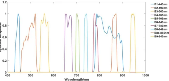
The MSI carried by Sentinel-2A has spectral bands in visible, near infrared and shortwave infrared region, with spatial resolution of 10 m, 20 m and 60 m. There are four bands at 10 m: 490 nm (B2), 560 nm (B3), 665 nm (B4), 842 nm (B8); six bands at 20 m: 705 nm (B5), 740 nm (B6), 783 nm (B7), 865 nm (B8a), 1610 nm (B11), 2190 nm (B12); three bands at 60 m: 443 nm (B1), 945 nm (B9) and 1375 nm (B10). The spectral response functions of Sentinel-2A are used to calculate the band equivalent reflectance by convolving with the simulation data, and then to calculate the broadband vegetation index analyzed in the study. Figure2is the plot of the spectral response functions of bands (B1–B9) in 400–1000 nm. In Section4.2, a brief description of these vegetation indices is presented.
Remote Sens. 2018, 10, x FOR PEER REVIEW 8 of 22
3.2. Sentinel–2A
The goal in our sensitivity analysis is to obtain wavelength relationships that maximize the possibility of retrieving some important parameters in wetland aquatic vegetation areas. These wavelength relationships were compared with the available bands on the broadband sensors such as Sentinel-2A. Macrophytes have complex spatial mosaic structures and, therefore, require concurrent high spatial and spectral resolution remote sensing data. The Sentinel-2A is a twin polar-orbiting satellite mission with wide swath, high spatial and spectral resolution and revisiting frequency that is expected to have significant potential for mapping aquatic vegetation in complex wetland ecosystems [52]. Furthermore, the Multispectral Imager Instrument (MSI) carried on Sentinel-2A has 13 spectral bands, especially four bands that cover the “red edge” region, which is in the range of 700–750 nm. These bands can provide enriched capabilities for the detection of aquatic vegetation. The open access and free-of-charge policy adopted for the Sentinel-2A data products favor routine environmental applications (including wetlands). Therefore, Sentinel-2A is chosen as the reference sensor in this paper, which aims to provide theoretical support for future retrieval of aquatic vegetation parameters in the context of optical remote sensing.
The MSI carried by Sentinel-2A has spectral bands in visible, near infrared and shortwave infrared region, with spatial resolution of 10 m, 20 m and 60 m. There are four bands at 10 m: 490 nm (B2), 560 nm (B3), 665 nm (B4), 842 nm (B8); six bands at 20 m: 705 nm (B5), 740 nm (B6), 783 nm (B7), 865 nm (B8a), 1610 nm (B11), 2190 nm (B12); three bands at 60 m: 443 nm (B1), 945 nm (B9) and 1375 nm (B10). The spectral response functions of Sentinel-2A are used to calculate the band equivalent reflectance by convolving with the simulation data, and then to calculate the broadband vegetation index analyzed in the study. Figure 2 is the plot of the spectral response functions of bands (B1–B9) in 400–1000 nm. In Section 4.2, a brief description of these vegetation indices is presented.
Figure 2. The Sentinel-2A spectral response functions of bands (B1–B9) in 400–1000 nm.
4. Results
4.1. GSA to Reflectance in Different Cases
For the cases set in Section 3.1, the total order sensitivity indices of input parameters are calculated wavelength by wavelength. It can be assumed that if a parameter is highly sensitive over a band range, it will have a significant effect on canopy reflectance over this range, and inversion of the parameter by reflectance in this band range should be possible.
To show clearly the sensitivity of different input parameters at each wavelength, the total order sensitivity indices of all parameters are normalized to the range 0–1, which refers to the contribution of a single parameter to the sum of all parameter’s sensitivity. To evaluate the impact of a single parameter on the reflectance over the whole band range (400–1000 nm), the influence of the parameter
4. Results
4.1. GSA to Reflectance in Different Cases
For the cases set in Section3.1, the total order sensitivity indices of input parameters are calculated wavelength by wavelength. It can be assumed that if a parameter is highly sensitive over a band range, it will have a significant effect on canopy reflectance over this range, and inversion of the parameter by reflectance in this band range should be possible.
To show clearly the sensitivity of different input parameters at each wavelength, the total order sensitivity indices of all parameters are normalized to the range 0–1, which refers to the contribution of a single parameter to the sum of all parameter’s sensitivity. To evaluate the impact of a single parameter on the reflectance over the whole band range (400–1000 nm), the influence of the parameter (PI) is defined as the ratio of the sum of the normalized total order sensitivity (NST) index of the parameter to the sum of all the parameters’NSTover the entire band range:
PIi = 1000 ∑ λ=400 NSTi(λ) 16 ∑ i=1 1000 ∑ λ=400 NSTi(λ) (7)
In Equation (7), PIi stands for the impact of the i-th input parameter, and λ represents the
wavelength, which is in the range of 400–1000 nm.PImeans theNSTproportion of thei-th parameter in all parameters over the whole band range. Next, the analysis results of emergent vegetation and submerged vegetation will be introduced.
4.1.1. Emergent Vegetation
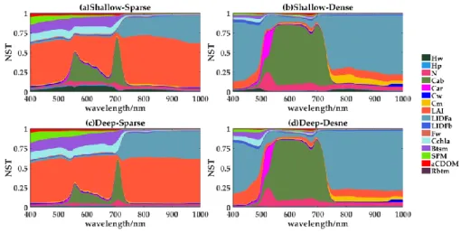
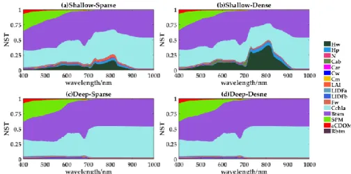
Figure3is the cumulative plot ofNSTfor emergent vegetation in four different cases. The larger area of a parameter in the band range means it is more significant to the reflectance.
Remote Sens. 2018, 10, x FOR PEER REVIEW 9 of 22
(PI) is defined as the ratio of the sum of the normalized total order sensitivity (NST) index of the
parameter to the sum of all the parameters’ NST over the entire band range:
1000 400 16 1000 1 400 i i i i NST PI NST (7)In Equation (7), PIi stands for the impact of the i-th input parameter, and represents the
wavelength, which is in the range of 400–1000 nm. PI means the NST proportion of the i-th parameter
in all parameters over the whole band range. Next, the analysis results of emergent vegetation and submerged vegetation will be introduced.
4.1.1. Emergent Vegetation
Figure 3 is the cumulative plot of NST for emergent vegetation in four different cases. The larger
area of a parameter in the band range means it is more significant to the reflectance.
Figure 3. The cumulative plot of normalized total order sensitivity (NST) for emergent vegetation in
four different cases. (a), (b), (c), (d) represent the cases of shallow-sparse, shallow-dense, deep-sparse and deep-dense, respectively. The area enclosed by the curve and the horizontal axis (the first parameter in the list, Hw), and between the curves (except Hw) represents the value of NST.
Combined with Equation (7), high sensitivity vegetation parameters include N, Cab, Car, Cm, LAI and LIDFa. High sensitivity water parameters include Hp, Cchla, Btsm and SPM. It can be seen from Figure 3 that the sensitivity of vegetation parameters is far greater than that of the water parameters for all four cases defined in this study, especially Cab, LAI and LIDFa. The water parameters score only weakly high sensitivity in sparse cases, and the sensitivity is higher in deep-sparse case (Figure 3c) than shallow-deep-sparse case (Figure 3a). Taking Cchla as an example, the values of PI in (a) and (c) are 0.054 and 0.059 respectively.
Figure 4 shows the high sensitivity parameters in different cases varying with wavelength. Comparing with (a), (b), (c) and (d), the range of depth (shallow or deep) has no significant effect on
the curves of high sensitivity parameters, and it changes the values of NST only in some regions. The
range of LAI (sparse or dense) has an obvious effect on both vegetation and water parameters, which can be partially explained by the vertical structure of emergent vegetation. When emergent vegetation is not too sparse, the water just acts as a background and apparently cannot influence the canopy reflectance.
The high sensitivity vegetation parameters of AVRT can be divided into leaf parameters N, Cab, Car, Cm, and canopy parameters LAI, LIDFa. Figure 4 shows that the sensitivity values of leaf parameters and LIDFa are much greater in dense cases than in sparse cases whereas the sensitivity of LAI is the opposite. In sparse cases, the sensitivity values of N, Car and Cm are almost negligible.
Figure 3.The cumulative plot of normalized total order sensitivity (NST) for emergent vegetation in four different cases. (a), (b), (c), (d) represent the cases of shallow-sparse, shallow-dense, deep-sparse and deep-dense, respectively. The area enclosed by the curve and the horizontal axis (the first parameter in the list, Hw), and between the curves (except Hw) represents the value ofNST.
Combined with Equation (7), high sensitivity vegetation parameters include N, Cab, Car, Cm, LAI and LIDFa. High sensitivity water parameters include Hp, Cchla, Btsm and SPM. It can be seen from Figure3that the sensitivity of vegetation parameters is far greater than that of the water parameters for all four cases defined in this study, especially Cab, LAI and LIDFa. The water parameters score only
weakly high sensitivity in sparse cases, and the sensitivity is higher in deep-sparse case (Figure3c) than shallow-sparse case (Figure3a). Taking Cchla as an example, the values ofPIin (a) and (c) are 0.054 and 0.059 respectively.
Figure4 shows the high sensitivity parameters in different cases varying with wavelength. Comparing with (a), (b), (c) and (d), the range of depth (shallow or deep) has no significant effect on the curves of high sensitivity parameters, and it changes the values ofNSTonly in some regions. The range of LAI (sparse or dense) has an obvious effect on both vegetation and water parameters, which can be partially explained by the vertical structure of emergent vegetation. When emergent vegetation is not too sparse, the water just acts as a background and apparently cannot influence the canopy reflectance.
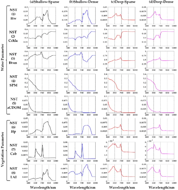
The high sensitivity vegetation parameters of AVRT can be divided into leaf parameters N, Cab, Car, Cm, and canopy parameters LAI, LIDFa. Figure 4shows that the sensitivity values of leaf parameters and LIDFa are much greater in dense cases than in sparse cases whereas the sensitivity of LAI is the opposite. In sparse cases, the sensitivity values of N, Car and Cm are almost negligible. In dense cases, the high sensitivity regions of N and Car are around 510 nm and 500 nm respectively. The region at 500 nm corresponds to the absorption band of Car. The absorption spectrum of Car is also shown in Figure4. The high sensitive range of Cm is mainly around 700–900 nm where the maximum is at 810 nm. The sensitivity of Cm is slightly lower in case (d) than (b) where the maximum ofNSTare 0.073 and 0.111 respectively.
The sensitivity of Cab is very high in the visible region. In sparse cases, theNSTvalues of Cab peak are at 550 nm and 710 nm whereas the trough is at 670 nm. The values in shallow cases are slightly higher than those in deep cases, where the maxima are 0.577 and 0.505 in (a) and (c), respectively. In dense cases, the sensitivity of Cab is very high in the range of 550–750 nm while the trough near 670 nm is no longer obvious. The values ofNSTwithin this range are kept at about 0.755, which shows negligible response to the change in water depth. In general, it can be summarized from the above analysis that the greatest sensitivity to Cab exists in three characteristic bands located at 550 nm, 670 nm and 710 nm. The absorption spectrum of Cab is also shown in Figure4, where it can be seen that the trough is located at 550 nm while the peak is at 670 nm. Besides, the “red edge” position of the vegetation canopy spectrum is located at 710 nm. Thus, the optical properties of chemical substances in the leaves, such as Car and Cab, show up well in GSA.
LAI and Leaf Angle Distribution (LAD) are the two significant parameters that mainly control the amount of light interception and dominate the canopy reflectance for terrestrial vegetation in the visible and NIR regions. LAI can be treated as an important factor for assessing the growth status and biomass. LIDFa and LIDFb are adopted to describe LAD in AVRT model. The former controls the average leaf slope and the latter controls the bimodality distribution of leaves. According to Figure4, the sensitivity values of LAI and LIDFa are strongly affected by the extent of vegetation cover. In sparse cases, theNSTvalues of LAI are very significant within the range of 400–500 nm, 650–680 nm and 730–1000 nm whereas the troughs are around 550 nm and 710 nm. It can be considered that theNST values of LAI and Cab are negatively correlated. The maximumNSTof LAI is about 0.5–0.6 in (a) and (c), which is almost unaffected by the variation of water depth. The range of influence of LIDFa is 730–1000 nm, and the maximum ofNSTis about 0.3–0.4 in (a) and (c). The value ofNSTis close to zero in the visible range. In dense cases, the sensitivity of LAI declines abruptly to around 0.1–0.2, especially in 400–500 nm and 650–680 nm. On the contrary, the sensitivity of LIDFa increases strongly, especially in 400–500 nm and 730–1000 nm with a maximumNSTof 0.765 in (b) and 0.755 in (d). The sensitivity of LIDFa is relatively low near 500–710 nm, due to the high sensitivity of Cab in this range.
The sensitivity values of water parameters in dense cases are almost negligible. In sparse cases, the sensitive ranges of Cchla and Btsm are mainly in the visible band of 400–700 nm, and the range of influence of SPM is mainly in 400–500 nm. Their maxima values ofNSTare all around 0.1–0.2.
Remote Sens.2018,10, 837 11 of 22
In dense cases, the high sensitivity regions of N and Car are around 510 nm and 500 nm respectively. The region at 500 nm corresponds to the absorption band of Car. The absorption spectrum of Car is also shown in Figure 4. The high sensitive range of Cm is mainly around 700–900 nm where the maximum is at 810 nm. The sensitivity of Cm is slightly lower in case (d) than (b) where the maximum of NST are 0.073 and 0.111 respectively.
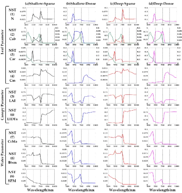
Figure 4. In four different cases, the curves of high sensitivity parameters varying with wavelength.
The columns (a), (b), (c), (d) represent the case of shallow-sparse, shallow-dense, deep-sparse and deep-dense, respectively. (1)–(9) represent the high sensitivity parameters, (1): N, (2): Concentration of chlorophyll a + b (Cab), (3): Concentration of carotenoid (Car), (4): Concentration of dry matter (Cm), (5): Leaf area index (LAI), (6): Leaf inclination distribution function parameter a (LIDFa), (7): Concentration of chlorophyll a, in water (Cchla), (8): Coefficient to calculate scattering of total suspended matter (Btsm), (9): Concentration of suspended matter (SPM). It should be noted that the curves of absorption coefficient of Cab and Car are also shown in (2) and (3). The vertical axis on the right shows the range of the absorption coefficient.
The sensitivity of Cab is very high in the visible region. In sparse cases, the NST values of Cab
peak are at 550 nm and 710 nm whereas the trough is at 670 nm. The values in shallow cases are slightly higher than those in deep cases, where the maxima are 0.577 and 0.505 in (a) and (c), respectively. In dense cases, the sensitivity of Cab is very high in the range of 550–750 nm while the
trough near 670 nm is no longer obvious. The values of NST within this range are kept at about 0.755,
which shows negligible response to the change in water depth. In general, it can be summarized from
Figure 4.In four different cases, the curves of high sensitivity parameters varying with wavelength. The columns (a), (b), (c), (d) represent the case of shallow-sparse, shallow-dense, deep-sparse and deep-dense, respectively. (1)–(9) represent the high sensitivity parameters, (1): N, (2): Concentration of chlorophyll a + b (Cab), (3): Concentration of carotenoid (Car), (4): Concentration of dry matter (Cm), (5): Leaf area index (LAI), (6): Leaf inclination distribution function parameter a (LIDFa), (7): Concentration of chlorophyll a, in water (Cchla), (8): Coefficient to calculate scattering of total suspended matter (Btsm), (9): Concentration of suspended matter (SPM). It should be noted that the curves of absorption coefficient of Cab and Car are also shown in (2) and (3). The vertical axis on the right shows the range of the absorption coefficient.
4.1.2. Submerged Vegetation
The GSA results of submerged vegetation are presented next: they are clearly different from the results for emergent vegetation. Figure5is the cumulative plot ofNSTfor submerged vegetation for four different cases. According to GSA, the high sensitivity water parameters include Hw, Cchla, Btsm, SPM and aCDOM, and the high sensitivity vegetation parameters include Hp, Cab and LAI.
Unlike emergent vegetation, the sensitivity values of water parameters are far greater than those of vegetation parameters, especially Cchla and Btsm, both of which are highly sensitive over the entire band range (Figure5). In the case of (a) (shallow-sparse), for example, thePIvalues of these two parameters are 0.388 and 0.428, respectively, while the most sensitive vegetation parameter LAI
Remote Sens.2018,10, 837 12 of 22
scores only 0.012. In deep cases, the effects of vegetation parameters are almost obscured by water parameters, even in deep-dense case. No matter what case, the sensitivity of bottom reflectance is almost negligible. The variation of sensitivity is fully investigated in Figure6, which shows the curves of high sensitivity parameters in different cases varying with wavelength.
the above analysis that the greatest sensitivity to Cab exists in three characteristic bands located at 550 nm, 670 nm and 710 nm. The absorption spectrum of Cab is also shown in Figure 4, where it can be seen that the trough is located at 550 nm while the peak is at 670 nm. Besides, the “red edge” position of the vegetation canopy spectrum is located at 710 nm. Thus, the optical properties of chemical substances in the leaves, such as Car and Cab, show up well in GSA.
LAI and Leaf Angle Distribution (LAD) are the two significant parameters that mainly control the amount of light interception and dominate the canopy reflectance for terrestrial vegetation in the visible and NIR regions. LAI can be treated as an important factor for assessing the growth status and biomass. LIDFa and LIDFb are adopted to describe LAD in AVRT model. The former controls the average leaf slope and the latter controls the bimodality distribution of leaves. According to Figure 4, the sensitivity values of LAI and LIDFa are strongly affected by the extent of vegetation
cover. In sparse cases, the NST values of LAI are very significant within the range of 400–500 nm,
650–680 nm and 730–1000 nm whereas the troughs are around 550 nm and 710 nm. It can be
considered that the NST values of LAI and Cab are negatively correlated. The maximum NST of LAI
is about 0.5–0.6 in (a) and (c), which is almost unaffected by the variation of water depth. The range
of influence of LIDFa is 730–1000 nm, and the maximum of NST is about 0.3–0.4 in (a) and (c). The
value of NST is close to zero in the visible range. In dense cases, the sensitivity of LAI declines abruptly to around 0.1–0.2, especially in 400–500 nm and 650–680 nm. On the contrary, the sensitivity
of LIDFa increases strongly, especially in 400–500 nm and 730–1000 nm with a maximum NST of
0.765 in (b) and 0.755 in (d). The sensitivity of LIDFa is relatively low near 500–710 nm, due to the high sensitivity of Cab in this range.
The sensitivity values of water parameters in dense cases are almost negligible. In sparse cases, the sensitive ranges of Cchla and Btsm are mainly in the visible band of 400–700 nm, and the range
of influence of SPM is mainly in 400–500 nm. Their maxima values of NST are all around 0.1–0.2.
4.1.2. Submerged Vegetation
The GSA results of submerged vegetation are presented next: they are clearly different from the
results for emergent vegetation. Figure 5 is the cumulative plot of NST for submerged vegetation for
four different cases. According to GSA, the high sensitivity water parameters include Hw, Cchla, Btsm, SPM and aCDOM, and the high sensitivity vegetation parameters include Hp, Cab and LAI.
Figure 5. The cumulative plot of NST for submerged vegetation in four different cases. (a), (b), (c), (d)
represent the cases of shallow-sparse, shallow-dense, deep-sparse and deep-dense, respectively. The area enclosed by the curve and the horizontal axis (the first parameter in the list, Hw), and between the curves (except Hw) represents the value of NST.
Unlike emergent vegetation, the sensitivity values of water parameters are far greater than those of vegetation parameters, especially Cchla and Btsm, both of which are highly sensitive over the
entire band range (Figure 5). In the case of (a) (shallow-sparse), for example, the PI values of these
Figure 5.The cumulative plot ofNSTfor submerged vegetation in four different cases. (a), (b), (c), (d) represent the cases of shallow-sparse, shallow-dense, deep-sparse and deep-dense, respectively. The area enclosed by the curve and the horizontal axis (the first parameter in the list, Hw), and between the curves (except Hw) represents the value ofNST.
The influence ranges of SPM and aCDOM are relatively narrow, with the decreasing trend of NSTat 400–600 nm and 400–550 nm, respectively. The sensitivity values of SPM and aCDOM in deep cases are slightly greater than those in shallow cases. Hw is more sensitive in shallow cases than in deep cases, and the values ofPIin these cases are 0.055, 0.124, 0.003 and 0.004 respectively, indicating that the influence of Hw on the canopy reflectance could not be significant when the water depth increases to a certain extent. The curves of Hw have different patterns in shallow and deep cases. In shallow cases, the influence range of Hw is mainly located in 700–900 nm, while in deep cases it changes to 500–700 nm, the peak being at 600 nm. Hw is more sensitive in dense cases than in sparse cases, indicating that the increase of water depth will make the attenuation more obvious in dense cases than sparse cases.
In either case, Cchla and Btsm have very significant effects over the whole band range. They have different influence ranges in shallow and deep cases. The sensitivity values in deep cases are slightly higher than those in shallow cases. Taking Cchla as an example,PIis 0.388, 0.347, 0.403 and 0.404 in these four cases, respectively. In shallow cases, the curve of Cchla has a minor trough around 680 nm and 810 nm, while the peak of Btsm’s curve is near 680 nm. In deep cases, there are similar relationships between Cchla and Btsm, indicating that it would be helpful for constructing the inversion algorithm by using the bands around 680 nm to suppress the impact of Btsm. Currently, this band has been applied to construct the three-band [53] and four-band [54] semi-analytical method to extract the concentration of chlorophyll in high-turbidity water.
The sensitivity features of vegetation parameters deserve more attention: they can provide the theoretical basis for inversion of submerged vegetation parameters. Relative to shallow cases, theNST values of vegetation parameters are much lower in deep cases, since the increase of water depth means the canopy signal will be attenuated more strongly. The sensitivity values of Hp are slightly lower than those of LAI and Cab, and the values ofPIin four cases are 0.016, 0.020, 0.004 and 0.003, respectively. The curve of Hp has no stable shape because it does not directly reflect the biophysical-biochemical properties of the plant. It mainly reflects the vertical height of the water-vegetation mixed medium in the model. In general, its influence range is located in 700–900 nm in shallow cases.
Remote Sens.2018,10, 837 13 of 22
two parameters are 0.388 and 0.428, respectively, while the most sensitive vegetation parameter LAI scores only 0.012. In deep cases, the effects of vegetation parameters are almost obscured by water parameters, even in deep-dense case. No matter what case, the sensitivity of bottom reflectance is almost negligible. The variation of sensitivity is fully investigated in Figure 6, which shows the curves of high sensitivity parameters in different cases varying with wavelength.
Figure 6. In four different cases, the curves of high sensitivity parameters varying with wavelength.
The columns (a), (b), (c), (d) represent the case of shallow-sparse, shallow-dense, deep-sparse and deep-dense, respectively. (1)–(9) represent the high sensitivity parameters of the model, (1): The height of the upper water layer (Hw), (2): Concentration of chlorophyll a, in water (Cchla), (3): Coefficient to calculate scattering of total suspended matter (Btsm), (4): Concentration of suspended matter (SPM), (5): Absorption coefficient of CDOM at 375 nm (aCDOM), (6): Plant height (Hp), (7): Concentration of chlorophyll a+b (Cab), (8): Leaf area index (LAI).
The influence ranges of SPM and aCDOM are relatively narrow, with the decreasing trend of
NST at 400–600 nm and 400–550 nm, respectively. The sensitivity values of SPM and aCDOM in deep
cases are slightly greater than those in shallow cases. Hw is more sensitive in shallow cases than in deep cases, and the values of PI in these cases are 0.055, 0.124, 0.003 and 0.004 respectively, indicating that the influence of Hw on the canopy reflectance could not be significant when the water depth increases to a certain extent. The curves of Hw have different patterns in shallow and deep cases. In
Figure 6.In four different cases, the curves of high sensitivity parameters varying with wavelength. The columns (a), (b), (c), (d) represent the case of shallow-sparse, shallow-dense, deep-sparse and deep-dense, respectively. (1)–(9) represent the high sensitivity parameters of the model, (1): The height of the upper water layer (Hw), (2): Concentration of chlorophyll a, in water (Cchla), (3): Coefficient to calculate scattering of total suspended matter (Btsm), (4): Concentration of suspended matter (SPM), (5): Absorption coefficient of CDOM at 375 nm (aCDOM), (6): Plant height (Hp), (7): Concentration of chlorophyll a+b (Cab), (8): Leaf area index (LAI).
The sensitivity patterns of Cab and LAI are stable, especially Cab. The bands around 550 nm and 710 nm are high sensitivity regions of Cab, while the other regions have almost no sensitivity, which is similar to the result of 4.1.1. However, the GSA results for LAI are slightly different from the conclusion in 4.1.1. In shallow cases, the influence range of LAI is 700–900 nm while theNSTvalues are much smaller in the shallow-dense case. For deep cases, its influence shifts to around 500 nm, and theNSTvalues drop to the order of 10−3, which cannot provide useful information. As with the above results, Cab is more sensitive in dense cases than in sparse cases, while LAI is more sensitive in sparse cases than in dense cases.
The inversion methods of vegetation parameters are usually based on the vegetation index, which is a common tool for the terrestrial vegetation remote sensing. In the following, the GSA will be performed on the vegetation index.
4.2. GSA to VIs in Different Cases
This section will discuss the GSA results for the high sensitivity parameters to vegetation index identified in 4.1. Vegetation index refers to the band combinations of satellite data. Huete et al. pointed out that the purpose of constructing VI is to enhance the vegetation signal while weakening the impact resulting from the background [55], which makes it an effective approach for inversion. Around this goal, many scholars have constructed various forms of vegetation indices, such as NDVI [56], PVI [56], SAVI [57], and EVI [58].
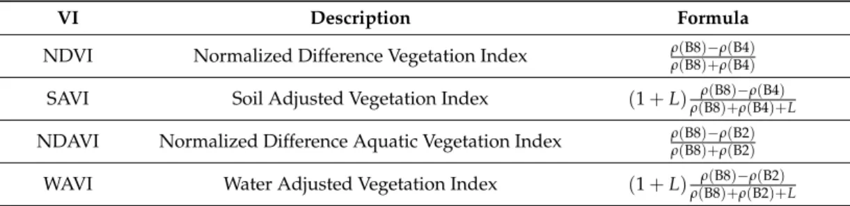
In Section 4.1, many emergent vegetation and submerged vegetation canopy spectra under different input conditions have been simulated. The canopy spectra are convolved with the spectral response functions of Sentinel-2A to obtain the band equivalent reflectance, and then to enable the vegetation index to be calculated. The sensitivity of model input parameters to vegetation indices can be obtained by EFAST. Table2summarizes the formulae of vegetation indices to be analyzed. The bands in the formulae are represented by the band numbers in Section3.2. For example, B2 indicates the second band of Sentinel-2A (blue band). The value ofLfor both SAVI and WAVI is 0.5. It should be pointed out that the spatial resolution of all the bands selected in the formulae is 10 m. Although there are other bands with narrower band width in the similar band range (such as B6 and B7, which also locate in the near infrared band), the mixing-pixel problems in wetland remote sensing are more complicated, which means bands with high spatial resolution hold more advantages.
Table 2.The formulae of vegetation indices to be analyzed.
VI Description Formula
NDVI Normalized Difference Vegetation Index ρ(B8)−ρ(B4) ρ(B8)+ρ(B4)
SAVI Soil Adjusted Vegetation Index (1+L) ρ(B8)−ρ(B4) ρ(B8)+ρ(B4)+L NDAVI Normalized Difference Aquatic Vegetation Index ρ(B8)−ρ(B2)
ρ(B8)+ρ(B2) WAVI Water Adjusted Vegetation Index (1+L) ρ(B8)−ρ(B2)
ρ(B8)+ρ(B2)+L
4.2.1. Emergent Vegetation
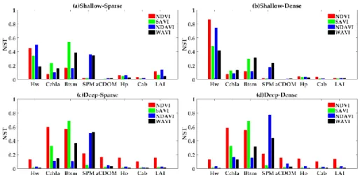
Figure7is the column chart ofNSTvalues to vegetation indices mentioned above in four different cases for emergent vegetation. The high sensitivity parameters presented in the chart are the same as those in 4.1.1. The analysis results shown in Figure7are similar to those shown in Figure4. In sparse cases, LAI is the most sensitive parameter to all vegetation indices, indicating that it is possible to retrieve LAI in sparse cases rather than dense cases via the vegetation index. Whereas the sensitivity of LAI in dense cases is weakened, just like that in Figure4. The sensitivity of leaf parameters such as Cab and Car, and LIDFa rises strongly. In case (a) the sensitivity of LAI to NDAVI is greater than to the other indices, and the values ofNSTare 0.572, 0.805, 0.893 and 0.830 respectively. It can be attributed to the fact that the formulae of those indices all contain the near infrared (B8) band, which is the sensitive band of LAI in sparse cases according to Figure4. However, NDAVI and WAVI, which are formulated by the blue band (B2), perform better than NDVI and SAVI formulated by the red band (B4) because LAI is more sensitive in the blue band than that in the red band. In fact, except for case (c), theNSTof LAI to NDAVI is higher than to the other indices, which indicates that for emergent vegetation, NDAVI is more suitable for LAI inversion than the other indices except the deep-sparse case. This result is consistent with the conclusion of Villa et al. that for aquatic vegetation LAI is more sensitive to NDAVI than to the conventional terrestrial vegetation index [38]. In case (c), LAI scores higher sensitivity to
Remote Sens.2018,10, 837 15 of 22
NDVI, indicating that NDVI is a better option in deep-sparse case. The sensitivity of LAI to NDAVI in (c) is the lowest, probably due to the combined effect of increased water depth and water parameters in the blue band.
Table 2. The formulae of vegetation indices to be analyzed.
VI Description Formula
NDVI Normalized Difference Vegetation Index
B8 - B4 B8 + B4 SAVI Soil Adjusted Vegetation Index
1+
B8 - B4B8 + B4 +
L
L
NDAVI Normalized Difference Aquatic Vegetation Index
B8 B2 B8 B2 WAVI Water Adjusted Vegetation Index
1+
B8 - B2B8 + B2 +
L
L
4.2.1. Emergent Vegetation
Figure 7 is the column chart of NST values to vegetation indices mentioned above in four different cases for emergent vegetation. The high sensitivity parameters presented in the chart are the same as those in 4.1.1. The analysis results shown in Figure 7 are similar to those shown in Figure 4. In sparse cases, LAI is the most sensitive parameter to all vegetation indices, indicating that it is possible to retrieve LAI in sparse cases rather than dense cases via the vegetation index. Whereas the sensitivity of LAI in dense cases is weakened, just like that in Figure 4. The sensitivity of leaf parameters such as Cab and Car, and LIDFa rises strongly. In case (a) the sensitivity of LAI to NDAVI is greater than to the other indices, and the values of NST are 0.572, 0.805, 0.893 and 0.830 respectively. It can be attributed to the fact that the formulae of those indices all contain the near infrared (B8) band, which is the sensitive band of LAI in sparse cases according to Figure 4. However, NDAVI and WAVI, which are formulated by the blue band (B2), perform better than NDVI and SAVI formulated by the red band (B4) because LAI is more sensitive in the blue band than that in the red band. In fact,
except for case (c), the NST of LAI to NDAVI is higher than to the other indices, which indicates that
for emergent vegetation, NDAVI is more suitable for LAI inversion than the other indices except the deep-sparse case. This result is consistent with the conclusion of Villa et al. that for aquatic vegetation LAI is more sensitive to NDAVI than to the conventional terrestrial vegetation index [38]. In case (c), LAI scores higher sensitivity to NDVI, indicating that NDVI is a better option in deep-sparse case. The sensitivity of LAI to NDAVI in (c) is the lowest, probably due to the combined effect of increased water depth and water parameters in the blue band.
Figure 7. The NST of high sensitivity parameters to vegetation indices for emergent vegetation. (a),
(b), (c), (d) represent the case of shallow-sparse, shallow-dense, deep-sparse and deep-dense, respectively.
Figure 7.TheNSTof high sensitivity parameters to vegetation indices for emergent vegetation. (a), (b), (c), (d) represent the case of shallow-sparse, shallow-dense, deep-sparse and deep-dense, respectively.
In dense cases, the sensitivity of leaf parameters increases clearly, especially for Cab. The sensitivity of Cab to NDVI is much higher than that to the other indices. In case (b), theNST of Cab is 0.842, 0.090, 0.158 and 0.010, respectively, since NDVI is constructed by the red and near infrared bands, which are the trough and peak respectively in Figure4, and both of these bands are characteristic. Car is more sensitive to NDAVI than to the other indices due to the high sensitivity in the blue band. As for LIDFa, its sensitivity to the adjusted indices (WAVI and SAVI) is much higher than that to the normalized indices (NDAVI and WAVI), which are constructed by the same band combinations. Taking case (b) as an example, theNSTof LIDFa are 0.059, 0.590, 0.199 and 0.700, respectively. This could be a result of the adjustment factorL.
There is almost no sensitivity of the water parameters to the vegetation indices, which is plausible since the vegetation index is designed to enhance the contribution of vegetation properties and canopy structural variations, at the same time reducing background (soil and water) effects.
4.2.2. Submerged Vegetation
The following are the GSA results for submerged vegetation. Figure8is the column chart of NSTvalues to vegetation indices in four above-defined cases. In shallow-sparse case, all the water parameters are sensitive to one or several vegetation indices. Taking SPM as an example, it is sensitive to NDAVI and WAVI. In shallow-dense case, Hw is the most sensitive parameter to all indices, since all the indices have near infrared bands, where the sensitivity of Hw is much higher than the other parameters according to Figure5. The other water parameters are less sensitive to vegetation indices, which could be explained by the lower sensitivity to reflectance in the near infrared region. Among the vegetation parameters, the sensitivities of Hp and Cab are insignificant, whereas LAI is sensitive only to the four indices in case (a), to some degree, which is consistent with the results in Figure5. In case (a), the sensitivity of LAI to NDAVI is higher than to the other indices, and theNSTvalues of LAI to all four indices are 0.115, 0.066, 0.141 and 0.049, respectively, which is similar to the results of Villa et al. as well [38].
Remote Sens.2018,10, 837 16 of 22
In dense cases, the sensitivity of leaf parameters increases clearly, especially for Cab. The
sensitivity of Cab to NDVI is much higher than that to the other indices. In case (b), the NST of Cab
is 0.842, 0.090, 0.158 and 0.010, respectively, since NDVI is constructed by the red and near infrared bands, which are the trough and peak respectively in Figure 4, and both of these bands are characteristic. Car is more sensitive to NDAVI than to the other indices due to the high sensitivity in the blue band. As for LIDFa, its sensitivity to the adjusted indices (WAVI and SAVI) is much higher than that to the normalized indices (NDAVI and WAVI), which are constructed by the same band combinations. Taking case (b) as an example, the NST of LIDFa are 0.059, 0.590, 0.199 and 0.700, respectively. This could be a result of the adjustment factor L.
There is almost no sensitivity of the water parameters to the vegetation indices, which is plausible since the vegetation index is designed to enhance the contribution of vegetation properties and canopy structural variations, at the same time reducing background (soil and water) effects. 4.2.2. Submerged Vegetation
The following are the GSA results for submerged vegetation. Figure 8 is the column chart of NST
values to vegetation indices in four above-defined cases. In shallow-sparse case, all the water parameters are sensitive to one or several vegetation indices. Taking SPM as an example, it is sensitive to NDAVI and WAVI. In shallow-dense case, Hw is the most sensitive parameter to all indices, since all the indices have near infrared bands, where the sensitivity of Hw is much higher than the other parameters according to Figure 5. The other water parameters are less sensitive to vegetation indices, which could be explained by the lower sensitivity to reflectance in the near infrared region. Among the vegetation parameters, the sensitivities of Hp and Cab are insignificant, whereas LAI is sensitive only to the four indices in case (a), to some degree, which is consistent with the results in Figure 5. In
case (a), the sensitivity of LAI to NDAVI is higher than to the other indices, and the NST values of
LAI to all four indices are 0.115, 0.066, 0.141 and 0.049, respectively, which is similar to the results of Villa et al. as well [38].
Figure 8. The NST of high sensitivity parameters to vegetation indices for submerged vegetation. (a),
(b), (c), (d) represent the cases of shallow-sparse, shallow-dense, deep-sparse and deep-dense, respectively.
However, in deep cases Hw is sensitive only to NDVI while the sensitivity values of the other water parameters rise substantially. SPM is highly sensitive to NDAVI and to WAVI since they both utilize the blue band, which is exactly in the high sensitivity range of SPM. Btsm shows higher
sensitivity to SAVI and WAVI than to NDVI and NDAVI, probably due to the adjustment factor L.
In fact, Hw is less sensitive to the adjusted vegetation indices in four cases, which means L does
effectively suppress the influence of water depth, but it seems that L cannot suppress the effects of
water constituent parameters, especially Cchla and Btsm. Considering that the sensitivity values of these two parameters to reflectance over the whole band range are far too significant, especially in
Figure 8. The NST of high sensitivity parameters to vegetation indices for submerged vegetation. (a), (b), (c), (d) represent the cases of shallow-sparse, shallow-dense, deep-sparse and deep-dense, respectively.
However, in deep cases Hw is sensitive only to NDVI while the sensitivity values of the other water parameters rise substantially. SPM is highly sensitive to NDAVI and to WAVI since they both utilize the blue band, which is exactly in the high sensitivity range of SPM. Btsm shows higher sensitivity to SAVI and WAVI than to NDVI and NDAVI, probably due to the adjustment factorL. In fact, Hw is less sensitive to the adjusted vegetation indices in four cases, which meansL does effectively suppress the influence of water depth, but it seems thatLcannot suppress the effects of water constituent parameters, especially Cchla and Btsm. Considering that the sensitivity values of these two parameters to reflectance over the whole band range are far too significant, especially in deep cases, it is difficult to find the suitable bands to resist the sensitivity of Cchla and Btsm. In cases (c) and (d), although theNSTvalues of vegetation parameters are too low, it should still be pointed out that the sensitivity values of LAI and Cab to NDVI are much higher than to the other indices. Taking (c) as an example, theNSTof LAI to the indices are 0.151, 0.017, 0.023 and 0.016, respectively. As for Cab, the values are 0.100, 0.012, 0.014 and 0.010, respectively. These results may provide clues for species identification and vegetation parameters inversion for submerged vegetation.
5. Discussion
According to the results in Section4, the influential variables of the coupled macrophyte-water system, and the conditions under which they are sensitive, can be revealed, givena prioriknowledge in the inversion of parameters. For example, it can be seen from Figure4that LAI scores high sensitivity around 650–680 nm and 730–1000 nm for emergent vegetation in sparse cases. These two band ranges have been utilized to build many vegetation indices such as NDVI and SAVI, which have greatly helped retrieval of LAI for terrestrial vegetation. Therefore, the high sensitivity of LAI around 700–900 nm (Figure6) is expected to provide clues for the inversion of LAI for submerged vegetation in shallow-sparse case.
For emergent vegetation, its canopy reflectance is dominated by vegetation parameters, which is similar to the case for terrestrial vegetation. The inversion of LAI will be possible when the vegetation is sparse, while the inversion of the leaf parameters such as Cab is possible in dense cases. The bands around 550 nm and 710 nm are peaks for Cab and troughs for LAI, and the band around 670 nm is a trough for Cab and a peak for LAI, giving suitable conditions for constructing inversion algorithms. These bands have been fully utilized in terrestrial vegetation remote sensing. The above results indicate that it will be a major challenge in wetland remote sensing to distinguish emergent vegetation growing in near shore with terrestrial vegetation [59]. The results for vegetation indices are consistent with those to reflectance in some degree. The sensitivity of LAI to indices is high