these trends have also led to an increase in power consumption that is becoming a key limiting factor in the design of such scalable interconnected systems. Power-aware networks, therefore, need to become inherent components of single and multi-chip parallel systems. In the hardware arena, recent interconnection network power-management research work has employed limited-scope techniques that mostly focus on reducing the power consumed by the network communi-cation links. As these limited-scope techniques are not tailored to the applicommuni-cations running on the network, power savings and the corresponding impact on network latency vary significantly from one application to the next as we demonstrate in this paper; in many cases, network per-formance can severely suffer. In the software arena, extensive research on compile-time optimiza-tions has produced parallelizing compilers that can efficiently map an application onto hardware for high performance. However, research into power-aware parallelizing compilers is in its in-fancy. In this paper, we take the first steps toward tailoring applications’ communication needs at run-time for low power. We propose software techniques that extend the flow of a parallelizing Extension of Conference Paper. Original work appeared in CASES’05 [Soteriou et al. 2005]. The extensions found in the journal paper submission are the following:
– Updated Related Work in Section 2.1.
– Addition of method for generating software directives under adaptive routing, along with a detailed mathematical model, Sections 4.1 and 4.1.1.
– Characterization and rationale for the use of buffer utilizations at run-time in concert with software directives, Section 5.1.
– Explanation of how buffer utilization is used in adaptive routing Section 5.2.
– Additional results with adaptive routing in Section 6 for all 28 applications of the three archi-tectures considered.
– Full range of power-performance results (all 28 applications) under traffic perturbation in Sec-tion 6.6, along with updated relevant discussion. The original conference paper only had a subset of these results.
Authors’ address: Vassos Soteriou, Noel Eisley, and Li-Shiuan Peh, Department of Electrical Engineering, Princeton University, Princeton, New Jersey 08544; email: {soteriou,eisley,peh} @princeton.edu.
Permission to make digital or hard copies of part or all of this work for personal or classroom use is granted without fee provided that copies are not made or distributed for profit or direct commercial advantage and that copies show this notice on the first page or initial screen of a display along with the full citation. Copyrights for components of this work owned by others than ACM must be honored. Abstracting with credit is permitted. To copy otherwise, to republish, to post on servers, to redistribute to lists, or to use any component of this work in other works requires prior specific permission and/or a fee. Permissions may be requested from Publications Dept., ACM, Inc., 2 Penn Plaza, Suite 701, New York, NY 10121-0701 USA, fax+1 (212) 869-0481, or [email protected].
C
2007 ACM 1544-3566/2007/03-ART5 $5.00 DOI 10.1145/1216544.1216548 http://doi.acm.org/ 10.1145/1216544.1216548
compiler in order to direct run-time network power reduction. We target network links, a sig-nificant power consumer in these systems, allowing dynamic voltage scaling (DVS) instructions extracted during static compilation to orchestrate link voltage and frequency transitions for power savings during application run-time. Concurrently, an online hardware mechanism measures net-work congestion levels and adapts these off-line DVS settings to maximize netnet-work performance. Our simulations over three existing parallel systems, ranging from very fine-grained single-chip to coarse-grained multi-chip architectures, show that link power consumption can be reduced by up to 76.3%, with a minor increase in latency, ranging from 0.18 to 6.78% across a number of benchmark suites.
Categories and Subject Descriptors: B.9.1 [Power Management]: Low-Power Design [B.8.2 [Per-formance and Reliability]: Per[Per-formance Analysis and Design Aids]: C.2.0 [Computer-Communication Networks]: General
General Terms: Design, Management, Performance
Additional Key Words and Phrases: Software-directed power reduction, dynamic voltage scaling, interconnection networks, on-chip networks, communication links, simulation
ACM Reference Format:
Soteriou, V., Eisley, N., and Peh, L.-S. 2007. Software-directed power-aware interconnection networks. ACM Trans. Architec. Code Optim. 5, 1, Article 5 (March 2007), 40 pages. DOI = 10.1145/1216544.1216548 http://doi.acm.org/10.1145/1216544.1216548.
1. INTRODUCTION
Interconnection networks are becoming thede facto communication fabric in both single-chip multiprocessors (CMPs) [Taylor et al. 2004; Sankaralingam et al. 2003; Dally and Towles 2001] and multi-chip systems [InfiniBand 2006; Mukherjee et al. 2002], facilitating program parallelism as a means to reduce execution time and to achieve very high, scalable performance. While rapidly improving VLSI technology is allowing the use of additional chip resources along with higher clock rates, performance gains do not arrive without cost. As in the case of uniprocessor systems, interconnected systems, both in the on-chip and chip-to-chip domains, suffer from the effects of ever increasing power con-sumption, with the interconnection network taking up a sizable portion of the parallel system’s power budget. For instance, the on-chip network in the MIT Raw CMP consumes 36% of the entire chip’s power budget [Kim et al. 2003]. In board-to-board and multi-chip networks the routers and communication links are already consuming substantial power. In a Mellanox server blade the router and links are estimated to dissipate 15 W out of the total budget of 40 W (37.5%), with the processor allocated the same power budget of 15 W [Mellanox 2006], while 65% of the power budget of the IBM 8-port 12X switch [InfiniBand 2006] is taken up by the communication links (each of the eight ports interfaces 12 2.5 Gbps links that dissipate 2.5 W each, with the entire switch consuming 31 W, on average). In addition, the on-chip router and links of the Alpha 21364 proces-sor consume a substantial 23 W, where the links consume 58% of this allocated power [Mukherjee et al. 2002]. Indeed, the International Technology Roadmap for Semiconductors [ITRS 2005] highlights system power consumption as the limiting factor in developing systems below the 50 nm technology point. To help overcome this barrier, the design of interconnection networks must emphasize power awareness.
link according to the projected traffic levels. Though these approaches are sim-ple and provide good power savings, their limited-scope nature cannot accom-modate the fluctuating link bandwidth needs of a specific application. As Sec-tion 2.2 demonstrates, network performance can be highly variable and unpre-dictable from one application to the next and, in some cases, severely degraded. In the software arena, extensive research on compile-time optimizations has produced heavily optimized compilers [Robert et al. 1996; Lee et al. 1998] that expose program parallelism to efficiently map an application onto the parallel architecture, showing good potential for application execution speedup. How-ever, compiler optimizations that address power issues in parallel architectures remain very limited, with recent work in Kadayif et al. [2004] targeting proces-sor power optimization for array-based applications. In short, communication power reduction at the software level must be addressed more thoroughly.
In this paper we take the first steps toward tailoring applications’ com-munication needs at run-time for low power and propose a software-based methodology that extends the parallel compiler flow in order to construct high-performance power-aware interconnection networks by targeting commu-nication links, a significant power consumer in interconnection networks. Our methodology consumes the statically compiled message flow of an application and analyzes the traffic levels for all links in the network over periods of time. By factoring in architecture characteristics, our technique matches DVS link transitions to the expected levels of traffic, generating DVS software directives that are injected into the network along with the network-mapped application. These DVS instructions are then executed at run-time, dynamically adapting link power consumption to actual utilization. Concurrently, a hardware online mechanism measures network congestion levels and fine-tunes the execution of these DVS instructions to handle run-time variabilities that are not precisely captured at compile-time. Our results show that our software-directed approach demonstrates significantly improved power-performance as compared to prior hardware-based approaches reducing link power by up to 76.3% relative to the baseline network configuration, i.e., without DVS links. Network performance incurs a minor increase in network latency ranging from 0.18 to 6.78% across a number of benchmark suites running on three existing networks, spanning very fine-grained single-chip to coarse-grained multi-chip parallel architectures.
Next, Section 2 discusses prior related research, demonstrating the limited-scope nature of existing hardware-driven approaches and motivates the use of software directives to reduce network power, while Section 3 describes the
assumed DVS link model. Section 4 follows with details of our proposed tech-niques for extracting DVS software directives and Section 5 describes our online DVS hardware mechanism. Section 6 details our simulation setup and results for a range of benchmark suites running on three existing network architec-tures. Finally, Section 7 concludes the paper.
2. BACKGROUND AND MOTIVATION 2.1 Related Work
As parallel systems become faster and increasingly interconnected, there has been increasing recognition of the need to target the power consumption of the interconnection networks employed by these parallel systems. Several recent studies have modeled and characterized the power profile of network routers and links in a variety of systems. Results over a range of configurations, from clusters [Kim et al. 2003] to servers [Patel et al. 1997] and CMPs [Benini and Micheli 2001; Kim et al. 2003; Wang et al. 2002], emphasize and demonstrate the high power consumed by network routers and communication links.
To a limited extent, prior research has explored the use of power-aware methodologies to reduce link power consumption in interconnection networks. Here we categorize them intohardware- andsoftware-basedpower-aware tech-niques. Hardware-based approaches are further arranged into two main classes according to the type of power-aware link mechanism they employ: dynamic voltage scalable (DVS) and on/off links. The first power-aware interconnection networks proposed by Shang et al. [2002] explored the use of DVS links, where hardware counters measure the levels of past and current network utilization over fixed sampling windows. These online statistics are then compared to fixed thresholds to direct voltage/frequency, i.e., (V, f), link pair transitions. Later, work by Stine and Carter [2004] demonstrated that under a multi-chip system with synthetic self-similar traffic, in some cases where the network can provide enough bandwidth to meet the application requirements, a statically set link frequency along with adaptive routing can outperform multi-level (V, f) pair DVS links. Furthermore, research by Shin and Kim [2004] proposed an off-line speed link assignment algorithm for energy-efficient networks-on-chips (NoCs) with voltage scalable links. This scheme preassigns fixed voltage and frequency link levels (lower than the maximum levels)a priori, given the task graph of an application. This scheme is thus suited for real-time periodic appli-cations mainly run by embedded systems, where designers are able to predict communication delays at design-time. Besides the area of NoCs, researchers [Kaul et al. 2005] devised a DVS scheme for a 6-mm on-chip memory read bus, where the wire supply voltages are dynamically scaled down for typical case conditions, resulting in significant energy reduction while still meeting delay constraints. Finally, DVS policies proposing circuits for implementing DVS in opto-electronic links were demonstrated by Chen et al. [2005].
In the area of on/off communication links, links that switch on/off as a re-sponse to network traffic fluctuations in order to save power, Soteriou and Peh [2004] proposed a number of power-aware techniques that depend on
Further, research in the areas of embedded NoCs and multicore systems-on-a-chip (SoCs) demonstrated several software-based techniques that use appli-cation profiling to reduce power. In the following three studies, links are fixed to
onefrequency/voltage throughout the entire application run-time. Work by Luo et al. [2003] addressed the joint optimization of variable-voltage processors and communication links under real-time constraints within heterogeneous embed-ded systems. Similarly, Hu and Marculescu [2004] have proposed a scheduling algorithm that reduces energy in heterogeneous NoCs by scheduling both com-munication and computation in parallel under real-time constraints, where the required voltages and frequencies are derived from application profiling. Further, Jalabert et al. [2004] have presented the×pipesCompiler, a tool that uses application profiling to instantiate an application-specific, power-saving NoC for heterogeneous multicore SoCs. The software directives proposed in this paper complement the aforementioned synthesis tools and can allow them to handle power-aware DVS networks.
Recently, several relevant works on compiler-directed power-aware networks have been published simultaneously. Work by Chen et al. [2006] explored the use of a proactive power-management technique, where application code is an-alyzed by the compiler to identify idle periods in order to insert explicit network power-management calls that are executed during network run-time to direct on/off link transitions. The techniques presented, however, have only been ap-plied to highly predictable array-intensive embedded applications, where ex-act ex-active/idle periods can be extrex-acted; run-time code timing variability and the use of adaptive routing have not been explored. A similar compiler anal-ysis technique was proposed by Li et al. [2005] for communication link power management using DVS links. As this technique was applied to highly regu-lar array-intensive codes, again, run-time variability and run-time adaptation of software directives were not explored. In this paper, we propose the use of buffer utilizations that are measured at run-time to correct and adapt to online network variabilities that cannot be detected at compile-time (see Section 5.1), such as variabilities exhibited in traffic’s message-flow timing and adaptive routing.
2.2 Motivation
Though recent dynamically tuned hardware-based power-aware approaches that rely on run-time statistics have exhibited good interconnection network
Fig. 1. Link power savings of limited-scope hardware-directed DVS for three trace benchmarks running on a TRIPS CMP.
power savings [Kim et al. 2003; Shang et al. 2002; Soteriou and Peh 2004; Stine and Carter 2004], they also demonstrate a number of serious limitations. These techniques are limited in scope and are not tailored to the specific application’s spatial and temporal variability when running on the network. For good power performance, power-aware policies need to be aware of an application’s network usage demands and need to be tuned to the application’s fluctuating network bandwidth requirements.
The above hardware-based techniques depend on statistics obtained during application run-time that are then compared against thresholds to direct power-aware decisions. However these statistics are short-lived and are measured over a limited number of system cycles or sampling windows, reflecting only short-term temporal traffic variability. These statistics are also obtained locally at each router and, therefore, do not reflect the spatial variability across the entire network topology. Lastly, the thresholds are fixed and empirically set and are not based upon traffic behavior indicators.
The original work on interconnection networks with DVS links by Shang et al. [2002] presents good power savings with synthetic self-similar traf-fic while sustaining high performance. However, since, under the proposed methodology, the thresholds are set empirically and are fixed, performance can suffer severely when faced with a traffic pattern that differs from that for which it is tuned. To demonstrate this, we applied traffic traces from the TRIPS CMP [Sankaralingam et al. 2003] to the exact implementation of Shang et al. [2002], using the same threshold levels and sampling window sizes of the original work. We assumed the DVS link model described in Section 3.
While high link power savings averaging 74.4% are demonstrated (see Fig. 1), Fig. 2 shows the overall severe impact on network performance. With short sampling window sizes of ten cycles, latency penalties can increase to more than double (100.7%) when compared to the original network delay without
Fig. 2. Network latency penalty of limited-scope hardware-directed DVS for three trace bench-marks running on a TRIPS CMP.
DVS. This is because the short sampling windows are not able to distinguish short-term traffic fluctuations from long-term ones. Latency penalties are 47.4% at the minimum and 62.1%, on average, for all configurations and benchmarks. With longer sampling windows, latency penalties and power savings tend to de-crease slightly, as links do not toggle (V, f) pairs as often. For instance, thresh-old set 1 with a sampling window size of 10, 000 cycles (see Fig. 1) presents the smallest link power savings of 71.2% over all of our experiments. It also yields the shortest network latency increase of 47.4%.
The prerequisite of the power-aware techniques proposed in this paper is that they depend on traffic profiling. They, therefore, need to possess an ad-vance knowledge of the network traffic’s spatio-temporal behavior in order to extract software directives, which, in turn, dictate the network’s power-aware responses at run-time. Note though that we include a hardware mechanism that measures online network usage, throttling DVS directives to tune links to actual observed traffic when short-term network congestion is detected (see Section 5). Despite the requirement of profiling, these techniques present a number of important advantages as compared to the above hardware-based approaches:
r Global view of traffic: First, our approach has an advance global (collective)
view of the network via the estimation of all link utilization levels that are carried out for each link individually, covering the entire application running on the network. Our approach is, therefore, able to “see” the entire network traffic’s spatial and temporal variability that is unique for each application, directing DVS link transitions at each link independently for excellent power-performance during run-time.
r Threshold customization: Our approach automatically picks customized
thresholds, unique to each application, based on profiling of the parallelized application itself.
r Architectural-specific customization: Our methodology accounts for network
Table I. Multi-Level Discrete DVS Link Model (V, f) Pairs (V,f)0←(2.50 V, 1.00 GHz) (V, f)1←(2.38 V, 0.95 GHz) (V,f)2←(2.27 V, 0.90 GHz) (V, f)3←(2.15 V, 0.85 GHz) (V,f)4←(2.02 V, 0.80 GHz) (V, f)5←(1.93 V, 0.76 GHz) (V,f)6←(1.84 V, 0.72 GHz) (V, f)7←(1.75 V, 0.68 GHz) (V,f)8←(1.66 V, 0.64 GHz) (V, f)9←(1.57 V, 0.60 GHz)
(deterministic or adaptive), and individual link architecture characteristics, such as maximum assigned link frequency and bandwidth, in deriving DVS software directives. Our methodology can, therefore, be applied to various network types, such as heterogeneous systems (e.g. SoCs) with links having different assigned bandwidths.
Because of the above advantages of our software-directed methodology, the results of Sections 6.5 and 6.6 show high resilience to fluctuating link bandwidth requirements resulting from high variabilities in the parallelized application’s spatial and temporal distributions. The results demonstrate excellent power-performance results when our software-directed power-aware methodology is applied to three existing parallel architectures, ranging from fine-grained on-chip to coarse-grained multi-on-chip implementations.
3. DVS LINK MODEL
Chip-to-chip parallel [Wei et al. 2000] and serial links [Kim and Horowitz 2002], which automatically and continuously adjust their frequency at a minimum voltage, have already been demonstrated. The variable-frequency serial link has a supply voltage which varies from 0.55 to 2.5 V, dissipating 21 mW at 1 Gbps and up to 197 mW at 3.5 Gbps, providing up to 90% power reduction. Though this link was designed for off-line frequency settings and not for both dynamic voltage and frequency settings, the link architecture can be extended to accommodate DVS [Shang et al. 2002; Chen et al. 2005].
In this paper, we construct a realistic multi-level DVS model, where the se-rial link can take only a range of 10 discrete frequency levels and correspond-ing voltage levels. The maximum voltage-frequency pair of the serial link is 1 GHz at 2.5 V and can be scaled down to 0.6 GHz at 1.57 V. Though previous research [Shang et al. 2002] has suggested a range of frequencies from 1 GHz to 125 MHz that yields up to 10X power improvement, the latter frequency level increases the traversal time of a flit (the term flit is an abbreviation for “flow control unit,” a fixed-size segment of a packet) crossing a link by a factor of 8X. As a link has to go through all (V, f) transition steps sequentially, re-quiring a considerable number of cycles, transitioning to the maximum (V, f) level, in case of an abrupt increase in link traffic, can have a serious negative impact on performance. In our model, even though the minimum frequency is restricted to 0.6 GHz, our model exhibits considerable power savings of up to 76.33%. Since frequencies and voltages are compacted in the upper (V, f) range, more fined-grained frequency levels can be considered. This allows the discrete link frequencies to be fine-tuned to the expected traffic levels. Table I
traffic can cross the link. It takes 20 clock cycles to transition between any two sequential discrete frequency steps and 100 cycles to transition between any two sequential discrete voltage steps [Chen et al. 2005]. In other words, the model requires a total of 1080 clock cycles to traverse the entire range of dis-crete frequency and voltage levels. The energy consumed during transitioning is [Burd and Brodersen 2000]:
Elink-trans=(1−η)CfilterVa2−V
2
b (2)
where ηis the efficiency typically taken to be 90% andCfilter is the filter ca-pacitance, assumed to be 5 pF [Kim and Horowitz 2002]. In our experiments, we considered both the dynamic and overhead transitioning link energies in estimating power savings.
4. SOFTWARE DIRECTIVES GENERATION
A parallelizing compiler such as that by Lee et al. [1998] and Robert et al. [1996] takes as input sequential code, performs temporal and spatial partitioning of the code into code segments, and then distributes these segments onto compu-tational nodes. For correct code execution, the compiler orchestrates inter-node communication by synchronizing send() and receive() message-passing opera-tions. Each node communicates with others through a communication fabric. As the number of nodes scales, networks become the fabric of choice, with each node interfacing to an associated router. Figure 3 shows an example of a code snipped being partitioned into three segments, with each code segment mapped onto a computational node.
Our power-aware methodology extends this flow statically, generating DVS software directives immediately after code partitioning and scheduling. DVS directives generation is achieved in three phases, as Fig. 3 shows. In the first phase, our technique uses LUNA [Eisley and Peh 2004], a framework that was originally proposed to analyze network power consumption, as a base. LUNA factors in network architecture parameters, such as network size, the type of the routing protocol (deterministic or adaptive), and the compiler-generated communication code streams to periodically estimate average link utilization levels across all network links, paced by a sampling window ofTwcycles. For this to work, message flows need to contain network injection time stamps. In CMP architectures, such as Raw [Taylor et al. 2004], the hardware is fully exposed to the compiler by exporting a cost model for communication and computation. The
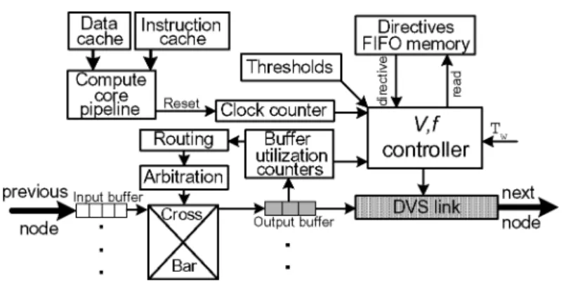
Fig. 4. Conceptual hardware design of a network router with software-directed dynamic voltage scalable links (one link shown). Note that the buffer utilization counters are connected to the routing decision circuitry only in the case of adaptive routing; this connection does not apply to routers with deterministic routing (see Section 5.2).
Rawcc compiler [Lee et al. 1998] explicitly manages all communication through the interconnect statically at compile-time, providing cycle-by-cycle message flow scheduling and timing information that can be used by LUNA. Sequencing is exact, but as a result of dynamic events there are some disturbances in run-time flows, with a 5% probability of occurrence [Lee et al. 1998]. An advantage of our methodology, as we show in Section 6.6, is that message flow-timing information does not have to be exact and can tolerate fairly large disturbances. Where static compilation is unable to analyze message flows to estimate link utilization, one can profile applications to obtain timing estimates. Saputra et al. [2002] and Xie et al. [2003], and Hu and Marculescu [2004] used this profiling approach in uniprocessors and embedded systems, respectively.
In phase 2, LUNA’s link utilization estimates are normalized to the link bandwidths, and by considering the multi-level discrete DVS model of Section 3, DVS instructions are generated for each link individually using the proposed DVS software directives algorithm of Section 4.2.
A detailed conceptual design of a software-directed router with DVS links is depicted in Fig. 4. As described in Section 4.2, the software directives are generated based upon LUNA’s sampling intervals ofTwcycles, where theseTw -based intervals form the execution time stamps and thus set the periodicity at which the directives are to be executed at network run-time. During the online phase, therefore, these directives are executed at times relevant to a hardware clock counter, i.e., at everyTw. Thus, unlike recently proposed methods [Chen et al. 2006] the software directives are not insertedin-linewith the application code, but are used in parallel with the application code; in other terms, the software directives executions are synchronized with the clock counter and not with the processor instructions. Thus, at each node, custom directives for each link are written into a dedicated FIFO memory whenever a parallelized code segment is scheduled to run on the associated node processor. The directives can be written into the FIFO memory by the operating system and can be saved/restored as a part of the context by the OS, if the application is swapped out from the system to run a second application. In this case, the OS writes
into the FIFO memory the directives applicable to the second application, while the original DVS directives are stored in the process context block of the first application. Note that as the process switches occur infrequently, the OS context switch overheads impacting the overall system are expected to be relatively small.
The node processor is responsible for resetting the clock counter when the application starts executing, while the DVS controller polls these directives from the FIFO memory periodically, paced atTwintervals, to set the voltage and frequency levels of the outgoing DVS link. Since the execution of these directives is independent of the current node’s processor, the pipeline of the processor is unaffected and no additional latencies are incurred. In short, instructions are executed by the main processor core while DVS directives are acted upon by the DVS controller, which is a state machine within the router. The FIFO memory can be of a reasonable size; for instance, ifTwis 100,000 cycles, then a 100-entry FIFO memory can hold enough directives to last for 10 million cycles of application run-time. There are two DVS directives perTw(see Section 4.2), one that reaches an intermediate (V, f) level within the currentTwand another that settles on the target (V, f) at the end of the current Tw. Hence, each entry of the software directives FIFO memory contains two (V, f) directives for each sampling period ofTwcycles: it is 8 bits wide since each directive can be represented by 4 bits, given our 10-level discrete DVS link model (described in Section 3). Memories in network routers, in the form of caches, have also been used in on-chip architectures, such as Raw, to hold instructions that direct run-time packet switching in a static network [Taylor et al. 2004]. These instructions are similarly created during static compilation.
In the third phase (Fig. 3), queueing theory principles are used to trans-late already estimated link utilizations into router output buffer utilizations. A histogram is then constructed, which shows the distribution of the entire network’s output buffer utilization by aggregating all the individual estimated output buffer utilization levels. These statistics are used to set router thresh-olds, which are stored in a threshold memory at each router. The DVS con-troller shown in Fig. 4 takes into account the output buffer utilization statistics of the buffer counter to throttle DVS instructions when short-term contention exceeding these threshold levels is detected in order to maximize network per-formance. In the case of adaptive routing, the buffer utilization statistics are also used to reach a routing decision by picking the least congested output port. Section 5 provides detailed descriptions of the proposed hardware mechanisms. We next explain each phase in detail.
4.1 Phase 1: Link Utilization Estimation
To capture spatial and temporal message flow variability in order to explore power savings, we use LUNA to estimate link utilizations across the net-work [Eisley and Peh 2004]. LUNA is a high-level netnet-work power analysis tool whose accuracy was shown to be within 5.9% of cycle-level simulators [Wang et al. 2002], with a run-time that is up to 360X faster. These attributes make LUNA suitable for compiler-directed network power analysis. LUNA abstracts
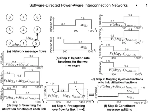
Fig. 5. A walk-through example showing the five steps of link utilization calculations using LUNA with deterministic XY routing. Time (t) is in terms of absolute router clock cycles.
network power through link utilizations, capturing the effect of contention among message flows in its estimation of utilization across time for each link in the network. Based on these estimates, we then create DVS software directives in phase 2 (Section 4.2) that leverage unused link capacity as power-saving opportunities.
There are five key steps in LUNA, explained in Fig. 5. Note that we show traffic only across router nodes 0, 1, 2, and 5 for clarity (see Fig. 5a).
Step 1. In the first step, message flows are captured asinjection rate
func-tions, with the injection rate of the message expressed as a percentage of the
injection port bandwidth over time. Figure 5b shows the injection rate functions of message flows A and B over the first 1,000 clock cycles.
Step 2. During this step, routing maps the injection rate functions of step 1 onto links of a network topology, translating them intonormalized link
utilization functions,F(Msgj,t)i, with values between 0 (no traffic) to 1.0 (link
saturated). LUNA was modified to support both deterministic XY (or static) routing, where routing messages fully traverse the X dimension before travers-ing the Y dimension toward their destination node and adaptive routtravers-ing. Both routing functions are minimal, which means that they route progressively1
within a minimum rectangle2: given the source n
s and destination nd nodes, 1In progressive routing, every routing step leads a packet one hop closer to its destination. 2A minimum rectangle applies to 2D tori, where the topology wraps at the edges causing anyn
s-nd
combination to produce four rectangles that entirely cover the topology. The minimum rectangle is the rectangle that possesses the smallest area. In meshes, wraparound links are absent and, as a result, the only rectangle formed byns-nd is also the minimum rectangle.
four rectangles contain ns and nd as their diagonally opposite vertices. The minimum rectangle is the one with the minimum diagonal distance betweenns andnd. Since both functions route progressively within a minimum rectangle they both exhibit the same hop count, q, for every packet routed along every possible ns → nd path3 between routersns andnd. In deterministic routing, this route is predetermined (exhausting the horizontal and then the vertical dimension, i.e., XY) while in adaptive routing, this route can take any staircase form, where horizontal and vertical packet traversals may alternate, each time bringing the packet a hop closer to its destination.
In this example, we demonstrate XY deterministic routing, while Sec-tion 4.1.1 explains how step 2 is modified for adaptive routing. Only step 2 is different for the two routing protocols as message routing determines mes-sage injection rate mapping, with steps 1 and 3–5 remaining identical. LUNA concurrently considers (1) the packet size in terms of flits and (2) the source-destination router coordinates of each packet (see phase 1, Fig. 3). Packet types, whether data, control, or acknowledgment, and packet contents are ignored since only the “volume” of traffic in terms of flits is required by LUNA. Figure 5c shows how message flows traverse links 0→1, 1→2, and 2→5 for the same time duration of 1,000 clock cycles. F(MsgA,t)Path(0→1) and F(MsgA,t)Path(1→2)
correspond to the normalized link utilization functions for message A over links 0→1 and 1→2, respectively. Similar notations apply for message B, as shown in Fig. 5c.
Step 3. Next, link utilization functions aresuperimposed andsummed, re-flecting the sharing of links among multiple message flows. In our example, functions F(MsgA,t)Path(1→2) andF(MsgB,t)Path(1→2) are added during 0≤t ≤
1,000 to produce F(MsgA+MsgB,t)Path(1→2). Figure 5d shows that this
sum-mation actually detects traffic contention or overflow over link 1→2 between cycles 0–300 and 600–1,000 since the normalized utilization rate of 1 is exceeded (100% link bandwidth capacity).
Step 4. To account for link contention, LUNApropagatesthis overflow area as depicted in Fig. 5e. Intuitively, this overflow area corresponds to the num-ber of bits that need to be transported later as they currently exceed the link capacity (bandwidth).
Step 5. Finally, the link utilization functions aresplitback intoconstituent
message flows, reflecting how individual messages are affected by the con-tention. Fair arbitration is assumed in splitting the link utilization among the message flows, as shown in Fig. 5f.
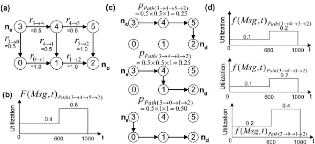
4.1.1 Adaptive Routing: Modification of LUNA’s Step 2. Adaptive routing routes progressively within a minimum rectangle, Min Rectangle(ns,nd), in a staircase manner; any possible path, Path(ns → nd), within this rectangle between source-destination nodesnsandnd can be traversed. Both static and adaptive routing exhibit the same minimal hop countqbetweennsandnd. The number of different paths that can be formed between anyns→nd router pair 3The terms “route” and “path” are used interchangeably in the paper, as well as the terms “router”
Fig. 6. Example showing a single messageM s gbeing routed from source nodens = 3 to
des-tination nodend = 2: (a) rj→j+1 next hop traversal probabilities for each link in the
mini-mum rectangle formed byMin Rectangle(ns,nd) for adaptive routing; (b) F(Msg,t) mapped
in-jection rate function for deterministic XY routing with routing pathPath(3→4→5→2); (c)
pPath(ns→nd){0,1,2}path probabilities for every link lying in the minimum rectangle (N = 3); and
(d) f(Msg,t)Path(ns→nd){0,1,2} subset link utilization functions for each routing path for adaptive routing. Time (t) is in terms of absolute router clock cycles.
is equal to the number of progressive direction combinations betweenns and
nd. These combinations cover all links in the rectangle formed betweennsand
nd. In general, if the Manhattan distance betweennsandnd consists ofqlink traversals andkN, kS,kE, kW where q = kN +kS +kE +kW are the number of traversals in the north, south, east, and west directions, respectively, then the number of different paths within Min Rectangle(ns,nd) is qCkN,kS,kE,kW =
q!
kN!kS!kE!kW!. However since we account for progressive adaptive routing within a
minimum rectangle, then only two distinguishable and progressive directions are considered and, hence,qCka,kb =
q!
ka!kb! where adesignates either the east
or west direction and b designates either the north or south direction, i.e.,
a= {E,W}andb= {N,S}. The number of paths betweenns→ nd is denoted here asN =qCka,kb. For instance, referring to Fig. 6a, the total number of paths
betweenns→nd (nodes 3 and 2) isN =3 (qCka=E,kb=N = (11!+·2!2)! =3). These three
individual paths are shown in Fig. 6c.
Only step 2, the mapping of the injection rate functions onto link utilization functions in LUNA’s five-step chain differs between deterministic and adaptive routing. Once the injection rate functions are calculated, based on the choice of routing, LUNA continues with identical calculations for the two routing cases from step 3–5 in summing and propagating the injection rate functions. Step 2 depends on the routing protocol as routing affects the path that each mes-sage takes withinMin Rectangle(ns,nd) and, therefore, the mapping of its route onto the network. For instance, Figure 6a, b show a single message,Msg, in-jected at router 3 and destined for router 2, where, in deterministic routing, this message takes the routePath(3 → 4 → 5 → 2), captured by the single link utilization function F(Msg,t)Path(3→4→5→2). With adaptive routing there
are multiple paths withinMin Rectangle(ns,nd) with each such path potentially carrying a portion of the aggregate message Msg. The superimposition of all these paths spans all links in the minimum rectangle. Thus, in adaptive rout-ingF(Msg,t)M in Rectangl e(ns,nd)is split into multiplelink utilization subfunctions f(Msg,t)Path(ns→nd)i, with each such subfunction representing a particular route Path(ns → nd)i. For each of the N distinct routing paths in a minimum rect-angle formed between ns and nd there is a corresponding and unique injec-tion rate subfuncinjec-tion f(Msg,t)Path(ns→nd)i.F(Msg,t)Min Rectangle(ns,nd)is the
sum-mation (superset) of all injection rate subfunctions for messageMsgbetween routersnsandnd, i.e.,F(Msg,t)Min Rectangle(ns,nd)=
i f(Msg,t)Path(ns→nd)i. The
injection rate subfunctions, f(Msg,t)0, f(Msg,t)1,. . ., f(Msg,t)[N−1], satisfy
the following condition for every message (each numbered subscript here de-notes a distinct path in the minimum rectangle; path notations are omitted for brevity):
F(Msg,t)= f(Msg,t)0+ f(Msg,t)1+ · · · + f(Msg,t)[N−1] (3)
Figure 6d shows how F(Msg,t)Min Rectangle(ns,nd) from Fig. 6b is split into f(Msg,t)Path(ns→nd)i wherei= {0, 1, 2}, with each such subfunction
represent-ing a distinct path between nodes ns = 3 and nd = 2. During network run-time, adaptive routing is ultimately carried out on a per-node basis, where the least congested progressive next-hop route is taken to balance network traffic among the various routing paths in hopes of achieving higher performance. Since each possible path cannot be known a priori, we emulate adaptive rout-ing by assignrout-ingnext hop traversal probabilities rj→j+1at each connecting link
that lies inMin Rectangle(ns,nd). Figure 6a shows theserj→j+1assignments. rj→j+1 lies within{0.5, 1} as we assume progressive routing, so there are at
most two possible next-hop routers for 2D topologies4 emanating from a
cur-rent router with each such next-hop router having a probabilityrj→j+1=50% of
being reached. Routers that lie at the two minimum rectangle perimeter edges touching nd carry arj→j+1 = 1 since there is only one next-hop router to be
reached.
Since each path does not carry the same distribution of rj→j+1
val-ues, this means that each possible Path(ns→nd)i does not carry the same probability of being traversed. This needs to be reflected upon the in-jection rate subfunctions f(Msg,t)Path(ns→nd)i. We define the set consisting
of pPath(ns→nd)i as the path probabilities, i.e., the probability of each
pos-sible path being traversed by a message stream between nodes ns and
nd, one for each f(Msg,t)Path(ns→nd)i. Each pPath(ns→nd)i represents the
ra-tio of traffic carried by the corresponding f(Msg,t)i, and has a value equal to the product of all the rj→j+1 of those links that lie on its path.
In other words ∀ni j ∈Path(ns→nd)i ∃rs→s+1,rs+1→s+2,. . .,rd−1→d, where
pPath(ns→nd)i =
d−1
s=0rs→s+1. For instance, the uppermost graph of Fig. 6c shows
that pPath(3→4→5→2) =r3→4×r4→5×r5→2 =0.5× 0.5×1.0 =0.25. This means
that f(Msg,t)Path(3→4→5→2) will have a probability of 0.25 of being traversed.
When the network is relatively large, this may increase LUNA’s computational time. For instance in an 8×8 mesh topology, when a corner router sends a mes-sage stream to the opposite diagonal corner (though because of parallel compiler optimizations targeting code spatial locality such probability of occurrence is very small) of the topology this can result inN = (77!7!+7)! =3432 different paths. This is impractical; to reduce the number of calculations, we select a subset of such paths. This can result in overestimation or underestimation of some
f(Msg,t)Path(ns→nd)i. However, this impact is small as Manhattan distances are
usually short and produce a smallN. Thus, the number of f(Msg,t)Path(ns→nd)i
is relatively small. Typically we choose 5≤M ≤10, whereM ≤NandMis the subset of paths out of the total number of possible pathsN. The set ofM paths chosen consists of the paths at the outer perimeter of the minimum rectangle, which have the largest path probabilities, pPath(ns→nd)i, the diagonal across the
rectangle connecting the two routers, and equally spaced paths between each side of this diagonal and the facing rectangle perimeter. The pi probabilities (we drop the path subscript from pPath(ns→nd)i and f(Msg,t)Path(ns→nd)i for
clar-ity) need to be normalized over the M paths to determine the ratio of traffic each f(Msg,t)i now takes. Since
N−1
i=0 pi =1, we let 0 <W =
M−1
i=0 pi ≤1, define a weighing factor for all f(Msg,t)i:
F(Msg,t)= p0 W f(Msg,t)0+ p1 W f(Msg,t)1+ · · · + p[M−1] W f(Msg,t)[M−1] (4)
This correctly estimates the relative proportion of traffic captured by each
f(Msg,t)Path(ns→nd)i consistently as
N−1 i=0 pPath(ns→nd)i = M−1 i=0 pPath(ns→nd)i W =1, in full agreement with the original Eq. (3). Note that the calculation of all in-jection rate functions under adaptive routing offers a conjecture of how traffic will be routed during network run-time. It is obviously impossible to predict the exact paths every message stream will take beforehand during static link utilization estimations. As routing decisions occur on-the-fly there are possible mismatches in routing between predicted paths and actual paths taken. At each hop, the routing decision chooses the least congested output link (out of the two that conform to progressive routing) based on the run-time measurement of output buffer utilizations, as will be described in Section 5.2. Though the above routing mismatches can occur, the online hardware mechanism of Section 5 helps adapt to these inconsistencies and maintain high network power-performance. Results in Section 6 show the superiority of adaptive versus static routing.
Fig. 7. Example of software-directives generation.
4.2 Phase 2: Software-Directives Extraction
Estimated link utilizations from phase 1 are used as inputs in phase 2 to gener-ate DVS software directives for each network link individually. Though phase 2 is carried out independently for each link, the link utilization estimates from phase 1 are based on global information of the message flows across an en-tire application, unlike previous limited-scope hardware methods [Shang et al. 2002; Soteriou and Peh 2004] that only used local information.
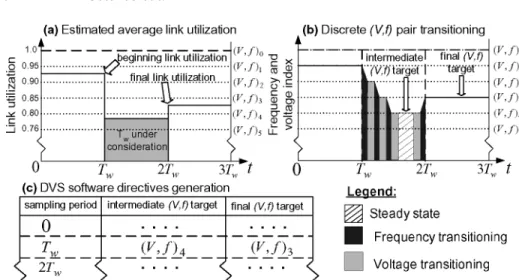
Figure 7 sketches an overview of phase 2. Intuitively, the process of gener-ating software directives works as follows: given the average link utilizations generated by LUNA in phase 1 over window intervalsTw, the method first maps these utilization levels to the closest upper discrete link voltage/frequency lev-els that can support the required bandwidth (Fig. 7a). Then, at each sampling window, starting from the voltage/frequency setting at the beginning of the sam-pling window, the algorithm lowers voltage/frequency as long as it can return to the voltage/frequency setting required at the start of the next sampling win-dow. Here, voltage/frequency transition delays come from our DVS link model (Fig. 7b). We term this lowest voltage/frequency level the intermediate (V, f) target and the voltage/frequency setting just before the start of the next win-dow as the final (V, f) target. Finally, these two directives are entered for each
Tw to create a Tw-based list of DVS software directives that are executed at run-time (Fig. 7c).
In exploring opportunities for (V, f) link reduction, our methodology works by exploiting excess link resources that reside on two axes: time and remaining unutilized link capacity on the horizontal and vertical axes, respectively (see Fig. 7a). When a link’s operating frequency is reduced, the time needed by a flit to cross that link is proportionally stretched over the horizontal axis. As our Tw-based approach is designed to satisfy the condition of prohibiting pro-gram execution spilling over the subsequentTwsegment, this link now has to transport the same volume of traffic (number of flits) at a slower pace within
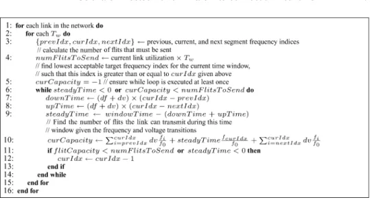
Fig. 8. Software directives generating algorithm.
the currentTwsegment. This translates to an increase in the link’s bandwidth utilization (or a decrease in the remaining link transport capacity) seen on the vertical axis within thisTw segment. The methodology recurses over con-secutive (V, f) steps to determine the specific (V, f) link level, which is just enough to satisfy the above condition, at which point a DVS directive reflecting the calculated (V, f) target level for the currentTwis generated.
Mathematically, each link utilization profile is modeled as a discrete-time function,U[Twn], wheren = 0, 1, 2,. . .,N andTw is the sampling period, or window size. As Fig. 7a shows,U[t] is a step function and is continuous on the interval [Twn,Tw(n+1)] such thatU[t]=U[Twn] fort ∈[Twn,Tw(n+1)]. Its amplitude is the average measured link bandwidth requirement, normalized so that 0 indicates zero utilization and 1 maximum capacity. The amplitude of eachU[Twn] is matched to the next higher discrete frequency fk, wherek is the frequency index ranging from 0 to 9. f0denotes full link frequency (1 GHz)
and f9the smallest available frequency (0.6 GHz).
To create (V, f) pair directives, we apply the algorithm of Fig. 8 to each network link individually to extract the intermediate and final target DVS instructions for everyTw. This is depicted in Fig. 7b and c. Though individual directives are created for eachTw, the calculations carried out in the algorithm need to consider the beginning (end of Tw(i−1)) and the end (beginning of
Tw(i+1)) link utilization levels ofTw(i), betweent = Tw andt = 2Tw, in our example. Because the calculation at a current window depends on that from the previous window, directives are created in order with respect to time.
4.2.1 Algorithm Details. The algorithm begins by translating the ampli-tude of each link utilization function Uj[Twi] for each time segment i into the smallest index k such that fk
f0 ≥ Uj[Twi]. This k is termed curIdx.
Simi-larly,prevIdx (beginning ofTw) andnextIdx(end of Tw) forU[Tw(i−1)] and
the two ends of Tw. The number of flits that will traverse a link j is the prod-uct of the current utilization level (flits/cycle) and window size (cycle count),
numFlitsToSendj = Tw ×Uj[Twi]. Figure 7a depicts numFlitsToSendj as
the shaded area between t = Tw and t = 2Tw. All these flits captured by
numFlitsToSendj must be able to traverse the link within this same time
du-ration, that is,Tw, with our calculated lower-frequency (V, f) targets.
To create DVS directives, the algorithm tracks the number of discrete (V, f) step–downs and step–ups relative to the starting and ending link utilizations of the current Tw sampling window. As an example, consider the timet =Tw to t =2Tw of Fig. 7b, where the frequency and voltage are reduced by three steps from (V, f)1 to the intermediate target of (V, f)4, and then they are
increased by one step to a final target of (V, f)3, prior to 2Tw. Specifically,
given prevIdx, curIdx, nextId, the step-down count from the beginning of a window ismax(curIdx-prevIdx, 0); the step-up count to the end of the segment
ismax(curIdx-nextIdx, 0).
To determine the final number of (V, f) step-ups/-downs within the current
Twthe algorithm begins at fcurIdxdiscrete frequency level, which can accommo-dateU[Tw], that is fcurIdxf
0 ≥U[Tw], and keeps recursing, with each recursion
replacing CurIndx withCurIndx −1 (i.e., next higher discrete-level link fre-quency), until both: (1) there is just enough time for the calculated number of (V, f) hoppings (i.e., the horizontal component is satisfied), and (2) the utilized link bandwidth can fit into the link’s maximum capacity of 1.0 (i.e., the vertical component is satisfied), andnumFlitsToSendcan be sent withinTw. The hori-zontal component is measured viasteadyTimeand the vertical viaflitCapacity.
steadyTimeis directly affected bydvanddf, the voltage and frequency
transi-tion delays, with flits unable to traverse a link duringdf(see Section 3). These are in terms of nominal router cycles with respect to f0=1 GHz, and, the time
to step down isdownTime=numStepsDown×(dv+df). Similarly the time to step-up isupTime=numStepsUp×(dv+df). The horizontal component is mea-sured via steadyTime=Tw−(downTime+upTime) and it is the time spent at the intermediate target frequency and voltage for the currentTw.
The used link capacityflitCapacityis determined by the cumulative effects of up and down (V, f) link transitions. With each (V, f) step, the link’s through-put changes directly with frequency and this effect is taken into account to determine whether flitCapacity ≥ numFlitsToSendis satisfied within Tw. At each recursive step, the algorithm calculatesflitCapacityunder the given (V, f) transitions by multiplying each frequency that the link operates at during the current segment by the number of cycles the link spends at that frequency, and summing these numbers. For our example, Fig. 7b depicts this frequency–time product as the diagonally striped area, entitled “steady state.”
The intermediate target index decrements by 1, equivalently reducing the number of step-ups/-downs in the current segment, until steadyTime≥0 and
flitCapacity≥numFlitsToSend. Following our example, Fig. 7b shows that in
or-der to reach the intermediate (V, f) target, there must be three step-down hops from (V, f)1to (V, f)4and one step-up to meet the final target of (V, f)3, after
which the availablesteadyTimeis exhausted and no more (V, f) transitions can occur. Continuing with our example of Fig. 7c, once these two voltage-frequency
Fig. 9. Wormhole router microarchitecture, depicting the physical parameters of an M/D/1 queue-ing system.
targets are calculated, software directives representing these intermediate and final (V, f)klevels are created. The algorithm then recurses over the remaining
Tw segments to create further two (V, f)k instructions for each Tw, spanning the entire application duration and all network links.
4.3 Phase 3: Output Buffer Utilization Estimation
In this phase, we make use of queueing theory principles to translate the es-timated link utilizations of phase 1 and the target link operating frequencies of phase 2 into output buffer utilization histograms. The goal here is to derive statistics to set application-specific thresholds, which guide our online DVS mechanism of Section 5.
We model each output buffer as an M/D/1 queue and estimate the utilization of each such buffer and for each sampling periodTw. Under standard queueing notation, this refers to a queue that has a Poisson flit arrival rate with average valueλ, a deterministic flit service rate of μ, and a single server (link). The service rate is considered to be deterministic since phases 1 and 2 provide information concerning the average link utilizations and operating frequencies over the entire application span. Figure 9 depicts the microarchitecture of a wormhole router with an output link connecting sender (upstream) and receiver (downstream) routers. λ is the rate of traffic on the downstream side of the crossbar. The router operating frequency fr is constant (1 GHz) with fr ≥ fl, where fl is the link frequency and is variable over 10 discrete (V, f) levels, as described in Section 3. The following equation is used to determine the average number of occupied buffers (equivalently customers in a queue) for our M/D/1 queueing system [Kleinrock 1975]
N = 2ρ−ρ
2
2(1−ρ) (5)
whereρ= λμ. This system assumes a constant service rate, however, with a DVS link the service rate varies since the software directives can set any of (V, fl)0→9
level pairs with eachTw. To account for this, we parameterizeμi,j = ffi,0j, where
fi,j is the intermediate target frequency value for link j and time Twi, and
Similarlyρi,j =μλii,,jj. Equation (5) becomes
Ni,j =
2ρi,j −ρi2,j 2(1−ρi,j)
(6) In this model, we assume that the output and input buffers have enough capac-ity to prevent overflows and we use LUNA’s estimation of link utilization (per
Tw) as the value ofλi,j. Under wormhole credit-based flow control (see Section 6.1), a flit that has permission to traverse the crossbar must have reserved a position at the output buffer of the current router and a position at the input buffer of the downstream router.
We calculate the average network buffer utilizationBUby averaging allNi,j, normalized with respect to the buffer size, over all combinations of network links and sampling periods. Specifically
BU = 1 |L| i∈L 1 |T| j∈T Ni,j |B| (7)
whereLandTare the set of links in the network and set of all sampling periods under consideration, respectively, with|L|and|T|denoting the cardinality of these sets.|B|is the buffer size in terms of flits. Next, Section 5 will describe how
BU determines thresholds that help our online DVS mechanism tune (V, f) pair transitions to maximize network performance.
5. ONLINE DVS HARDWARE MECHANISM
In this section, we describe our online DVS mechanism and its interaction with DVS software directives. The online DVS mechanism has a dual func-tion: (1) it reacts to run-time variabilities in the traffic profile, which can arise as a result of averaging effects or inaccuracies of LUNA and/or compiler-time scheduling/profiling inconsistencies (Section 5.1), and, under the adaptive rout-ing protocol, (2) it orchestrates next-hop routrout-ing decisions by choosrout-ing the least congested progressive output port (based upon online output buffer utilization measurements) at every network router (Section 5.2).
5.1 Output Buffer Thresholds
To detect online traffic variability, we compare LUNA’s statically estimated link utilization levels to the network utilization at run-time. If the latter is greater than the former, DVS directives are throttled to reduce network contention. To direct this online mechanism, we make use of statistics collected via hardware counters.
An obvious way of gathering run-time statistics is tracking link utilizations directly in hardware. However, with practical flow control methods, link utiliza-tion only tracks resource utilizautiliza-tion well at low- to mid-network traffic levels. When the network is congested, or when the link’s (V, f) level is currently set below the required bandwidth, traffic tends to get buffered in input and output buffers and link utilization leans to zero, making it an unsuitable metric [Shang et al. 2002; Soteriou and Peh 2004]. Per-port output buffer utilization, which is
buffer occupancy over the pastMrouter cycles, measured at sampling timenfor each output port at a router.BU pout[n] is calculated at every router clock cycle. In our experiments, we set M = 300 cycles for two reasons: to detect recent network contention levels and to keep the hardware compact. It is critical to keep in mind the hardware overhead involved in gathering statistics. All of our proposed statistics only require simple hardware counters.5
We use LUNA’s average network buffer utilization estimation BU from
Section 4.3 to set thresholds. Our online DVS mechanism compares these thresholds againstBU pout[n] when optimizing the execution of software direc-tives to maintain high network performance. When localized link congestion is detected, DVS (V, f) transitioning is backed off or postponed by the mechanism. Unlike previous limited-scope methodologies [Shang et al. 2002; Soteriou and Peh 2004], thresholds are not set based upon some empirical value, but are cus-tomized according to the application characteristics. Using LUNA’s statistics from Section 4.3, in particular, the average number of occupied output buffers
Ni,j
|B| for every sampling period Twi for all links j, we are able to draw a his-togram of the network’s output buffer utilization profile. In this hishis-togram the x-axis shows the normalized output buffer occupancy and the y-axis shows the number of occurrences. The aggregate sum of all occurrence values along the y-axis equals the product of the number of all sampling periods |T| and the total number of network links|L|. The derived output buffer utilization profile, though application-dependent, approximates a Gaussianlike distribution with most applications. Using this histogram we can estimate the standard devia-tionσBU, for which we base our thresholds to capture the outlier cases of higher buffer utilizations when network contention is likely to occur. Actual run-time utilization measurements of Fig. 10 show histograms of the four output buffers at a randomly chosen router in the 5×5 TRIPS CMP architecture. Though, in this example, some of the histograms skew to the left, the purpose ofσBU is to capture the outlier cases (closer to BUP out[n]1) of higher buffer utilizations at which network congestion is most likely to occur. To capture these outlier points, we make use of the following three threshold levels; an explanation of their use follows
ThBUhigher = BU+ασBU (9)
5The power consumed by counters is ignored, as similar hardware has been shown to consume
Fig. 10. Histograms showing output buffer utilization profiles of the four output buffer ports at a randomly chosen router in a 5×5 TRIPS mesh inter-ALU interconnection network running the bzip2benchmark. Each buffer utilization occurrence is measured across 500 cycles of simulation time with the architecture configuration parameters shown in Table II
ThBUhigh = BU+βσBU (10)
ThBUlow = γBU (11)
where the above constants are set as follows:
0< β < α, γ <1 (12) The various thresholds act as follows: when BU pout[n] > ThBUhi g h and BU pout[n]<ThBUhigher, the algorithm postpones software directives for a retry
period tretry. We set tretry = 240 cycles in our experiments, 2×(d v+d f), so as to facilitate a near-future retry test for DVS directives execution. When
BU pout[n]>T hBUhigher, the algorithm ignores software directives, and the link
transitions to a higher voltage/frequency. If any of the above cases occur and iftretryhas elapsed, the link transitions to a lower (V, f) pair approaching the intermediate (V, f) target only ifBU pout[n]<ThBUlow.
Essentially DVS software directives acts as recommendationsfor setting (V, f) target pairs for everyTw, while the online mechanism acts as the final
de-ciderof setting these levels according to the various conditions just described.
The directives present a lower bound for (V, f) targets for power optimiza-tion, while the online mechanism allows (V, f) pairs to float above this lower bound, conservatively delaying/ignoring power-savings opportunities in favor of performance.
Figure 11 exhibits the behavior of a software-directed network. It shows the (V, f) transitions for two consecutiveTw windows. In the upper part, the link transitions from (V, f)1 to reach the intermediate target (V, f)4. At (V, f)3, BU pout[n] > ThBUhigh postponing a further down-ramp for a time duration of tretry. When this time has elapsed, it tests for BU pout[n] < T hBUlow, which is
not satisfied, postponing (V, f)3→4 for another tretry. At the nexttretry expira-tion, BU pout[n] satisfies the threshold test and so (V, f)3→4 transitioning is
performed. Also note that enoughsteadyTimeis present with respect to time
t = Tw for performing this transition. At tramp-up the link starts up-ramping (V, f)4→3to meet the final (V, f)3target at the end oft=Tw.
In the lower part of Fig. 11, the link starts from (V, f)3to try to reach the final
(equals to the intermediate) (V, f)5target. From the startBU pout[n]>ThBUhigh
Fig. 11. Online DVS (V, f) transitioning example.
tretry has elapsed, BU pout[n] is consulted, BU pout[n] > ThBUhigher and the link
back-offs up-ramping (V, f)3→2. Atretryis elapsed where BU pout[n]>T hBUlow,
setting anothertretryat which BU pout[n]< T hBUlow, and the link down-ramps
(V, f)2→3, and subsequently, (V, f)3→4. The link does not reach the target
(V, f)5 level since it has exhausted steadyTime(tremain < d v+d f) with re-spect tot=2Tw. The mechanism will then try to reach the (V, f) intermediate and final target levels within the next Tw (recursive behavior). This example demonstrates the adaptive nature of the online mechanism. It tunes the links to maintain performance over short-term changes in network contention and, at the same time, it attempts to meet the target (V, f) levels to lower power consumption.
5.2 Adaptive Routing Using Online Buffer Utilization Measurements
The output buffer utilization levels (BU pout[n] of Eq. 8) measured at every router, are used dually under adaptive routing: (1) to throttle DVS directives when high contention levels are detected, as in the case of static routing, and (2) to orchestrate per-hop routing decisions. This section provides details for the latter case.
As described in Section 4.1.1, software directives statically generated for run-time adaptive routing need to synchronize with on-the-fly per-hop adaptive routing decisions. With progressive adaptive routing, there are either one or two output link alternatives to be considered at each router. The link with the lower output buffer utilization is chosen for a next-hop packet traversal. For instance, at the timenof reaching a routing decision at a router, if the east port’s output
Table II. Configurations of Simulated Architectures
Architecture Network Pipeline Input/output Packet size size length buffer size (#flits) (flit count)
Raw 4×4 5/1a 5/5 1
TRIPS 5×5 5 10/10 3
Alpha 21364 8×8 13 128/128 16 and 80
aIn Raw, the static router is a five-stage pipeline. The router decodes switching instruc-tions to set up a path in advance (see Section 6.2). Once the path is established, every flit encounters a unit delay in the sender and receiver router ALUs in ALU to ALU communication, plus the link delay.
buffer utilization is greater than the south port’s buffer utilization (BU peast[n]>
BU psouth[n]) and assuming that both routing directions are progressive (see Section 4.1.1), then the south link will be chosen as it exhibits lesser contention. This process will be repeated at the next downstream router until the packet reaches its destination and is finally ejected from the network, i.e., routing decisions are carried out on a per-hop basis.
6. EXPERIMENTAL SETUP AND RESULTS 6.1 Simulator Setup
To evaluate power-latency tradeoffs of our approach, we simulated paral-lelized code running on three existing network architectures with software-directed DVS links. These architectures are the Raw [Taylor et al. 2004] and TRIPS [Sankaralingam et al. 2003] single-chip multiprocessors (CMPs), and an Alpha 21364-based multi-chip server [Mukherjee et al. 2002]. Details of these architectures are provided in subsequent subsections. Our simulator models an event-driven wormhole switching network with credit-based flow control at the flit level [Duato 1997], extending upon PoPNet [Shang 2002], a publicly available simulator. The simulator supports deterministic and adaptive routing protocols, described in Sections 4.1 and 4.1.1.
The simulator supports k-ary 2-mesh topologies with 1 GHz multi-stage pipelined router cores, each with two virtual channels. Packets are composed of 32-bit flits with each flit transported in 1 link cycle over links of 32 Gbps bandwidth. Each router consists of eight unidirectional channels (four incom-ing and four outgoincom-ing). Table II provides a summary of our simulated network architectures.
In all our experiments, we setThBUhigher =BU+ 5 4σBU,ThBUhigh =BU+ 3 4σBU andThBUlow = 3
4BU.tretryis set to 240 cycles, which is 2×(d v+d f) andTw =
20, 000 cycles. Each simulation is run for the entire trace length measuring up to 10 s of millions of cycles. The metrics considered are latency and power consumption. Latency spans the injection of the head flit of a packet until its tail flit is ejected from the destination router. Link power savings is the ratio of the aggregate power consumption across all links in the network with DVS, divided by the power consumption of all links operating at full frequency (no DVS). The link power savings shown in the subsequent results translate to overall system power savings of approximately 10 to 15% in chip-to-chip parallel systems and to