services produced in a country. GDP is part of the national income and product accounts(or national accounts), which are a body of statistics that enable pol-icymakers to determine whether the economy is contracting or ex-panding and whether a severe recession or inflation threatens. When economists want to determine the level of economic
de-velopment of a country, they look at its GDP per capita. While the GDP and the rest of the national accounts may seem to be arcane concepts, they are truly among the great inventions of the twentieth century. Much as a satellite in space can survey the weather across an entire continent, so can the GDP give an overall pic-ture of the state of the economy. In this chapter, we explain how economists measure GDP and
other major macroeconomic concepts.
GROSS DOMESTIC PRODUCT:
THE YARDSTICK OF AN
ECONOMY’S PERFORMANCE
What is the gross domestic product? GDP isthe name we give to the total market value of the final goods and services produced within a nation during a given year. It is the figure you get when you apply the measuring rod of money to the diverse goods and services—from apples to zithers—that a country produces with its land, labor, and capital resources. GDP equals the total production of consump-tion and investment goods, government purchases, and net exports to other lands. The gross domestic product (GDP) is the most comprehensive measure of a nation’s to-tal output of goods and services. It is the sum of the dollar values of consumption (C), gross investment (I), government purchases of goods and services (G), and net exports (X) produced within a nation during a given year.
In symbols:
GDPCIGX
GDP is used for many purposes, but the most important one is to measure the overall performance of an economy. If you were to ask an economic historian what happened during the Great Depression, the best short answer would be:
Between 1929 and 1933, GDP fell from $104 billion to $56 billion. This sharp decline in the dollar value of goods and services produced by the American economy caused high unemployment, hardship, a steep stock market decline, bankruptcies, bank failures, riots, and political turmoil.
Measuring Economic
Activity
When you can measure what you are speaking about, and express it
in numbers, you know something about it; when you cannot measure it, when you cannot
express it in numbers, your knowledge is of a meager and unsatisfactory kind; it may be the
beginning of knowledge, but you have scarc e l y, in your thoughts, advanced to the stage of science.
Lord Kelvin
88
5
C H A P T E R
Similarly, if you were to ask what was unusual about the 1990s, a macroeconomist might reply:
The 1990s were the longest economic expansion in the nation’s history. From 1992 to 2000, real GDP grew steadily, increasing by 37 percent with falling unemployment, stable inflation, and rising stock-market prices.
We now discuss the elements of the national in-come and product accounts. We start by showing dif-ferent ways of measuring GDP and distinguishing real from nominal GDP. We then analyze the major components of GDP. We conclude with a discussion
of the measurement of the general price level and the rate of inflation.
Two Measures of National Product:
Goods Flow and Earnings Flow
How do economists actually measure GDP? One of the major surprises is that we can measure GDP in two entirely independent ways. As Figure 5-1 shows, GDP can be measured either as a flow of products or as a sum of earnings.
To demonstrate the different ways of measuring GDP, we begin by considering an oversimplified
GROSS DOMESTIC PRODUCT: THE YARDSTICK OF AN ECONOMY’S PERFORMANCE
89
Circular Flow of Macroeconomic Activity
$
Consumption purchases
(a)
Final goods and services (bread, computers, haircuts, etc.)
(b) Productive services
(labor, land, etc.)
Wages, rents, profit, etc. $ Purchasers (households, governments, . . .) Producers (businesses)
FIGURE 5-1. Gross Domestic Product Can Be Measured Either as (a) a Flow of Final Products or, Equivalently, as (b) a Flow of Costs
In the upper loop, purchasers buy final goods and services. The total dollar flow of their spending each year is one measure of gross domestic product. The lower loop measures the annual flow of costs of output: the earnings that businesses pay out in wages, rent, interest, dividends, and profits.
The two measures of GDP must always be identical. Note that this figure is the macro-economic counterpart of Fig. 2-1, which presented the circular flow of supply and demand.
approach and by the lower-loop earnings-flow ap-proach. Which is the better approach? The surprise is that they are exactly the same.
We can see why the product and earnings ap-proaches are identical by examining a simple bar-bershop economy. Say the barbers have no expenses other than labor. If they sell 10 haircuts at $8 each, GDP is $80. But the barbers’ earnings (in wages and profits) are also exactly $80. Hence, the GDP here is identical whether measured as flow of products ($80 of haircuts) or as cost and income ($80 of wages and profits).
In fact, the two approaches are identical because we have included “profit” in the lower loop along with other incomes. What exactly is profit? Profit is what remains from the sale of a product after you have paid the other factor costs—wages, interest, and rents. It is the residual that adjusts automatically to make the lower loop’s costs or earnings exactly match the upper loop’s value of goods.
To sum up:
GDP, or gross domestic product, can be measured in two different ways: (1) as the flow of final prod-ucts, or (2) as the total costs or earnings of inputs producing output. Because profit is a residual, both approaches will yield exactly the same total GDP.
National Accounts Derived from
Business Accounts
You might wonder where on earth economists find all the data for the national accounts. In practice, government economists draw on a wide array of sources, including surveys, income-tax returns, retail-sales statistics, and employment data.
The most important source of data is business ac-counts. An accountfor a firm or nation is a numeri-cal record of all flows (outputs, costs, etc.) during a given period. We can show the relationship between business accounts and national accounts by con-structing the accounts for an economy made up only of farms. The top half of Table 5-1 shows the results of a year’s farming operations for a single, typical farm. We put sales of final products on the left-hand side and the various costs of production on the right. The bottom half of Table 5-1 shows how to construct the GDP accounts for our simple agrarian economy in which all final products are produced on 10 mil-lion identical farms. The national accounts simply add together or aggregatethe outputs and costs of the world in which there is no government, foreign
trade, or investment. For the moment, our little economy produces only consumption goods,which are items that are purchased by households to satisfy their wants. (Important note: Our first example is oversimplified to show the basic ideas. In the realis-tic examples that follow, we will add investment, gov-ernment, and the foreign sector.)
Flow-of-Product Approach. Each year the public consumes a wide variety of final goods and services: goods such as apples, computer software, and blue jeans; services such as health care and haircuts. We include only final goods—goods ultimately bought and used by consumers. Households spend their in-comes for these consumer goods, as is shown in the upper loop of Figure 5-1. Add together all the con-sumption dollars spent on these final goods, and you will arrive at this simplified economy’s total GDP.
Thus, in our simple economy, you can easily cal-culate national income or product as the sum of the annual flow of finalgoods and services: (price of blue jeansnumber of blue jeans) plus (price of applesnumber of apples) and so forth for all other final goods. The gross domestic product is defined as the total money value of the flow of fi-nal products produced by the nation.
National accountants use market prices as weights in valuing different commodities because market prices reflect the relative economic value of diverse goods and services. That is, the relative prices of dif-ferent goods reflect how much consumers value their last (or marginal) units of consumption of these goods. Earnings or Cost Approach. The second and equiv-alent way to calculate GDP is the earnings or cost ap-proach. Go to the lower loop in Figure 5-1. Through it flow all the costs of doing business; these costs in-clude the wages paid to labor, the rents paid to land, the profits paid to capital, and so forth. But these business costs are also the earnings that households receive from firms. By measuring the annual flow of these earnings or incomes, statisticians will again ar-rive at the GDP.
Hence, a second way to calculate GDP is as the total of factor earnings (wages, interest, rents, and profits) that are the costs of producing society’s fi-nal products.
Equivalence of the Two Approaches. Now we have calculated GDP by the upper-loop flow-of-product
10 million identical farms to get the two different measures of GDP.
The Problem of “Double Counting”
We defined GDP as the total production of final goods and services. A final productis one that is pro-duced and sold for consumption or investment. GDP excludes intermediate goods—goods that are used up to produce other goods. GDP therefore includes bread but not wheat, and home computers but not computer chips.For the flow-of-product calculation of GDP, ex-cluding intermediate products poses no major plications. We simply include the bread and com-puters in GDP but avoid including the wheat and dough that went into the bread or the chips and plas-tic that went into the computers. If you look again at the upper loop in Figure 5-1, you will see that bread and computers appear in the flow of products, but you will not find any flour or computer chips.
What has happened to products like flour and computer chips? They are intermediate products and are simply cycling around inside the block marked “Producers.” If they are not bought by con-sumers, they never show up as final products in GDP.
“Value Added” in the Lower Loop. A new statistician who is being trained to make GDP measurements might be puzzled, saying:
I can see that, if you are careful, your upper-loop product approach to GDP will avoid including inter-mediate products. But aren’t you in some trouble when you use the lower-loop cost or earnings ap-proach?
After all, when we gather income statements from the accounts of firms, won’t we pick up what grain merchants pay to wheat farmers, what bakers pay to grain merchants, and what grocers pay to bak-ers? Won’t this result in double counting or even triple counting of items going through several pro-ductive stages?
GROSS DOMESTIC PRODUCT: THE YARDSTICK OF AN ECONOMY’S PERFORMANCE
91
(a) Income Statement of Typical Farm
Output in Farming Earnings
Sales of goods (corn, apples, etc.) $1,000 Costs of production:
Wages $ 800 Rents 100 Interest 25 Profit (residual) 75 ______ ______ Total $1,000 Total $1,000
(b) National Product Account (millions of dollars)
Upper-Loop Flow of Product Lower-Loop Flow of Earnings
Final output (101,000) $10,000 Costs or earnings:
Wages (10800) $ 8,000 Rents (10100) 1,000 Interest (1025) 250 Profit (1075) 750 _______ _______ GDP Total $10,000 GDP Total $10,000
TABLE 5-1. Construction of National Product Accounts from Business Accounts
Part (a) shows the income statement of a typical farm. The left side shows the value of pro-duction, while the right side shows the farm’s costs. Part (b) then adds up or aggregates the 10 million identical farms to obtain total GDP. Note that GDP from the product side exactly equals GDP from the earnings side.
(1) final sales of bread and (2) total earnings, cal-culated as the sum of all values added in all the dif-ferent stages of bread production.
Value-added approach: To avoid double count-ing, we take care to include only final goods in GDP and to exclude the intermediate goods that are used up in making the final goods. By measuring the value added at each stage, taking care to subtract expen-ditures on the intermediate goods bought from other firms, the lower-loop earnings approach prop-erly avoids all double counting and records wages, interest, rent, and profit exactly one time.
DETAILS OF THE NATIONAL
ACCOUNTS
Now that we have an overview of the national income and product accounts, we will proceed, in the rest of this chapter, on a whirlwind tour of the various sec-tors. Before we start on the journey, look at Table 5-3 to get an idea of where we are going. This table shows a summary set of accounts for both the prod-uct and the income sides. If you know the strprod-ucture These are good questions, but there is an
ingen-ious answer that resolves the problem. In making lower-loop earnings measurements, statisticians are very careful to include in GDP only a firm’s value added. Value added is the difference between a firm’s sales and its purchases of materials and serv-ices from other firms.
In other words, in calculating the GDP earnings or value added by a firm, the statistician includes all costs except for payments made to other businesses. Hence business costs in the form of wages, salaries, interest payments, and dividends are included in value added, but purchases of wheat or steel or elec-tricity are excluded from value added. Why are all the purchases from other firms excluded from value added to obtain GDP? Because those purchases will get properly counted in GDP in the values added by other firms.
Table 5-2 uses the stages of bread production to illustrate how careful adherence to the value-added approach enables us to subtract purchases of inter-mediate goods that show up in the income state-ments of farmers, millers, bakers, and grocers. The final calculation shows the desired equality between
Bread Receipts, Costs, and Value Added (cents per loaf)
(1) (2) (3)
Less:Cost of Value added
Stage of intermediate (wages, profit, etc.)
production Sales receipts products (3)(1)(2)
Wheat 23 0 23
Flour 53 23 30
Baked dough 110 53 57
Final product: bread 190___ 110___ ___80
Total 376 186 190
(sum of value added) TABLE 5-2. GDP Sums Up Value Added at Each Production Stage
To avoid double counting of intermediate products, we calculate value added at each stage of production. This involves subtracting all the costs of materials and intermediate products bought from other businesses from total sales. Note that every black intermediate-product item both appears in column (1) and is subtracted in the next stage of production in col-umn (2). (How much would we overestimate GDP if we counted all receipts, not just value added? The overestimate would be 186 cents per loaf.)
of the table and the definitions of the terms in it, you will be well on your way to understanding GDP and its family of components.
Real vs. Nominal GDP: “Deflating”
GDP by a Price Index
We define GDP as the dollar value of goods and serv-ices. In measuring the dollar value, we use the meas-uring rod of market pricesfor the different goods and services. But prices change over time, as inflation generally sends prices upward year after year. Who would want to measure things with a rubber yard-stick—one that stretches in your hands from day to day—rather than a rigid and invariant yardstick?
The problem of changing prices is one of the problems economists have to solve when they use money as their measuring rod. Clearly, we want a measure of the nation’s output and income that uses an invariant yardstick. Economists can replace the elastic yardstick with a reliable one by removing the price-increase component so as to create a real or quantity index of national output.
Here is the basic idea: We can measure the GDP for a particular year using the actual market prices of that year; this gives us the nominal GDP,or GDP at current prices. But we are usually more interested in determining what has happened to the real GDP, which is an index of the volume or quantity of goods and services produced. We measure real GDP by
mul-tiplying the quantities of goods by an invariant or fixed set of prices. Hence, nominal GDP is calculated using changing prices while real GDP is calculated using constant prices.
When we divide nominal GDP by real GDP, we obtain the GDP deflator,which serves as a measure of the overall price level. We can calculate real GDP by dividing nominal GDP by the GDP deflator.
A simple example will illustrate the general idea. Say that a country produces 1000 bushels of corn in year 1 and 1010 bushels in year 2. The price of a bushel is $1 in year 1 and $2 in year 2. We can cal-culate nominal GDP (PQ) as $11000$1000 in year 1 and $21010$2020 in year 2. Nominal GDP therefore grew by 102 percent between the two years. But the actual amount of output did not grow anywhere near that rapidly. To find real output, we need to consider what happened to prices. We use year 1 as the base year, or the year in which we meas-ure prices. We set the price index, the GDP deflator, as P11 in the first, or base, year. From the data in the previous paragraph, we see that the GDP defla-tor is P2$2/$12 in year 2. Real GDP (Q) is equal to nominal GDP (P Q) divided by the GDP de-flator (P). Hence real GDP was equal to $1000/1 $1000 in year 1 and $2020/2$1010 in year 2. Thus the growth in real GDP, which corrects for the change in prices, is 1 percent and equals the growth in the output of corn, as it should.
DETAILS OF THE NATIONAL ACCOUNTS
93
Product approach Earnings approach
Components of gross domestic product: Earnings or costs as sources of gross domestic product:
Consumption (C) Wages, salaries, and other labor income
Gross private domestic investment (I) Interest, rent, and other property income
Government purchases (G) Indirect taxes
Net exports (X) Depreciation
Profits
Equals: Gross domestic product Equals: Gross domestic product
TABLE 5-3. Overview of the National Income and Product Accounts
This table presents the major components of the two sides of the national accounts. The left side shows the components of the product approach (or upper loop); the symbols C, I,
G, and Xare often used to represent these four items of GDP. The right side shows the com-ponents of the earnings or cost approach (or lower loop). Each approach will ultimately add up to exactly the same GDP.
the prices and quantities of important goods are changing rapidly. For example, over the last two decades, computer prices have been falling very sharply while the quantity of computers produced has risen rapidly (we return to this issue in our dis-cussion of price indexes below).
When relative prices are changing sharply, using prices of a given year will give a misleading estimate of real GDP growth. To correct for this bias, statisti-cians use chain weights. Instead of keeping the rela-tive weights on each good fixed (say, by using prices for a given year, like 1990), chain weights change each year to reflect the evolving spending patterns in the economy. Today, the official U.S. government measures of GDP and GDP price index rely upon chain weights. The technical names for these con-structs are “real GDP in chained dollars” and the “chain-type price index for GDP.”1For simplicity, we A 1929–1933 comparison will illustrate the
de-flation process for an actual historical episode. Table 5-4 gives nominal GDP figures of $104 billion for 1929 and $56 billion for 1933. This represents a 46 percent drop in nominal GDP from 1929 to 1933. But the government estimates that prices on average dropped about 23 percent over this period. If we choose 1929 as our base year, with the GDP deflator of 1 in that year, this means that the 1933 price in-dex was about 0.77. So our $56 billion 1933 GDP was really worth much more than half the $104 billion GDP of 1929. Table 5-4 shows that real GDP fell to only seven-tenths of the 1929 level: in terms of 1929 prices, or dollars of 1929 purchasing power, real GDP fell to $73 billion. Hence, part of the near-halving shown by the nominal GDP was due to the rapidly declining price level, or deflation, during the Great Depression.
The black line in Figure 5-2 shows the growth of nominal GDP since 1929, expressed in the actual dol-lars and prices that were current in each historical year. Then, for comparison, the real GDP, expressed in 1996 dollars, is shown in blue. Clearly, much of the increase in nominal GDP over the last half-cen-tury is due to inflation in the price units of our money yardstick.
Table 5-4 shows the simplest way of calculating real GDP and the GDP deflator. Sometimes these cal-culations give misleading results, particularly when
(1) (2) (3)
Nominal Index number Real GDP
GDP of prices ($, billion,
(current $, (GDP deflator, 1929 prices)
Date billion) 19291) (3)( ( 1 2 ) ) 1929 104 1.00 1 1 . 0 0 4 0 104 1933 56 0.77 0 5 .7 6 7 73
TABLE 5-4.Real (or Inflation-Corrected) GDP Is Obtained by Dividing Nominal GDP by the GDP Deflator
Using the price index of column (2), we deflate column (1) to get real GDP, column (3). (Riddle: Can you show that 1929’s real GDP was $80 billion in terms of 1933 prices? Hint: With 1933 as a base of 1, 1929’s price index is 1.30.)
1
The process of chain weighting involves linking the output or price series together by multiplying the growth rates from one period to another. An example for a haircut economy will show how this works. Say that the value of the haircuts was $300 in 1998. Further suppose that the quantity of hair-cuts increased by 1 percent from 1998 to 1999 and by 2 per-cent from 1999 to 2000. Then the value of real GDP in 1998 prices would be $300 in 1998, $3001.01$303 in 1999, and $3031.02$309.06 in 2000. The same procedure would be used to construct the chain price index. With mul-tiple outputs, we simply add together the outputs of the dif-ferent components of apples, bananas, catamarans, etc.
generally refer to real GDP and the GDP deflator, whose movements track the chain indexes very closely.
To summarize:
Nominal GDP (PQ) represents the total money value of final goods and services produced in a given year, where the values are expressed in terms of the market prices of each year. Real GDP (Q) removes price changes from nominal GDP and calculates GDP in constant prices. The traditional GDP defla-tor (P) is the “price of GDP” and is defined as fol-lows: Qreal GDP n G o D m P in d a e l fl G at D o P r P P Q
To correct for rapidly changing relative prices, the U.S. national accounts use chain weights to construct real GDP and price indexes.
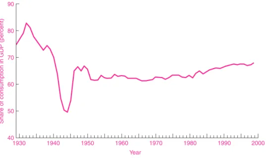
Consumption
The first important part of GDP is consumption, or “personal consumption expenditures.” Consump-tion is by far the largest component of GDP, equal-ing about two-thirds of the total in recent years. Fig-ure 5-3 shows the fraction of GDP devoted to consumption over the last six decades. Consumption expenditures are divided into three categories: durable goods such as automobiles, nondurable goods such as food, and services such as medical care. The most rapidly growing sector is services.
DETAILS OF THE NATIONAL ACCOUNTS
95
Gross domestic product
(billions of dollars per y
e ar) Real GDP (1996 prices) Nominal GDP (current prices) Year 1,000 600 100 200 400 2,000 4,000 6,000 8,000 10,000 2000 1990 1980 1970 1960 1950 1940 1930
FIGURE 5-2. Nominal GDP Grows Faster than Real GDP Because of Price Inflation The rise in nominal GDP exaggerates the rise in output. Why? Because growth in nominal GDP includes increases in prices as well as growth in output. To obtain an accurate meas-ure of real output, we must correct GDP for price changes. (Source: U.S. Department of Commerce.)
How does investment fit into the national ac-counts? If people are using part of society’s produc-tion possibilities for capital formaproduc-tion rather than for consumption, economic statisticians recognize that such outputs must be included in the upper-loop flow of GDP. Investments represent additions to the stock of durable capital goods that increase produc-tion possibilities in the future. So we must modify our original definition to read:
Gross domestic product is the sum of all final products. Along with consumption goods and serv-ices, we must also include gross investment.
Investment and Capital Formation
So far, our analysis has banished all capital. In real life, however, nations devote part of their output to production of capital—durable goods that increase future production. Increasing capital requires the sacrifice of current consumption to increase future consumption. Instead of eating more pizza now, peo-ple build new pizza ovens to make it possible to pro-duce more pizza for future consumption.In the accounts, investmentconsists of the addi-tions to the nation’s capital stock of buildings, equip-ment, software, and inventories during a year. The national accounts include mainly tangible capital (such as buildings and computers) but omit most in-tangible capital (such as research and development or educational expenses). 90 80 60 50 40 1930
Share of consumption in GDP (percent)
Year
1940 1950 1960 1970 1980 1990 2000
70
FIGURE 5-3. Share of Consumption in National Output Has Risen Recently
The share of consumption in total GDP rose during the Great Depression as investment prospects soured, then shrank sharply during World War II when the war effort displaced civilian needs. In the last two decades, consumption has grown more rapidly than total out-put as the national savings rate and government purchases have declined. (Source: U.S. Department of Commerce.)
Real investment versus financial investment
Economists define “investment” (or some-times real investment) as production of durable capital goods. In common usage, “in-vestment” often denotes using money to buy
General Motors stock or to open a savings account. For clarity, economists call this financial investment. Try not to confuse these two different uses of the word “investment.” If I take $1000 from my safe and buy some Internet stocks, this is not what macroeconomists call investment. I have simply exchanged one financial asset for another. Investment takes place when a physical capital good is produced.
Net vs. Gross Investment. Our revised definition in-cludes “gross investment” along with consumption. What does the word “gross” mean in this context? It indicates that investment includes all investment goods produced. Gross investment is not adjusted for depreciation,which measures the amount of capital that has been used up in a year. Thus gross invest-ment includes all the machines, factories, and houses built during a year—even though some were pro-duced simply to replace some old capital goods that burned down or were thrown on the scrap heap.
If you want to get a measure of the increase in society’s capital, gross investment is not a sensible measure. Because it excludes a necessary allowance for depreciation, it is too large—too gross.
An analogy to population will make clear the im-portance of considering depreciation. If you want to measure the increase in the size of the population, you cannot simply count the number of births, for this would clearly exaggerate the net change in pop-ulation. To get population growth, you must also sub-tract the number of deaths.
The same point holds for capital. To find the net increase in capital, you must start with gross invest-ment and subtract the deaths of capital in the form of depreciation, or the amount of capital used up. Thus to estimate capital formation we measure
net investment. Net investment is always births of cap-ital (gross investment) less deaths of capcap-ital (capcap-ital depreciation):
Net investment equals gross investment minus depreciation.
Government
Up to now we have talked about consumers but ig-nored the biggest buyers of all—federal, state, and local governments. Somehow GDP must take into
ac-count the billions of dollars of product a nation
col-lectivelyconsumes or invests. How do we do this? Measuring government’s contribution to na-tional output is complicated because most govern-ment services are not sold on the marketplace. Rather, government purchases both consumption-type goods (like food for the military) and invest-ment-type items (such as computers or roads). In measuring government’s contribution to GDP, we simply add all these government purchases to the flow of consumption, investment, and, as we will see later, net exports.
Hence, all the government payroll expenditures on its employees plus the costs of goods it buys from private industry (lasers, roads, and airplanes) are in-cluded in this third category of flow of products, called “government consumption expenditures and gross investment.” This category equals the contri-bution of federal, state, and local governments to GDP.
Exclusion of Transfer Payments. Does this mean that every dollar of government expenditure is included in GDP? Definitely not. GDP includes only govern-ment purchases of goods and services; it excludes spending on transfer payments.
Government transfer paymentsare government
payments to individuals that are not made in ex-change for goods or services supplied. Examples of government transfers include unemployment insur-ance, veterans’ benefits, and old-age or disability pay-ments. These payments meet important social pur-poses, but, since they are not purchases of current goods or services, they are omitted from GDP.
Thus if you receive a wage from the government because you are a teacher, your wage is a factor pay-ment and would be included in GDP. If you receive a welfare payment because you are poor, that pay-ment is not in return for a service but is a transfer payment and would be excluded from GDP.
One peculiar government transfer payment is the interest on the government debt. Interest is treated as a payment for debt incurred to pay for past wars or government programs and is not considered to be a purchase of a current good or service. Govern-ment interest payGovern-ments are considered transfers and are therefore omitted from GDP.
Finally, do not confuse the way the national ac-counts measure government spending on goods and
services (G) with the official government budget.
When the Treasury measures its expenditures, it
in-cludes expenditures on goods and services (G) plus
transfers.
Taxes. In using the flow-of-product approach to compute GDP, we need not worry about how the gov-ernment finances its spending. It does not matter whether the government pays for its goods and serv-ices by taxing, by printing money, or by borrowing. Wherever the dollars come from, the statistician computes the governmental component of GDP as the actual cost to the government of the goods and services.
of the United States. Production differs from sales in the United States in two respects. First, some of our production (Iowa wheat and Boeing aircraft) is bought by foreigners and shipped abroad, and these items constitute our exports. Second, some of what we consume (Mexican oil and Japanese cars) is pro-duced abroad and shipped to the United States, and such items are American imports.
A Numerical Example. We can use a simple farming economy to understand how the national accounts work. Suppose that Agrovia produces 100 bushels of corn and 7 bushels are imported. Of these, 87 bushels are consumed (in C), 10 go for government purchases to feed the army (as G), and 6 go into do-mestic investment as increases in inventories (I). In addition, 4 bushels are exported, so net exports (X) are 47, or minus 3.
What, then, is the composition of the GDP of Agrovia? It is the following:
GDP87 of C10 of G6 of I3 of X 100 bushels
Gross Domestic Product, Net Domestic
Product, and Gross National Product
Although GDP is the most widely used measure of national output in the United States, two other con-cepts are frequently cited: net domestic product and gross national product.Recall that GDP includes grossinvestment, which is net investment plus depreciation. A little thought But while it is fine to ignore taxes in the
flow-of-product approach, we must account for taxes in the earnings or cost approach to GDP. Consider wages, for example. Part of my wage is turned over to the government through personal income taxes. These direct taxes definitely do get included in the wage component of business expenses, and the same holds for direct taxes (personal or corporate) on interest, rent, and profit.
Or consider the sales tax and other indirect taxes that manufacturers and retailers have to pay on a loaf of bread (or on the wheat, flour, and dough stages). Suppose these indirect taxes total 10 cents per loaf, and suppose wages, profit, and other value-added items cost the bread industry 90 cents. What will the bread sell for in the product approach? For 90 cents? Surely not. The bread will sell for $1, equal to 90 cents of factor costs plus 10 cents of indirect taxes. Thus the cost approach to GDP includes both in-direct and in-direct taxes as elements of the cost of pro-ducing final output.
Net Exports
The United States is an open economy engaged in importing and exporting goods and services. The last component of GDP—and an increasingly im-portant one in recent years—is net exports,the dif-ference between exports and imports of goods and services.
How do we draw the line between our GDP and other countries’ GDPs? The U.S. GDP represents all goods and services produced within the boundaries
1. GDP from the product side is the sum of four major components: • Personal consumption expenditure on goods and services (C) • Gross private domestic investment (I)
• Government consumption expenditures and gross investment (G) • Net exports of goods and services (X), or exports minus imports
2. GDP from the cost side is the sum of the following major components:
• Wages and salaries, interest, rents, and profit (always with the careful exclusion, by the value-added technique, of double counting of intermediate goods bought from other firms)
• Indirect business taxes that show up as an expense of producing the flow of products • Depreciation
3. The product and cost measures of GDP are identical(by adherence to the rules of value-added bookkeeping and the definition of profit as a residual).
4. Net domestic product (NDP) equals GDP minus depreciation.
suggests that including depreciation is rather like in-cluding wheat as well as bread. A better measure would include only netinvestment in total output. By subtracting depreciation from GDP we obtain net do-mestic product(NDP). If NDP is a sounder measure of a nation’s output than GDP, why do national ac-countants focus on GDP? They do so because de-preciation is somewhat difficult to estimate, whereas gross investment can be estimated fairly accurately. An alternative measure of national output, widely used until recently, is gross national product(GNP). What is the difference between GNP and GDP? GNP is the total output produced with labor or capital owned
by U.S. residents, while GDP is the output produced with labor and capital located insidethe United States. For example, some of the U.S. GDP is produced in Honda plants that are owned by Japanese corpora-tions. The profits from these plants are included in U.S. GDP but not in U.S. GNP because Honda is a Japanese company. Similarly, when an American econ-omist flies to Japan to give a paid lecture on baseball economics, payment for that lecture would be in-cluded in Japanese GDP and in American GNP. For the United States, GDP is very close to GNP, but these may differ substantially for very open economies.
To summarize:
Net domestic product (NDP) equals the total fi-nal output produced within a nation during a year, where output includes net investment, or gross in-vestment less depreciation:
NDPGDPdepreciation
Gross national product (GNP) is the total final output produced with inputs owned by the residents of a country during a year.
Table 5-5 provides a comprehensive definition of important components of GDP.
GDP and NDP: A Look at Numbers
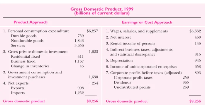
Armed with an understanding of the concepts, we can turn to a look at the actual data in the impor-tant Table 5-6.
Flow-of-Product Approach. Look first at the left side of the table. It gives the upper-loop, flow-of-product approach to GDP. Each of the four major components appears there, along with the produc-tion in each component for 1999. Of these, Cand G
and their obvious subclassifications require little discussion.
DETAILS OF THE NATIONAL ACCOUNTS
99
Gross Domestic Product, 1999 (billions of current dollars)
Earnings or Cost Approach
1. Wages, salaries, and supplements $5,332
2. Net interest 468
3. Rental income of persons 146 4. Indirect business taxes, adjustments,
and statistical discrepancy 815
5. Depreciation 945
6. Income of unincorporated enterprises 658 7. Corporate profits before taxes (adjusted) 893
Corporate profit taxes 259
Dividends 365
Undistributed profits 269 ______ Gross domestic product $9,256
TABLE 5-6. The Two Ways of Looking at the GDP Accounts, in Actual Numbers
The left side measures flow of products (at market prices). The right side measures flow of costs (factor earnings and depreciation plus indirect taxes). (Source: U.S. Department of Commerce.) Product Approach
1. Personal consumption expenditure $6,257
Durable goods 759
Nondurable goods 1,843
Services 3,656
2. Gross private domestic investment 1,623 Residential fixed 411 Business fixed 1,167 Change in inventories 45 3. Government consumption and
investment purchases 1,630
4. Net exports 254
Exports 998
Imports 1,252 ______
Depreciation on capital goods that were used up must appear as an expense in GDP, just like other expenses.
Profit comes last because it is the residual—what is left over after all other costs have been subtracted from total sales. There are two kinds of profits: profit of corporations and net earnings of unincorporated enterprises.
Income of unincorporated enterprises consists of earnings of partnerships and single-ownership busi-nesses. This includes much farm and professional in-come.
Finally, corporate profits before taxes are shown. This entry’s $893 billion in Table 5-6 includes cor-porate profit taxes of $259 billion. The remainder then goes to dividends or to undistributed corporate profits; the latter amount of $269 billion is what cor-porations leave or “plow back” into the business and is called net corporate saving.
On the right side, the flow-of-cost approach gives us the same $9256 billion of GDP as does the flow-of-product approach. The right and left sides do agree.
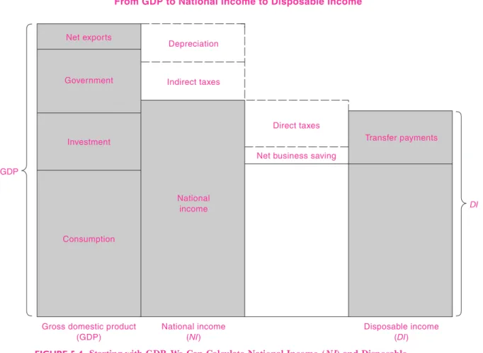
From GDP to Disposable Income
The basic GDP accounts are of interest not only for themselves but also because of their importance for understanding how consumers and businesses be-have. Some further distinctions will help illuminate the way the nation’s books are kept.
National Income. To help us understand the divi-sion of total income among the different factors of production, we construct data on national income (NI ). NIrepresents the total incomes received by la-bor, capital, and land. It is constructed by subtract-ing depreciation and indirect taxes from GDP. Na-tional income equals total compensation of labor, rental income, net interest, income of proprietors, and corporate profits.
The relationship between GDP and national in-come is shown in the first two bars of Figure 5-4. The left-hand bar shows GDP, while the second bar shows the subtractions required to obtain NI.
Disposable Income. A second important concept asks, How many dollars per year do households ac-tually have available to spend? The concept of dis-posable personal income (usually called disposable
Gross private domestic investment does require one comment. Its total ($1623 billion) includes all new business fixed investment, residential construction, and increase in inventory of goods. This gross total ex-cludes subtraction for depreciation of capital. After subtracting $945 billion of depreciation from gross in-vestment, we obtain $678 billion of net investment. Finally, note the large negative entry for net ex-ports, $254 billion. This negative entry represents the fact that in 1999 the United States imported $254 billion more in goods and services than it exported. Adding up the four components on the left gives the total GDP of $9256 billion. This is the harvest we have been working for: the money measure of the American economy’s overall performance for 1999. Flow-of-Cost Approach. Now turn to the right-hand side of the table, which gives the lower-loop, flow-of-cost approach. Here we have all net costs of production
plus taxesand depreciation.
Wages and other employee supplements include all take-home pay, fringe benefits, and taxes on wages. Net interest is a similar item. Remember that interest on government debt is not included as part of Gor of GDP but is treated as a transfer.
Rent income of persons includes rents received by landlords. In addition, if you own your own home, you are treated as paying rent to yourself. This is one of many “imputations” (or derived data) in the national accounts. It makes sense if we really want to measure the housing services the American people are enjoy-ing and do not want the estimate to change when people decide to own a home rather than rent one. Indirect business taxes are included as a separate item along with some small adjustments, including the inevitable “statistical discrepancy,” which reflects the fact that the officials never have every bit of needed data.2
2
Statisticians work with incomplete reports and fill in data gaps by estimation. Just as measurements in a chemistry lab differ from the ideal, so do errors creep into both upper- and lower-loop GDP estimates. These are balanced by an item called the “statistical discrepancy.” Along with the civil servants who are heads of units called “Wages,” “Interest,” and so forth, there actually used to be someone with the title “Head of the Statistical Discrepancy.” If data were perfect, that individual would have been out of a job. In fact, during the late 1990s, income-side GDP grew substantially faster than product-side GDP, and in 1999 the statistical discrepancy was $125 billion. Economists are scratching their heads and trying to deter-mine where all that income was hidden.
income,or DI) answers this question. To get dispos-able income, you calculate the market and transfer incomes received by households and subtract per-sonal taxes.
Figure 5-4 shows the calculation of DI. We begin with national income in the second bar. We then sub-tract all direct taxes on households and corporations and further subtract net business saving. (Business saving is depreciation plus profits minus dividends. Net business saving is this total minus depreciation.) Finally, we add back the transfer payments that households receive from governments. This consti-tutes DI, shown as the right-hand bar in Figure 5-4.
Disposable income is what actually gets into the pub-lic’s hands for consumers to dispose of as they please. As we will see in the next chapters, DIis what peo-ple divide between (1) consumption spending and (2) personal saving.
Saving and Investment
As we have seen, output can be either consumed or invested. Investment is an essential economic activ-ity because it increases the capital stock available for future production. One of the most important points about national accounting is the identity between sav-ing and investment. We will show that, under the
ac-DETAILS OF THE NATIONAL ACCOUNTS
101
GDP
DI
Net business saving Direct taxes Transfer payments National income Indirect taxes Depreciation Net exports Government Investment Consumption
From GDP to National Income to Disposable Income
Gross domestic product (GDP)
National income (NI)
Disposable income (DI)
FIGURE 5-4. Starting with GDP, We Can Calculate National Income (N I) and Disposable Personal Income (D I)
Important income concepts are (1) GDP, which is total gross income to all factors; (2) na-tional income, which is the sum of factor incomes and is obtained by subtracting deprecia-tion and indirect taxes from GDP; and (3) disposable personal income, which measures the total incomes, including transfer payments, but minus taxes, of the household sector.
net exports). The sources of saving are private sav-ing (by households and businesses) and government saving (the government budget surplus). Private in-vestment plus net exports equals private saving plus the budget surplus. These identities must hold al-ways, whatever the state of the business cycle.
BEYOND THE NATIONAL
ACCOUNTS
Advocates of the existing economic and social sys-tem often argue that market economies have pro-duced a growth in real output never before seen in human history. “Look how GDP has grown because of the genius of free markets,” say the admirers of capitalism.
But critics point out the deficiencies of GDP. GDP includes many questionable entries and omits many valuable economic activities. As one dissenter said, “Don’t speak to me of all your production and your dollars, your gross domestic product. To me, GDP stands for gross domestic pollution!”
What are we to think? Isn’t it true that GDP includes government production of bombs and missiles along with salaries paid to prison guards? Doesn’t an increase in crime boost sales of home alarms, which adds to the GDP? Doesn’t cutting our irreplaceable redwoods show up as a positive output in our national accounts? Doesn’t GDP fail to ac-count for environmental degradation such as acid rain and global warming?
In recent years, economists have begun develop-ing new measures to correct the major defects of the standard GDP numbers and better reflect the true satisfaction-producing outputs of our economy. The new approaches attempt to extend the boundaries of the traditional accounts by including important nonmarket activities as well as correcting for harm-ful activities that are included as part of national out-put. Let’s consider some of the omitted pluses and minuses.
Omitted Nonmarket Activities. Recall that the stan-dard accounts include primarily market activities. Much useful economic activity takes place outside the market. For example, college students are investing in human capital. The national accounts record the tuition, but they omit the opportunity costs of earn-ings forgone. Studies indicate that inclusion of non-counting rules described above, measured saving is
ex-actly equal to measured investment. This equality is an
identity, which means that it must hold by definition. In the simplest case, assume for the moment that there is no government or foreign sector. Investment is that part of national output which is not consumed. Saving is that part of national income which is not consumed. But since national income and output are equal, this means that saving equals investment. In symbols:
Iproduct-approach GDP minus C Searnings-approach GDP minus C
But the measures always give the same measure of GDP, so
IS: the identity between measured saving and investment
That is the simplest case. We also need to con-sider the complete case which brings businesses, gov-ernment, and net exports into the picture. On the saving side, total or national saving(ST) is composed of private savingby households and businesses (SP) along with government saving(SG). Government sav-ing equals the government’s budget surplus or the difference between tax revenues and expenditures. On the investment side, total or national invest-ment (IT) starts with gross private domestic investment
(I) but also adds net foreign investment, which is ap-proximately the same as net exports (X). Hence, the complete saving-investment identity is given by3
or
ITIXSPSGST
National saving equals national investment by definition. The components of investment are pri-vate domestic investment and foreign investment (or
National private net
Investment investment exports
private government national
saving saving saving
3 For this discussion, we consider only private investment and therefore treat all government purchases as consumption. In most national accounts today, government purchases are di-vided between consumption and tangible investments. If we include government investment, then this amount will add to both national investment and the government surplus.
market investments in education and other areas would more than double the national saving rate.
Similarly, many household activities produce valuable “near-market” goods and services such as meals, laundering, and child-care services. Recent estimates of the value of unpaid household work in-dicate that it might be almost 50 percent as large as total market consumption. Perhaps the largest omis-sion from the market accounts is the value of leisure time. On average, Americans spend as much of their time on utility-producing leisure activities as they do on money-producing work activities. Yet the value of leisure time is excluded from our official national statistics.
You might wonder about the many activities in the underground economy, which covers a wide va-riety of market activities that are not reported to the government. These include activities like gambling, prostitution, drug dealing, work done by illegal im-migrants, bartering of services, and smuggling. Ac-tually, much underground activity is intentionally ex-cluded because national output excludes illegal activities—these are by social consensus “bads” and not “goods.” A swelling cocaine trade will not enter into GDP. For other, legal but unreported activities, like unreported tips, the Commerce Department makes estimates on the basis of surveys and audits by the Internal Revenue Service.
Omitted Environmental Damage. In addition to omitting activities, sometimes GDP omits some of the harmful side effects of economic activity. An impor-tant example is the omission of environmental dam-ages. For example, suppose the residents of Subur-bia buy 10 million kilowatt-hours of electricity to cool their houses, paying Utility Co. 10 cents per kilowatt-hour. That $1 million covers the labor costs, plant costs, and fuel costs. But suppose the company dam-ages the neighborhood with pollution in the process of producing electricity. It incurs no monetary costs for this externality. Our measure of output should not only add in the value of the electricity (which GDP does) but also subtract the environmental dam-age caused by the pollution (which GDP does not). Suppose that in addition to paying 10 cents of di-rect costs, the surrounding neighborhood suffers 1 cent per kilowatt-hour of environmental damage. This is the cost of pollution (to trees, trout, streams, and people) not paid by Utility Co. Then the total
“external” cost is $100,000. To correct for this hid-den cost in a set of augmented accounts, we must subtract $100,000 of “pollution bads” from the $1,000,000 flow of “electricity goods.”
PRICE INDEXES AND INFLATION
103
Augmented national accounts
Considerable progress has been made in re-cent years in developing augmented national accounts, which are accounts designed to in-clude both nonmarket and market activities.The general principle of augmented accounting is to include as much of economic activity as is feasible, whether or not that activity takes place in the market. Examples of augmented accounts include estimates of the value of non-market investments in human capital, the value of unpaid home production, the value of forests, and the value of leisure time.
In 1994, the U.S. Commerce Department unveiled its augmented national accounts with the introduction of en-vironmental accounts (sometimes called “green accounts”) designed to estimate the contribution of natural and en-vironmental resources to the nation’s income. The first step was the development of accounts to measure the contribution of subsoil assets like oil, gas, and coal.
Environmental critics have argued that America’s wasteful ways are squandering our precious natural capi-tal. Many were surprised by the results of this first assay into green accounting. The estimates take into account that discovery adds to our proven reserves while extraction subtracts from or depletes these reserves. In fact, these two activities just about canceled each other out: the net effect of both discoveries and depletion from 1958 to 1991 was between minus $2 billion and plus $1 billion, depending on the method, as compared to an average GDP over this period of $4200 billion (all these in 1992 prices).
There is much further work needed in this area be-fore we have a full picture of nonmarket economic ac-tivity. Economists and environmentalists are watching this exciting new development carefully.
PRICE INDEXES AND INFLATION
We have concentrated in this chapter on the meas-urement of output. But people are also concerned with price trends, with movements in the overall price level, with inflation. What do these terms mean?portant price indexes are the consumer price index, the GDP deflator, and the producer price index.
The Consumer Price Index (CPI). The most widely
used measure of inflation is the consumer price in-dex, also known as the CPI, calculated by the Bureau of Labor Statistics (BLS). The CPI measures the cost of buying a standard basket of goods at different times. The market basket includes the prices of food, clothing, shelter, fuel, transportation, medical care, college tuition, and other goods and services pur-chased for day-to-day living. Prices on 364 separate classes of goods and services are collected from 23,000 establishments in 87 areas of the country.
How are the different prices weighted in con-structing price indexes? It would clearly be silly merely to add up the different prices or to weight them by their mass or volume. Rather, a price index is constructed by weighting each price according to the economic importance of the commodity in question.
In the case of the traditional CPI, each item is as-signed a fixed weight proportional to its relative im-portance in consumer expenditure budgets; the weights for each item are proportional to the total spending by consumers on that item as determined by a survey of consumer expenditures in the 1993– 1995 period. As of December 1999, housing-related costs were the single biggest category in the CPI, tak-ing up more than 40 percent of consumer spendtak-ing budgets. By comparison, the cost of new cars and other motor vehicles accounts for only 5 percent of the CPI’s consumer expenditure budgets. (We are discussing the “traditional CPI” because the govern-ment is currently in the process of undertaking a fundamental redesign of the methods for calculating the CPI.)
We can use a numerical example to illustrate how inflation is measured. Assume that consumers buy three commodities: food, shelter, and medical care. A hypothetical budget survey finds that consumers spend 20 percent of their budgets on food, 50 per-cent on shelter, and 30 perper-cent on medical care.
Using 1998 as the base year, we reset the price of each commodity at 100 so that differences in the units of commodities will not affect the price index. This implies that the CPI is also 100 in the base year [(0.20100)(0.50100)(0.30100)]. Next, we calculate the consumer price index and the rate of inflation for 1999. Suppose that in 1999 Let us begin with a careful definition:
Aprice indexis a measure of the average level of prices. Inflation denotes a rise in the general level of prices. The rate of inflation is the rate of change of the general price level and is measured as follows:
Rate of inflation (year t)
price level price level
(year t) (year t1)
100
price level (year t1)
But how do we measure the “price level” that is involved in the definition of inflation? The price level is a weighted average of the prices of the dif-ferent goods and services in an economy. The gov-ernment calculates the price level by constructing
price indexes,which are averages of prices of goods and services.
As an example, take the year 1999. In that year, the prices of most major categories rose modestly— food prices rose 2 percent and medical-care prices rose 3.5 percent, for example. Apparel prices de-clined, however, primarily because of sharp declines in the prices of imported clothing. Overall, when weighted by total expenditures in different areas, the consumer price index (CPI) rose 2.1 percent in 1999. In other words, the inflation rate was 2.1 per-cent.
The opposite of inflation is deflation,which oc-curs when the general level of prices is falling. De-flations have been rare in the late twentieth century. In the United States, the last time consumer prices actually fell from one year to the next was 1955. Sus-tained deflations, in which prices fall steadily over a period of several years, are associated with depres-sions, such as those that occurred in the United States in the 1930s and the 1890s. More recently, Japan experienced a deflation in the late 1990s as its economy suffered a prolonged recession.
Price Indexes
When newspapers tell us “Inflation is rising,” they are really reporting the movement of a price index. A price index is a weighted average of the prices of a number of goods and services. In constructing price indexes, economists weight individual prices by the economic importance of each good. The most
im-food prices rise 2 percent to 102, shelter prices rise 6 percent to 106, and medical-care prices are up 10 percent to 110. We recalculate the CPI for 1999 as follows:
CPI (1999)
(0.20102)(0.50106)(0.30110)
106.4
In other words, if 1998 is the base year in which the CPI is 100, then in 1999 the CPI is 106.4. The rate of inflation in 1999 is then [(106.4100)/100] 1006.4 percent per year. Note that in a fixed-weight index like the CPI, the priceschange from year to year but the weights remain the same.
This example captures the essence of how the tra-ditional CPI measures inflation. The only difference between this simplified calculation and the actual one is that the CPI in fact contains many more com-modities and regions. Otherwise, the procedure is exactly the same.
GDP Deflator. Another widely used price index is the GDP deflator, which we met earlier in this chap-ter. The GDP deflator is the price of all goods and services produced in the country (consumption, in-vestment, government purchases, and net exports) rather than of a single component (such as con-sumption). This index also differs from the tradi-tional CPI because it is a variable-weight index that takes into account the changing shares of different goods. In addition, there are deflators for compo-nents of GDP, such as for investment goods, com-puters, personal consumption, and so forth, and these are sometimes used to supplement the CPI. In recent years, the U.S. government has intro-duced chain-weighted price indexes that change the weights on each good each period to reflect changes in expenditure shares (see the discussion of chain weights in note 1 on page 94).
The Producer Price Index (PPI). This index, dating from 1890, is the oldest continuous statistical series published by the BLS. It measures the level of prices at the wholesale or producer stage. It is based on ap-proximately 3400 commodity prices, including prices of foods, manufactured products, and mining prod-ucts. The fixed weights used to calculate the PPI are the net sales of each commodity. Because of its great detail, this index is widely used by businesses.
PRICE INDEXES AND INFLATION
105
Getting the prices right
Measuring prices accurately is one of the cen-tral issues of empirical economics. Price in-dexes affect not only obvious things like the inflation rate. They also are embedded in meas-ures of real output and productivity. And through government policies, they affect monetary policy, taxes, government transfer programs like social security, and many private contracts.
The purpose of the consumer price index is to meas-ure the cost of living. You might be surprised to learn that this is a difficult task. Some problems are intrinsic to price indexes. One issue is the index-number problem, which in-volves how the different prices are weighted or averaged. Recall that the traditional CPI uses a fixed weight for each good. As a result, the cost of living is overestimated com-pared to the situation where consumers substitute rela-tively inexpensive for relarela-tively expensive goods.
The case of energy prices can illustrate the problem. When gasoline prices rose sharply in the 1970s, people tended to cut back on their purchases and buy smaller cars or travel less. Yet the CPI assumed that they bought the same quantity of gasoline even though gasoline prices tripled. The overall rise in the cost of living was thereby exaggerated. Statisticians have devised ways of minimizing such index-number problems by using different weighting approaches, such as chain weighting, discussed above, but government statisticians are just beginning to experiment with these newer approaches for the CPI.
A more important problem arises because of the dif-ficulty of adjusting price indexes to capture the contribu-tion of new and improved goods and services. An example will illustrate this problem. In recent years, consumers have benefited from compact fluorescent lightbulbs; these lightbulbs deliver light at approximately one-fourth the cost of the older, incandescent bulbs.Yet none of the price indexes incorporate the quality improvement. Sim-ilarly, as CDs replaced long-playing records, as cable TV with hundreds of channels replaced the older technology with a few fuzzy channels, as air travel replaced rail or road travel, and in thousands of other improved goods and serv-ices, the price indexes did not reflect the improved quality. Recent studies indicate that if quality change had been properly incorporated into price indexes, the CPI would have risen less rapidly in recent years. This problem is es-pecially acute for medical care. In this sector, reported prices have risen sharply in the last two decades. Yet we
1. The national income and product accounts contain the major measures of income and product for a coun-try. The gross domestic product (GDP) is the most comprehensive measure of a nation’s production of goods and services. It comprises the dollar value of consumption (C), gross private domestic investment (I), government purchases (G), and net exports (X) produced within a nation during a given year. Recall the formula:
GDPCIGX
This will sometimes be simplified by combining pri-vate domestic investment and net exports into total gross national investment (ITIX):
GDPCITG
2. Because of the way we define residual profit, we can match the upper-loop, flow-of-product measurement of GDP with the lower-loop, flow-of-cost measurement, as shown in Figure 5–1. The flow-of-cost approach uses factor earnings and carefully computes value added to
ACCOUNTING ASSESSMENT
This chapter has examined the way economists meas-ure national output and the overall price level. Hav-ing reviewed the measurement of national output and analyzed the shortcomings of the GDP, what should we conclude about the adequacy of our meas-ures? Do they capture the major trends? Are they ad-equate measures of overall social welfare? The an-swer was aptly stated in a review by Arthur Okun:
It should be no surprise that national prosperity does not guarantee a happy society, any more than personal prosperity ensures a happy family. No growth of GDP can counter the tensions arising from an unpopular and unsuccessful war, a long overdue self-confrontation with conscience on racial injustice, a volcanic eruption of sexual mores, and an unprecedented assertion of independence by the young. Still, prosperity . . . is a precondition for suc-cess in achieving many of our aspirations.5
SUMMARY
have no adequate measure of the quality of medical care, and the CPI completely ignores the introduction of new products, such as pharmaceuticals which replace intrusive and expensive surgery.
A panel of distinguished economists led by Stanford’s Michael Boskin (chief economist to President George Bush) recently estimated that the upward bias in the CPI was slightly more than 1 percent per year. This is a small number with large implications. It indicates that our real output numbers may have been overdeflatedby the same amount. If the CPI bias carries through to the GDP defla-tor, then output per worker-hour in the United States has grown at 2 percent per year over the last two decades rather than the 1 percent per year as measured in the of-ficial national accounts.
This finding also implies that cost-of-living adjustments (which are used for social security benefits and in many labor agreements) have overcompensated people for movements in the cost of living. The Boskin panel esti-mated that if the government were to index transfer pro-grams according to their bias estimate rather than using the current CPI, this would by 2008 reduce the govern-ment defict by $180 billion and lower the U.S. national debt by more than $1 trillion over a decade. These find-ings indicate that the economics of accounting and of dex numbers are no longer just abstruse concepts of in-terest only to a handful of technicians. Proper construction of price and output indexes affects our government budg-ets, our retirement programs, and even the way we assess our national economic performance.
In response to its own research and to its critics, the BLS has undertaken a major overhaul of the CPI.The most
important planned change is to fix the index-number prob-lem by replacing the fixed-weight price index with a sys-tem (like the chain weights used in the GDP accounts) that accounts for consumer substitution. Measuring quality change accurately is a much tougher nut and is unlikely to be cracked soon.4
4
See this chapter’s Further Reading section for a symposium on CPI design.
5 The Political Economy of Prosperity(Norton, New York, 1970), p. 124.
FURTHER READING AND INTERNET WEBSITES
107
eliminate double counting of intermediate products. And after summing up all (before-tax) wage, interest, rent, depreciation, and profit income, it adds to this total all indirect tax costs of business. GDP does not include transfer items such as interest on government bonds or welfare payments.
3. By use of a price index, we can “deflate” nominal GDP (GDP in current dollars) to arrive at a more accurate measure of real GDP (GDP expressed in dollars of some base year’s purchasing power). Use of such a price index corrects for the “rubber yardstick” implied by changing levels of prices.
4. Net investment is positive when the nation is produc-ing more capital goods than are currently beproduc-ing used up in the form of depreciation. Since depreciation is hard to estimate accurately, statisticians have more confidence in their measures of gross investment than in those of net investment.
5. National income and disposable income are two ad-ditional official measurements. Disposable income (DI) is what people actually have left—after all tax pay-ments, corporate saving of undistributed profits, and transfer adjustments have been made—to spend on consumption or to save.
6. Using the rules of the national accounts, measured sav-ing must exactly equal measured investment. This is
easily seen in a hypothetical economy with nothing but households. In a complete economy, private saving and government surplus equal domestic investment plus net for-eign investment. The identity between saving and in-vestment is just that: saving must equal inin-vestment no matter whether the economy is in boom or recession, war or peace. It is a consequence of the definitions of national income accounting.
7. Gross domestic product and even net domestic prod-uct are imperfect measures of genuine economic wel-fare. In recent years, statisticians have started correct-ing for nonmarket measures such as unpaid work at home and environmental externalities.
8. Inflation occurs when the general level of prices is ris-ing (and deflation occurs when it is fallris-ing). We meas-ure the overall price level and rate of inflation using price indexes—weighted averages of the prices of thousands of individual products. The most important price index is the consumer price index (CPI), which traditionally measured the cost of a fixed market bas-ket of consumer goods and services relative to the cost of that bundle during a particular base year. Recent studies indicate that the CPI trend has a major upward bias because of index-number problems and omission of new and improved goods, and the government has undertaken steps to correct some of this bias.
Websites
The premium site for the U.S. National Income and Prod-uct Accounts is from the Bureau of Economic Analysis (BEA) at www.bea.doc.gov. This site also contains recent issues of The Survey of Current Business, which discusses re-cent economic trends.
national income and product accounts (national accounts) real and nominal GDP
GDP deflator
GDPCIGX
net investment
gross investmentdepreciation
GDP in two equivalent views: product (upper loop) earnings (lower loop)
intermediate goods, value added NDPGDPdepreciation government transfers disposable income (DI) investment-saving identity IS ITIXSPSGST inflation, deflation price index: CPI GDP deflator PPI
FURTHER READING AND INTERNET WEBSITES
Further ReadingA magnificent compilation of historical data on the United States is contained in Historical Statistics of the United States (Washington, D.C., Government Printing Office, 1975, two volumes). A review of the issues involving measuring the consumer price index is contained in “Symposium on the CPI,” Journal of Economic Perspectives, Winter 1998.