Single Channel Sound Source Separation Combining Delay Estimation and the AdRess Algorithm

(1)

Technological University Dublin

ARROW@TU Dublin

Conference papers

Audio Research Group

2008-01-01

Single Channel Sound Source Separation Combining Delay

Estimation and the AdRess Algorithm

Mark Leddy

Technological University Dublin

Dan Barry

Technological University Dublin, [email protected]

David Dorran

Eugene Coyle

Follow this and additional works at: https://arrow.tudublin.ie/argcon Part of the Other Engineering Commons

Recommended Citation

Leddy, M., Barry, D., Dorran, D. & Coyle, E. Single channel sound source separation combining delay estimation and the AdRess algorithm. Paper given at the Irish Signals and Systems Conference, National University of Galway, 2008. http://www.audioresearchgroup.com/

This Conference Paper is brought to you for free and open access by the Audio Research Group at

ARROW@TU Dublin. It has been accepted for inclusion in Conference papers by an authorized administrator of ARROW@TU Dublin. For more information, please

contact [email protected],

[email protected], [email protected].

This work is licensed under a Creative Commons

(2)

ISSC 2008, Galway, June 18–19

Single Channel Sound Source Separation combining

Delay Estimation and the ADRess algorithm

Mark Leddy, Dan Barry, David Dorran and Eugene Coyle.

Audio Research Group

Dublin Institute of Technology, Kevin St.,

IRELAND

E-mail:

[email protected]

Abstract —A method for single channel source separation is proposed in this paper, which uses estimates of the delay co-efficient of individual sources within an echoic mixture using autocorrelation, following which a “pseudo-stereo mixture” is generated, to which the ADRess algorithm can be applied. The system is evaluated in a theoretical situation, where the mixture signal to be separated consists of two individual source signals, and a delayed version of each signal. Estimates of the individual delay lengths are made and then used to create a pseudo stereo mix, where one channel consists of the original mixture signal, and the second channel consists the original mixture signal shifted by the length of the delay calculated for each source. The ADRess algorithm is then used to separate sources from the new pseudo stereo mixture.

Keywords—Single channel, Blind Source Separation, ADRess, BSS

I Introduction

Sound source separation is the process of sepa-rating individual source signals from a mixture of multiple sources. Techniques such as DUET [3], and ADRess [2] are used to perform source sep-aration, however they require the use of at least two different mixtures of the same sources. In the case of audio separation, two microphones or a two channel recording are required. These techniques have been shown to work well and can produce robust and high-quality results.

Factorisation based approaches such as PCA [7], ICA [6] and NMF [4] have been applied using just a single mixture of sources. These techniques have shown their effectiveness for certain tasks such as musical transcription. However, in general, the output resynthesis quality of the separations are not as robust as the above 2-channel techniques.

Proposed here is a source separation technique, which creates a two-channel, pseudo-stereo mix-ture from a single-channel mixmix-ture signal. From this stereo mixture the ADRess algorithm can be employed to separate a single source from the

mix-ture. By using this technique it is shown that ro-bust separation results from just a single channel mixture signal is possible.

The aim of this paper is to show that the de-scribed technique will work for simplified, syn-thetic cases, in order to pave the way for further exploration.

II Delay Model

The theoretical model, used to represent a single source in an echoic environment, is illustrated in

Fig. 1. Here S represents a source signal that is

transmitted. Acoustic pressure waves will travel along a direct path, to the sensor, and also re-flected paths, rebounding off surfaces, before

ac-cumulating at the target sensor x. This mixture

model is represented in equation (1) [9]. x(t) =

N X

i

αis(t+ ∆ti) (1)

where αi ≥0 represents the attenuation over the

(3)

x R1 R₂ R3 d s

Fig. 1: Figure shows the direct pathd, from the sources, to the sensorx. The three reflected pathsRiare also

shown. Due to the extra distance traversed to reach the sensor, eachRiwill be attenuated compared to the direct

path. Similarly, due to the extra time taken to travel the the reflected paths, upon reaching the sensor they will

appear as delayed versions of the source.

Ri, in comparison to the direct path d, as

illus-trated in Fig. 1. Riis the path travelled by signals

to reach the sensor along the ith _{reflected path,}

anddis the path taken by the signal, to reach the

sensor along the direct path. The resulting delay due to the extra time required to traverse the re-flected path, compared to that of the direct path, (Ri−d), is represented by ∆ti.

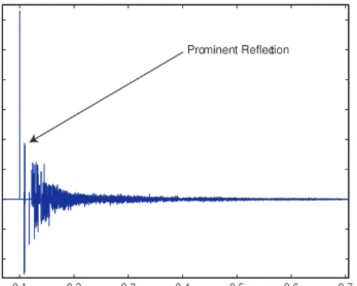
In reality, an infinite number of possible reflec-tions will be present in an echoic environment. Typically however, many environments will have a small number of strong reflections. This is il-lustrated by measuring the impulse response of an echoic environment, see Fig. 2. However, for the purposes of this paper, a simplified situation will be demonstrated. 0.1 0.2 0.3 0.4 0.5 0.6 0.7 0.2 0.1 0 0.1 0.2 0.3 0.4 0.5 0.6 Time (seconds) Typical Impulse Response

Prominent Reflection

Fig. 2: Typical Impulse Response of an echoic environment. A prominent reflection can clearly be distinguished. If these reflections can be estimated, separation may be possible using the technique described

in this paper.

The simplified situation presented in this paper assumes that only two sources are present, and that each source is only reflected once. This situa-tion is presented in Fig. 3, the model described in

equation (2) is used.

x(t) = [s1(t) +αs1(t+ ∆t1)] +...

+[s2(t) +βs2(t+ ∆t2)] (2)

wheresi(t) represents sources received by the

sen-sor at time t. The value ∆ti represents the extra

time taken for a reflected signal to reach the sensor. The attenuation coefficients of the first and second signals, having travelled the extra reflected dis-tance before reaching the sensor, are represented

byαandβrespectively. Hence the sensor mixture

will consist of each source, and one delayed and attenuated version of each source.

x d(s1) s1 s2 d(s2) R(s1) R(s2)

Fig. 3: Theoretical model used to illustrate the situation in which source separation will be performed. The system

contains 2 sourcessi. Each will take a direct path,d(si)

to the sensorx, and also a reflected pathR(si).

III Auto-Correlation and Stereo

alignment

Autocorrelation, is used estimate the delay

coeffi-cients ∆tipresent in the mixture signalx(t),

equa-tion (3). Rm(k) =

N_X−1

j=0

x(t+j)x(t) (3)

where N is the length of the mixture signal x(t).

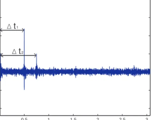
Autocorrelation can be used to find periodic or re-peating patterns within the signal. Applying auto-correlation to the mixture signal will give an

esti-mation of the length of the delays ∆t1and ∆t2, see

Fig. 4. The autocorrelation function here shows two significant peaks which indicate time delays

∆t1 and ∆t2. It is difficult to distinguish which

delay belongs to which source at this point. Once the delay coefficient has been established a second channel is created. This will consist of the original mixture signal, shifted forward in time by

the estimated delay coefficient ∆ti. The delayed

and attenuated version of theith _{source, will then}

be time-aligned with the ‘original’ source within the mixture. This results in a two channel mixture, consisting ofx(t) andx(t−∆ti), which will be used

to recover the ith_source.

In theory, it should be possible to separate sin-gle sources, from a mixture of a large number of

(4)

0.5 1 1.5 2 2.5 3 400 200 0 200 400 600 800 Time (seconds) Estimates of delay coefficients

∆t1

∆t2

Fig. 4: Autocorrelation of the mixture signals. The peaks are used to estimate the delay coefficients ∆ti.

sources. What limits this, is the increased diffi-culty associated with measuring the delay coeffi-cients using autocorrelation. As long as accurate estimates can be found, such as those in Fig. 4,

it should be possible to perform separation for n

sources. However as n increases, time-frequency

overlap will reduce the resynthesis quality attain-able with ADRess.

IV Stereo Space Source Separation

Having aligned the mixture signals into a pseudo-stereo, two-channel mixture, the ADRess algo-rithm can be used to separate the desired source signal. Taking a stereo mixture, the ADRess al-gorithm separates sources according to their lat-eral displacement within a stereo field. A stereo localisation, or lateral displacement effect, occurs when there is a difference in the intensity of a single source between each channel. This intensity differ-ence allows for the creation of a histogram repre-senting the stereo space, where by the position of sources within the stereo field can be located.

In order for ADRess to operate, the linear in-tensity mixing model must apply. Essentially; the sources for separation in the left and right mixture must be phase coherent, ie. time aligned. The lateral displacement must only be a function of in-tensity difference between each channel. The time alignment procedure and pseudo stereo mixture creation, attempts to satisfy these criteria. For further information about ADRess, see [2].

By taking our mixture signal x(t) as one

chan-nel, andx(t−∆ti) as a second, the ADRess

algo-rithm can then be applied. Our sourcesi(t), and

its delayed version αsi(t+ ∆ti), have now been

aligned in time. If the attenuation coefficient is

negligible, ieα= 1, then the sourceiwill have the

same intensity in both channels, and hence will be located in the center of the stereo field. Generally the attenuation coefficient of the delayed source is

< 1, and this will cause the source to be located

in the left half of the stereo energy histogram. The ADRess algorithm allows for real-time plot-ting of this histogram. This permits the localisa-tion of the source, and allows the user to choose the correct attenuation factor manually, as indi-cated by a peak on the histogram.

V Testing

In order to test the systems effectiveness, speech signals were used rather than musical signals. Speech signals display approximate W-disjoint or-thogonality [5], which means the time-frequency representations of the signals do not excessively overlap.

Conversely, it is the nature of musical signals to harmonically overlap. For this reason multiple sources may contribute to a single time frequency point. Also pitched musical notes, for example a note played on a piano, will often tend to last longer than an utterance of speech.

These attributes of musical signals may make it more difficult to get an accurate delay estimate us-ing auto-correlation. Also the stationary length of musical signals, or the amount of time a note per-sists, will typically be longer than the delay coeffi-cient of the first reflection see Fig. 6. If this is the case, the musical sound, and its delayed equivalent will be added together, causing an increase in the magnitude where they overlap. This new magni-tude will cause the intensity to vary erratically, es-sentially causing the attenuation estimate to vary

also. The stationary length of speech is usually

∆ti

x(t) shifted forward by∆ti to

create second channel of pseudo stereo mixture

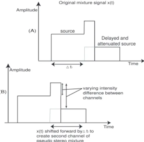
intensity difference between channels Original mixture signal x(t) Amplitude Amplitude Time Time source Delayed and attenuated source (A) (B)

Fig. 5: Illustrates the situation when the stationary length of a signal is<∆ti, the intensity difference will be

constant. This allows robust separation using the ADRess algorithm. (A) denotes the original mixture signalx(t).

(B) represents the newly created channel,x(t−∆ti),

consisting of the original mixture signal, shifted by the estimated delay.

(5)

∆ti

x(t) shifted forward by∆ti to create second channel of pseudo stereo mixture

varying intensity difference between channels Original mixture signal x(t) Amplitude Amplitude Time Time source Delayed and attenuated source (A) (B)

Fig. 6: Illustrates that when the stationary length of a signal is>∆ti, the intensity difference may vary. This

will mean that theith_{signal will be spread over a large}

region of the stereo space, resulting in poorer separation with the ADRess algorithm. (A) denotes the original mixture signalx(t). (B) represents the newly created channel,x(t−∆ti), consisting of the original mixture

signal, shifted by the estimated delay.

this technique is developed with speech separation in mind. For illustrative purposes, two test sig-nals are used in this paper. Each is approximately 7 seconds of male and female speech respectively, see Fig. 8.

VI Results

The test signal used here for illustration, is a sin-gle channel mixture signal, of the form described by equation (2), see Fig. 7. The system was tested by employing 50 linearly spaced delay values, be-tween 0 and 500milliseconds, and testing the sys-tems ability to separate the male voice from the mixture described.

As a performance measurement, the signal to interference ratio (SIR), suggested in [8] is used. This measure was chosen as the model will con-tain no noise, and the only error in the estimation

of the source signalsi(t), will be the contribution

of the other sourcesj(t), and the reflected signals

si(t+ ∆ti) and sj(t+ ∆tj), ∀i 6= j. The SIR is

determined both pre-separation, equation (4), and post-separation, equation (5). Their respective dif-ferences are then used to indicate the level of noise rejection achieved using the technique described here.

SIRpre:= 20 log10||Smixture||Starget−Starget|| || (4) SIRpost:= 20 log10||Sestimate||Sestimate−Starget|| || (5)

whereStarget is the test signal to be separated,

Sestimate represents the separated estimation of

0 1 2 3 4 5 6 7 8 9 −1 −0.8 −0.6 −0.4 −0.2 0 0.2 0.4 0.6 0.8 1 Mixture signal Time (seconds)

Fig. 7: Mixture signal consisting of male speech sample, female speech sample, and an attenuated and delayed

version of each. 0 2 4 6 8 −1 −0.5 0 0.5 1

Male speech sample

0 2 4 6 8 −1 −0.5 0 0.5 1

Estimate of male sample

0 2 4 6 8 −1 −0.5 0 0.5 1

Female speech sample

0 2 4 6 8 −1 −0.5 0 0.5 1

Estimate of female sample

Fig. 8: Male(top left), and Female(top right), Male and Female estimates (bottom left and right respectively).

the target signal. Smixtureis the mixture of signals

represented by equation (2).

Prior to separation, the mixture signal was

gen-erated such that the interfering sources are 4dB

louder than the source of interest, leading to a

sig-nal to noise ratio of−4dB. After applying the

pro-cess described in this paper, analysis shows that

an average of +4dB of signal to interference ratio

has been achieved, resulting in an average signal

to noise ratio increase of 8dB.

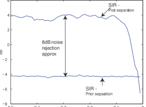
SIRpostfor a delay coefficient from 0.5 to 0.1

sec-onds averages about +4dB. For this delay

time-frame, an approximate +8dB noise rejection

dif-ference is maintained over SIRpre. As the

de-lay coefficient decreases below 0.1 seconds SIRpost

diminishes. However, even though SIRpost

de-creases, the separated signal maintains intelligibil-ity, depending on the source signals, up to around

(6)

0 0.1 0.2 0.3 0.4 0.5 8 6 4 2 0 2 4 6

Signal to interference ratio

Delay coefficient (Seconds)

dB SIR -Post separation SIR - Prior separation 8dB noise rejection approx

Fig. 9: The Signal to interference ratio (SIR) of the target source prior separation, SIR of the estimated source post separation over a varying delay from 0.5 to zero seconds.

VII Conclusion

This paper presented a novel approach to single channel source separation. It has been demon-strated that under simplified conditions, the the-ory can be applied with promising results. Fur-ther work must be undertaken to ascertain how robust the technique will be under less confined constraints, such as a greater number of sources and more realistic acoustic circumstances.

VIII Acknowledgments

Work supported by European Community under the Information Society Technologies (IST) pro-gramme of the 6th FP for RTD - project EASAIER contract IST-033902.

References

[1] P. L. Montgomery. “Modular multiplication

without trial division”. Math. Computation,

44:519–521, 1985.

[2] Barry, D., Lawlor, B., Coyle, E. “Real-time Sound Source Separation: Azimuth Discrimi-nation and Resynthesis”, AES 2004.

[3] S. Rickard, R. Balan, and J. Rosca, “Real-time “Real-time-frequency based blind source

separa-tion,”in 3rd International Conference on

Inde-pendent Component Analysis and Blind Source Separation, San Diego, CA, December 9-12 2001.

[4] Lee, D., Seung, H. “Algorithms for

Non-negative Matrix Factorization”, Adv. Neural

Info. Proc. Syst. , 13, 556-562, 2001.

[5] Jourjine, A., Rickard, S., Yilmaz, O.

“Blind Separation of Disjoint orthogonal sig-nals: Demixing N sources from 2 mixtures”,

ICASSP, 2000.

[6] Hyv¨arinen, A., Erkki, Oja. “Independent

Component Analysis: Algorithms and

Applica-tions”,Neural Networks, 13(4-5):411-430,2000.

[7] Stautner, J.P., “Analysis and Synthesis of

Mu-sic using the Auditory” Transform”, Masters

Thesis, MIT EECS Department, 1983

[8] E. Vincent, R. Gribonval, and C. Favotte,. “Performance Measurement in Blind Audio

Source Separation”. IEEE Transactions on

Speech and Audio Processing, 2005.

[9] Lin, Y., Lee, D. D. and Saul, L. K. “Nonneg-ative deconvolution for time of arrival

estima-tion.”.In Proceedings of the international

Con-ference of Speech, Acoustics, and Signal Pro-cessing (ICASSP-2004), volume 2, pages 377-380, Montreal, Canada, 2004.