The integration of nature-inspired algorithms with Least Square Support Vector regression models: application to modeling river dissolved oxygen concentration

(1)

water

Article

The Integration of Nature-Inspired Algorithms

with Least Square Support Vector Regression

Models: Application to Modeling River Dissolved

Oxygen Concentration

Zaher Mundher Yaseen1ID_{, Mohammad Ehteram}2_{, Ahmad Sharafati}3_{, Shamsuddin Shahid}4 ID_, Nadhir Al-Ansari5,* and Ahmed El-Shafie6ID

1 _{Sustainable Developments in Civil Engineering Research Group, Faculty of Civil Engineering,} Ton Duc Thang University, Ho Chi Minh City, Vietnam; [email protected]

2 _{Department of Water Engineering and Hydraulic Structures, Faculty of Civil Engineering,} Semnan University, Semnan 35131-19111, Iran; [email protected]

3 _{Civil Engineering Department, Science and Research Branch, Islamic Azad University, Tehran, Iran;} [email protected]

4 _{School of Civil Engineering, Universiti Teknologi Malaysia (UTM), Johor Bahru 81310, Malaysia;} [email protected]

5 _{Civil, Environmental and Natural Resources Engineering, Lulea University of Technology,} 97187 Lulea, Sweden

6 _{Civil Engineering Department, Faculty of Engineering, University of Malaya,} Kuala Lumpur 50603, Malaysia; [email protected]

* Correspondence: [email protected]; Tel.: +46-920-491858

Received: 5 July 2018; Accepted: 20 August 2018; Published: 23 August 2018

Abstract: The current study investigates an improved version of Least Square Support Vector Machines integrated with a Bat Algorithm (LSSVM-BA) for modeling the dissolved oxygen (DO) concentration in rivers. The LSSVM-BA model results are compared with those obtained using M5 Tree and Multivariate Adaptive Regression Spline (MARS) models to show the efficacy of this novel integrated model. The river water quality data at three monitoring stations located in the USA are considered for the simulation of DO concentration. Eight input combinations of four water quality parameters, namely, water temperature, discharge, pH, and specific conductance, are used to simulate the DO concentration. The results revealed the superiority of the LSSVM-BA model over the M5 Tree and MARS models in the prediction of river DO. The accuracy of the LSSVM-BA model compared with those of the M5 Tree and MARS models is found to increase by 20% and 42%, respectively, in terms of the root-mean-square error. All the predictive models are found to perform best when all the four water quality variables are used as input, which indicates that it is possible to supply more information to the predictive model by way of incorporation of all the water quality variables. Keywords:dissolved oxygen concentration; LSSVM-BA model; water quality management

1. Introduction

Assessment of river water quality is a challenging issue in field environmental modeling. Among the river water quality parameters, dissolved oxygen (DO) is a critical one for decision-makers in management of water quality and river ecology [1]. The level of DO concentration within a water body (e.g., river and lake) is very important for aquatic organisms (e.g., fish and plants) as low and high values of DO are harmful for the aquatic environment [2]. DO is released within a river through diffusion or aeration processes and by photosynthesis of plants such as algae and phytoplankton [3].

(2)

The sources for supplying DO are limited and, therefore, the conscious management of water quality is very important for maintaining the DO level in water bodies [4].

The DO concentration in a river depends on many biotic/abiotic parameters such as the amount of aquatic plants, nutrient concentrations, streamflow discharge, specific conductance, pH, and water temperature [5], as well as their complex interactions [6]. Physical-based models such as QUAL2K [7] and Water Quality Analysis Simulation Program WASP [8] are generally used to mimic these physical processes in a simplified manner for the prediction of DO. However, the physically based models developed using deterministic equations often fail to predict DO concentration with reasonable accuracy. This is due to several causes: (1) knowledge of many of the biotic/abiotic processes responsible for DO concentration in water bodies is still not clear and the data/information required for modeling many of the interactions are difficult to acquire; (2) many of the biotic/abiotic processes are highly nonlinear and cannot be described perfectly with mathematical equations and (3) hydro-biological data are often prone to errors which cause high uncertainties in prediction [9,10]. However, it has been noticed that many of these processes follow a stochastic behavior. The DO concentration in water bodies changes with time with a sequential relationship between two consecutive values. This encouraged the development of stochastic models in which statistical methods are used to find a relationship between input and output.

The DO concentration in a water body fluctuates on an annual, monthly, daily, or even hourly scale with respect to the water temperature and other features of the water body [4]. Studying the daily and hourly fluctuations of DO concentration might be of interest for particular water bodies with shallow water depth as the concentration of DO fluctuates significantly within a very short period due to high dynamics of physical, chemical, and biological processes in water bodies with shallow depth [9,10]. On the other hand, fluctuation of DO concentration in a river is not significant at the hourly or daily scale. Furthermore, the monthly DO concentration provides seasonal variation of this important water quality parameter which is more useful for management of river water quality and ecology. Therefore, models have been developed in this study for the prediction of the monthly concentration of DO in river.

Regression models are most widely used for modeling stochastic behavior of DO concentration in water bodies [5,11]. Zounemat-Kermani and Scholz (2014) used stepwise regression for the selection of influential parameters for prediction of DO concentration. Khan and Valeo (2015) introduced fuzzy linear regression to predict DO from abiotic factors [5]. Li et al. (2017) employed linear regression for estimation of DO from multiple water quality parameters [12]. However, the capability of conventional regression-based models is limited in simulating highly nonlinear and nonstationary behavior. The time series of DO concentration is often found to be highly stochastic in nature, which is not possible to simulate using conventional regression models. With the advances of artificial intelligence (AI)-based methods, the application of AI in the development of stochastic models has gained significant attention. In recent years, a large number of AI approaches such as artificial neural networks (ANNs), support vector machines (SVMs), fuzzy methods, and model trees (MTs) have been widely used for prediction of different hydrological phenomena such as rainfall [13,14], temperature [15,16], evaporation [17], streamflow [18–20], and water demand [21]. Despite various limitations, the AI-based models have been found to provide hydrological prediction in an efficient way. The AI-based models have simple structure and a low number of mathematical parameters but can consider a large number of predictors. The computational time of AI-based models is much less compared with physical-based models. Furthermore, the AI-based approaches have been found to be highly adaptable to different hydrological and ecological conditions [19]. All these traits give the AI techniques great potential for the modeling of river DO concentration [20].

The AI techniques used for modeling DO concentration can be broadly divided into four groups [22,23]: (i) ANN [1,12,24–33]; (ii) SVM [22,34–37]; (iii) fuzzy logic [5,38–41] and (iv) heuristic models [37,42–45]. Among these, the ANN-based models have been most widely utilized compared with others for the prediction of river DO concentration. Heddam [33] utilized a generalized

(3)

Water2018,10, 1124 3 of 21

regression neural network (GRNN) for predicating DO concentration. He compared the performance of GRNN with multiple linear regressions (MLR) and showed the better prediction capability of GRNN compared with MLR. Nemati et al. [43] compared the performance of an adaptive neuro-fuzzy inference system (ANFIS) and genetic programming (GP) for prediction of DO concentration in a river in Hong Kong and found ANFIS to be more efficient compared with GP in predicting DO concentration. Mohammadpour et al. [45] used a feedforward backpropagation neural network (BPNN) for the prediction of DO concentration. They improved the model performance through optimization of BPNN parameters using particle swarm optimization (PSO) and compared the results with those obtained using SVM. Based on the root mean square error (RMSE) values, they reported that ANN-PSO has higher prediction capability than SVM. Heddam [32] compared the performance of a multilayer perceptron neural network (MPNL) with SVM and least square SVM (LSSVM) for the estimation of river DO concentration and showed superior performance of MPNL compared with SVM and LSSVM. Ay and Kisi [28] and Akkoyunlu et al. [27] used multilayer perceptron neural networks (MLPNNs) and radial basis function neural networks (RBFNNs) to predict DO concentration in USA and Turkey, respectively, and showed their efficiency. Bayram et al. [29] compared the regression and teaching–learning-based optimization approaches to estimate DO concentration in Turkey by employing temperature of air and water as predictors and indicated improvement in model performance through optimization. Kisi et al. [42] assessed the performance of MLPNN, GP, and ANFIS in predicting DO concentration and showed that GP is more capable than others in terms of prediction accuracy.

Besides ANNs, SVMs have also been extensively employed for prediction of river DO concentration [46–48]. Liu et al. [34] optimized the parameters of SVM using PSO to develop an SVM-PSO model for the prediction of DO concentration. They compared the results of SVM-PSO with those of ANN and GP and reported better performance of SVM-PSO. Liu et al. [35] improved the accuracy of LSSVM in the prediction of DO concentration by developing an LSSVM-PSO model and showed that the LSSVM-PSO is more accurate than LSSVM in prediction of DO concentration. Malek et al. (2014) assessed the performance of SVM in the prediction of DO concentration in two different lakes in Malaysia and reported that SVM models using dichotomized values of DO can provide high prediction accuracy [49]. Jadhav et al. compared the performance of LSSVM and GP for estimation of DO concentration in a lake in India and reported similar capabilities of both GP and LSSVM in prediction [37]. An excellent employment of LSSVM for prediction of DO in crab ponds of China was conducted by [50]; the authors found higher accuracy of LSSVM compared with RBFNN. Recently, a new study compared the performance of LSSVM, multivariate adaptive regression splines (MARS), and M5 model trees in the prediction of DO concentration and reported the performance of LSSVM as being very close to that of MARS [51].

The studies revealed the superiority of different AI methods in predicting DO concentration under different environmental conditions. Most of the SVM-based approaches revealed LSSVM as a useful method for estimation of the water quality parameters. However, all the studies reported that the efficiency of LSSVM models significantly depends on the values of the kernel (σ) and regularization (γ) parameters. These hyper-parameters can be considered as decision variables and should be determined accurately by optimization algorithms for better performance of LSSVM models. A number of studies employed different optimization techniques for estimation of optimum values of LSSVM parameters including heuristic optimization approaches such as GA [52–54], PSO [34,55–59], and Colony [60,61] algorithms. In this study, the hyper-parameters of LSSVM were optimized using the Bat algorithm (BA). The proposed hybrid metaheuristic LSSVM-BA algorithm is used for the prediction of DO concentration. The BA has been widely utilized for parameter optimization of the model used in forecasting climatological variables [62,63] and reservoir operation [64,65]. The studies reported BA as an efficient optimization technique. Therefore, it is expected that optimization of LSSVM parameters using BA would significantly improve the prediction capability of LSSVM and the LSSVM-BA model can be used for better prediction of DO concentration in water bodies.

(4)

The main objective of this study is to evaluate the capability of the hybrid metaheuristic LSSVM-BA model in the estimation of monthly DO concentration at three locations of the USA, which has been previously investigated using different AI-based approaches [24,32,33]. The results obtained using LSSVM-BA are compared with those obtained using M5 and MARS. M5 and MARS have been used for the comparison of the performance of LSSVM-BA as they have been found to be highly efficient in the prediction of hydrological variables in a number of recent studies [51,66]. Heddam and Kisi (2018) employed both MARS and M5 for the prediction of DO concentration at the same locations to compare their performance with LSSVM [51]. Therefore, comparison of performance of LSSVM-BA with MARS and M5 will help to assess the improvement of the performance of LSSVM after integration with BA.

2. Materials and Methods 2.1. LSSVM

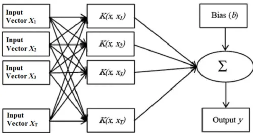
LSSVM [59] is an edited version of SVM [67]. The SVM acts based on a set of quadratic programming problems [68] while the LSSVM acts based on linear programming and linear equations to improve the performance of the SVM. A nonlinear mapping function is used in LSSVM (Figure1) which is based on following Equations (1) and (2) [69]:

f(x) =wTϕ(x) +b (1)

whereϕ(x)is a nonlinear function used for the mapping of the input variables to a higher-dimensional space,wTis the weight vector, andbis the bias term. The values ofbandwTare computed using the following cost function:

CF= 1 2w T_w₊1 2γ N

∑

i=1 e2_i (2)

The following constraints are considered for the cost function:

yi=wTϕ(xi) +b+ei (3)

whereγis the regularization parameter;Nis the number of datapoints;xiandyiare the parameters

which are defined as input parameter (pH, temperature, depth sensor, and other parameters) and output parameter (DO concentration), respectively; andeiis the residual vector for the input data.

A kind of convex optimization problem is generated based on Equations (3) and (4) which is solved by the Lagrange Multipliers method based on the following equation:

L(w,b,e,α) =1 2w T_w₊1 2γ N

∑

i=1 e2_i − N

∑

i=1 αi wTϕ(xi) +b+ei−yi (4) whereα is the Lagrange Multiplier and the following equation is computed based on the partial derivative of Equation (5) with consideration ofw,b,e,α[69]:

y= N

∑

i=1 αiϕ(x)ϕ(xi) +b= N

∑

i=1 αi(ϕ(x)ϕ(xi)) +b (5)

The kernel function is defined based on the following equation:

(5)

Water2018,10, 1124 5 of 21

Then, Equation (7) is inserted into Equation (6) and the following equation is generated: K(x,xi) =exp _−k x−xik 2σ2 (7) y= N

∑

i=1 αik(x,xi) +b (8)

There are several kinds of kernel functions which can be used. Previous studies showed that the radial basis function has the better performance [24] and, thus, it is used in this study:

K(x,xi) =exp _−k_x₋_x ik 2σ2 (9) Theσandγare important parameters which have a significant impact on the final results. In the present study, the values of these parameters are inserted into the bat algorithm as decision variables in order to obtain the optimum values.

Water 2018, 10, x FOR PEER REVIEW 5 of 21

There are several kinds of kernel functions which can be used. Previous studies showed that the radial basis function has the better performance [24] and, thus, it is used in this study:

(

,

)

exp ₂ 2 i i x x K x x

σ

− −  =     (9)

The σ and γ are important parameters which have a significant impact on the final results. In the present study, the values of these parameters are inserted into the bat algorithm as decision variables in order to obtain the optimum values.

Figure 1. Diagram showing the structure of a typical Least Square Support Vector Machine (LSSVM) model.

2.2. Bat Algorithm

The bat generates a loud sound which is returned back through reflection from surrounding objects including its prey. Based on this echolocation ability, the bat can identify its prey. The following assumptions are considered in the bat algorithm [70]:

i. All bats use the echolocation ability for the identification of prey based on received sounds from the surroundings.

ii. Each bat has random velocity ( ) at the position and the loudness, wavelength, and frequency of received sounds are , , and , respectively.

iii. The loudness varies from a large positive value to a minimum value.

The bats have the pulsation rate which varies from 0 to 1, where 0 means the pulsation rate has reached its minimum, while 1 means it has reached its maximum. The velocity, frequency, and position values for bats are updated based on the following Equations (10)–(12):

(

)

min max min l f = f + f − f ×β (10)

( )

1 l l l v t =_y t− −Y_∗_×f (11)

( )

1

( )

l l l y t = y t− +v t ×t (12) where, ( − 1) is the position at time t − 1, is a random vector between 0 and 1, is the minimum frequency, is the maximum frequency, ∗ is the best location for bats, t means time step, and ( ) indicates the velocity for bats. Then, local search based on a random walk is considered based on the following equation:

Figure 1. Diagram showing the structure of a typical Least Square Support Vector Machine (LSSVM) model.

2.2. Bat Algorithm

The bat generates a loud sound which is returned back through reflection from surrounding objects including its prey. Based on this echolocation ability, the bat can identify its prey. The following assumptions are considered in the bat algorithm [70]:

i All bats use the echolocation ability for the identification of prey based on received sounds from the surroundings.

ii Each bat has random velocity (vl) at the positionyland the loudness, wavelength, and frequency

of received sounds areAo,λ, andfmin, respectively.

iii The loudness varies from a large positive value to a minimum value.

The bats have the pulsation rate which varies from 0 to 1, where 0 means the pulsation rate has reached its minimum, while 1 means it has reached its maximum. The velocity, frequency, and position values for bats are updated based on the following Equations (10)–(12):

fl = fmin+ (fmax−fmin)×β (10)

(6)

yl(t) =yl(t−1) +vl(t)×t (12)

where,yl(t−1)is the position at timet−1,βis a random vector between 0 and 1, fminis the minimum

frequency, fmaxis the maximum frequency,Y∗is the best location for bats,tmeans time step, andvl(t)

indicates the velocity for bats. Then, local search based on a random walk is considered based on the following equation:

y(t) =y(t−1) +εA(t) (13)

whereA(t)is loudness andεis a random number between−1 and 1.

The loudness and pulsation rate are updated at each level. When the bats find the prey, the loudness value decreases and the pulsation rate increases based on Equation (14):

r_lt+1=r0_l[1−exp(−γt)]At_l+1=αAt_l (14) whereγandαare constant parameters.

2.3. LSSVM-BA Algorithm

The bats’ positions are considered as decision variables and the values ofσ

andγare the LSSVM parameters which need to be optimized based on an objective function such as RMSE estimated from simulated DO and measured DO values. The improvement of LSSVM in the current study is done based on the following steps:

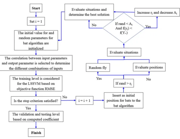
• The initial values for the random parameters in the bat algorithm andσandγparameters are initialized in the first level.

• A counter number is considered for this level, such as in Figure2.

• The kind of kernel function and the inputs and output are selected and the correlation between inputs and output is measured to determine the effective combination of inputs.

• The model is trained, and the performance of the method is evaluated based on objective function such as RMSE.

• The stop criterion is checked and if it is satisfied, the algorithm is shifted to the validation and testing phases and the results based on extracted parameters ofγandαare considered for making a decision on the continuation of the method.

• The values ofγandαas initial positions of bats are inserted into the bat algorithm. In fact, they are considered as decision variables.

• If rand >rlis considered, the positions based on objective functions are evaluated; otherwise,

the random fly is considered and shifted to the next level.

• If rand <Al andf(yl) < f(Y∗)is considered, therlis increased and Alis decreased; otherwise,

the bats’ situations are evaluated and switched to next level.

• One number is added to the counter and then switched to the third level.

The simulation process for the modeling of DO concentration is considered for the first level. Then, the objective function is computed, and the convergence criteria are checked. The unknown parameters are added to the bat algorithm as decision variables and, subsequently, the objective function is computed. The unknown values of the parameters are considered as bats’ positions. There are two constraints in this level. The least DO with its minimum and maximum values, which are considered as the lower and upper bounds of the computed value of DO, are supplied to the model. The model computes the value of DO based on these constraints. If these constraints cannot be satisfied, the penalty functions are applied on the objective function of the bat algorithm so that the algorithm understands not to exit from the permissible domain. Therefore, the model acts for different conditions so that the application of the constraints can produce reliable results in critical conditions.

(7)

Water2018,10, 1124 7 of 21

Figure 2. The flowchart showing the LSSVM–Bat Algorithm (BA) algorithm.

The simulation process for the modeling of DO concentration is considered for the first level. Then, the objective function is computed, and the convergence criteria are checked. The unknown parameters are added to the bat algorithm as decision variables and, subsequently, the objective function is computed. The unknown values of the parameters are considered as bats’ positions. There are two constraints in this level. The least DO with its minimum and maximum values, which are considered as the lower and upper bounds of the computed value of DO, are supplied to the model. The model computes the value of DO based on these constraints. If these constraints cannot be satisfied, the penalty functions are applied on the objective function of the bat algorithm so that the algorithm understands not to exit from the permissible domain. Therefore, the model acts for different conditions so that the application of the constraints can produce reliable results in critical conditions.

2.4. M5 Tree

One of the successful models in simulation applications in water engineering and hydrology is M5 [66,69,71]. The M5 tree acts based on tree classification [72], which can be used for generating relationships between independent and dependent variables. This model is a combination of linear regression and a tree model which can be used for any kind of qualitative or quantitative data. The domain of data in the M5 model is divided into subsets which are known as leaves. The linear regression equation is given to leaves in contrast to the tree regression model which gives numerical labels to the subsets. The model can predict the continuous variables well. Each decision-making tree has a structure like a tree which including roots, branches, nodes, and leaves. The root as the first node is located in the upper section and the chain of branches and nodes reaches to the leaves. Each node is considered as a predicative variable. The generation of the model is considered based on two levels. The decision tree is generated based on the standard deviation reduction (SDR) criterion in the child node with the branching of data:

Figure 2.The flowchart showing the LSSVM–Bat Algorithm (BA) algorithm. 2.4. M5 Tree

One of the successful models in simulation applications in water engineering and hydrology is M5 [66,69,71]. The M5 tree acts based on tree classification [72], which can be used for generating relationships between independent and dependent variables. This model is a combination of linear regression and a tree model which can be used for any kind of qualitative or quantitative data. The domain of data in the M5 model is divided into subsets which are known as leaves. The linear regression equation is given to leaves in contrast to the tree regression model which gives numerical labels to the subsets. The model can predict the continuous variables well. Each decision-making tree has a structure like a tree which including roots, branches, nodes, and leaves. The root as the first node is located in the upper section and the chain of branches and nodes reaches to the leaves. Each node is considered as a predicative variable. The generation of the model is considered based on two levels. The decision tree is generated based on the standard deviation reduction (SDR) criterion in the child node with the branching of data:

SDR=sd(T)−

∑

|Ti|

|T|sd(Ti) (15)

whereT is number of samples in each node,Tiis the number of subsets which is generated based

on splitting of each node,sdis the standard deviation, andSDRis the reduced standard deviation. The model selects the branch which has the leastSDR. The classification process in the tree can cause a larger structure due to a large number of generations of branches. The second level is known as pruning, which substitutes the subtrees with the linear regression function, pruning the big tree; the tree model divides the sample space among the subtrees and a tree region model is generated in each subtree.

(8)

2.5. Multivariate Adaptive Regression Spline (MARS)

The MARS is a simple tool which is widely used for hydrological simulations for better accuracy [69,73,74]. The structure of MARS before modeling is not specific and, thus, it is a nonparametric model. This method can model the nonlinear relationship between predicator variables and an objective decision. In fact, this method divides the data into subsets and then fits the functions as a basis function which corresponds with the complexity of data. Adaptive regression for the model is based on the following equation:

Y= f(x) =ψo+ M

∑

m=1

ψmBm(x) (16)

whereYis the dependent variable,ψois a constant term,Bmis the basis function,ψmis the coefficient

of theMth basis function, andmis the number of the nonzero terms or the terms by which the basis functions are divided in these nodes.

The first level of the model is related to the forward stage. The model starts from a constant term and then the basis functions are added to this term gradually. The model adds the basis functions which can decrease RMSE. The forward stage causes overfitting of data, which means that the model fits data which have been involved in the modeling process, but does not provide a good fit for the data which have not participated in the modeling process. When the model can have a good fit for all data, the backward stage is considered for the modeling process. In fact, the backward stage means the pruning of the basis functions which have the least effect in the modeling process. Thus, the determinant of such models is computed based on the generalized cross validation (GCV):

GCV(M) = 1 N∑iN=1(yi−f(xi))2 1−c(_NM)2 (17)

whereMis the number of basis functions,Nis the number of datapoints,yiis the true value atxi,f(xi)

is the forecasted value, andcis the complexity function. The valuec(M)is a complexity penalty which is computed based on following equation:

c(M) =M d 2 +1 +1 (18)

wheredis the penalizing factor. 3. Case Study

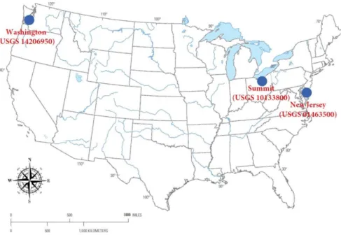
Three stations located in Washington County (USGS 14206950), Summit County (USGS 10133800), and New Jersey (USGS 01463500) of the USA are considered as the case study (Figure3). The water quality data recorded at those three stations for the period January 2002 to December 2016 were extracted from the United States Geological Survey (USGS) website (USGS, 2017). In fact, data for several water quality monitoring stations are available on the USGS website that could be used for the development of model. Nevertheless, the data for all the water quality parameters are not available or not reliable for the selected duration at most of the stations. In addition, as can be observed from Figure3, the three selected stations are located at different regions which can allow us to examine the performance of the proposed models under different geographical and climatic conditions. Furthermore, Heddam and Kisi (2018) developed a model for the prediction of DO concentration at the same stations [51]. In order to carry out a rational comparison with the previous research findings, the proposed models are developed for the prediction of DO concentration at the same selected stations.

(9)

Water2018,10, 1124 9 of 21

available or not reliable for the selected duration at most of the stations. In addition, as can be observed from Figure 3, the three selected stations are located at different regions which can allow us to examine the performance of the proposed models under different geographical and climatic conditions. Furthermore, Heddam and Kisi (2018) developed a model for the prediction of DO concentration at the same stations [51]. In order to carry out a rational comparison with the previous research findings, the proposed models are developed for the prediction of DO concentration at the same selected stations.

Figure 3. The locations of the three case study sites in Washington (USGS 14206950), Summit (USGS 10133800), and New Jersey (USGS 01463500), USA.

The observed data were divided into three sets for the training (2002–2010), validation (2011– 2013), and testing (2014–2016) of the models at USGS 10133800 and USGS 01463500, while data for the period 2003–2010 was used for training at USGS 14206950 as data are available only from 2003 at this station. More details of the geographical information and historical data division for the training, validation, and testing of the model are given in Table 1. The water quality parameters including water temperature (WT), discharge (Q, cfs), pH (sd, unit), specific conductance (SC, µS/cm), and DO (mg/lit) are used in the present study. Table 2 shows the statistical information of the water quality parameters. The Pearson coefficient based on the following equation is used to measure the correlation of different parameters with DO:

(

)

(

)

(

)

, cov , x y x y X Y X Y E X Y X Y

μ

ρ

σ σ

 ₋ ₋    = = (19)

where cov is the covariance between quantitative X and Y; σX _andσY _{are the standard deviations} of X and Y, respectively; μx _andμy_{are the averages of}_X_and_Y_{, respectively; and}

E

_{is the} expectation value.

Figure 3.The locations of the three case study sites in Washington (USGS 14206950), Summit (USGS 10133800), and New Jersey (USGS 01463500), USA.

The observed data were divided into three sets for the training (2002–2010), validation (2011–2013), and testing (2014–2016) of the models at USGS 10133800 and USGS 01463500, while data for the period 2003–2010 was used for training at USGS 14206950 as data are available only from 2003 at this station. More details of the geographical information and historical data division for the training, validation, and testing of the model are given in Table1. The water quality parameters including water temperature (WT), discharge (Q, cfs), pH (sd, unit), specific conductance (SC,µS/cm), and DO (mg/lit) are used in the present study. Table2shows the statistical information of the water quality parameters. The Pearson coefficient based on the following equation is used to measure the correlation of different parameters with DO:

ρx,y= cov (X,Y) σXσY = E (X−µx) Y−µy σXσY (19) where cov is the covariance between quantitativeXandY;σX andσYare the standard deviations ofX

andY, respectively;µxandµyare the averages ofXandY, respectively; andEis the expectation value.

Table 1.Geographical information and division of historical data into the training, validation, and testing periods.

Description USGS 14206950 USGS 10133800 USGS 01463500

Latitude 45◦2401300 40◦4503500 40◦1301800 Longitude 122◦4501300 111◦3304800 74◦4604100 Begin Date 01/01/2003 01/01/2002 01/01/2002 End Date 31/12/2016 31/12/2016 31/12/2016 Training period 2003–2010 2002–2010 2002–2010 Validation period 2011–2013 2011–2013 2011–2013 Test period 2014–2016 2014–2016 2014–2016

(10)

Table 2. The statistical properties of the water quality variables used in this study at the three investigated monitoring stations.

Station Data Unit Xmean Xmax Xmin Sx Cv

USGS 14206950 WT ◦C 12.619 24.800 0.100 5.190 0.411 pH - 7.281 7.900 6.500 0.177 0.024 SC µS/cm 200.769 461.00 61.000 54.889 0.273 Q cfs 47.368 1410.000 0.990 87.995 1.858 DO mg/lit 12.619 24.800 0.100 5.190 0.411 USGS 10133800 WT ◦C 9.179 22.00 0.300 6.148 0.670 pH - 7.961 8.600 6.800 0.233 0.029 SC µS/cm 1224.585 3530.00 453.000 313.211 0.256 Q cfs 32.927 371.000 2.20 40.722 1.238 DO mg/lit 9.076 12.80 4.70 1.369 0.151 USGS 01463500 WT ◦C 13.344 30.300 −0.200 8.984 0.673 pH 7.893 9.800 6.300 0.492 0.062 SC µS/cm 193.572 448.00 74.00 43.264 0.223 Q cfs 13940.65 230000 2370. 14626.481 1.049 DO mg/lit 11.056 16.900 5.40 2.263 0.205

Note: Xmean: mean; Xmax: maximum; Xmin: minimum; Sx: standard deviation; Cv: coefficient of variation; cfs: cubic feet per second;µS/cm: micro Siemens per centimeter, mg/lit: milligrams per liter.

The studied variables should be normalized to have the same scale so that the mean equals 0 and the standard deviation equals 1. The Z score method is used for this issue [75]:

xn,ik=

xi,k−mk

Sdk

(20) wherexn,ikis the normalized parameter,mkis the mean value, andSdkis the standard deviation.

The following indices are used for the evaluation of the different models:

R=       1 N∑(Oi−Om)(Xi−Xm) s 1 N N ∑ i=1 (Oi−Om) s 1 N N ∑ i=1 (Xi−Xm)       (21) RMSE= v u u t1 N N

∑

i=1 (Oi−Xi)2 (22) MAE= 1 N N

∑

i=1 |Oi−Xi| (23)

whereOi: observed DO,Om: average of observed DO,Xi: predicated value of DO, Xm: average

predicated value of DO,N: number of datapoints,MAE: mean absolute error,RMSE: root-mean-square error, andR: determination of coefficient [76,77].

4. Results and Discussion

4.1. The Correlations between DO and Other Water Quality Parameters

Table3presents the correlation coefficient between DO and other water quality parameters. The highest correlation of DO is found with WT followed by SC at all three monitoring stations. The least value of correlation coefficient at all three stations was found for pH. Different input combinations were constructed based on the correlation analysis presented in Table3. Table4shows

(11)

Water2018,10, 1124 11 of 21

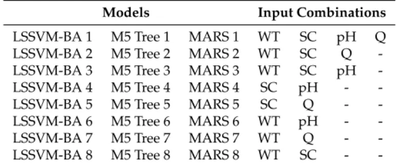
different input combinations based on four water quality parameters, namely, WT, SC, Q, and pH. Two combinations are considered without WT to determine the effectiveness of other parameters in the absence of WT in predicting DO. Besides this, two combinations of three variables and one combination of four variables were suggested for investigating the optimum input variables for prediction of DO.

Table 3.The correlation coefficients between DO and other water quality parameters.

Parameter DO Q SC pH WT USGS 14206950 DO (mg/lit) 1 - - - -Q (cfs) 0.196 1 - - -SC (µS/cm) −0.678 −0.612 1 - -pH 0.112 −0.561 0.378 1 -WT (◦C) −0.981 −0.224 0.614 −0.024 1 USGS 10133800 DO (mg/lit) 1 - - - -Q (cfs) 0.187 1 - - -SC (µS/cm) 0.312 −0.525 1 - -pH 0.111 0.311 −0.374 1 -WT (◦C) −0.944 −0.054 −0.444 −0.212 1 USGS 01463500 DO (mg/lit) 1 - - - -Q (cfs) 0.223 1 - - -SC (µS/cm) −0.281 −0.565 1 - -pH 0.109 −0.320 −0.606 1 -WT (◦C) −0.912 −0.264 0.238 0.194 1

Table 4.The input combinations used for the development of prediction models.

Models Input Combinations

LSSVM-BA 1 M5 Tree 1 MARS 1 WT SC pH Q

LSSVM-BA 2 M5 Tree 2 MARS 2 WT SC Q

-LSSVM-BA 3 M5 Tree 3 MARS 3 WT SC pH

-LSSVM-BA 4 M5 Tree 4 MARS 4 SC pH -

-LSSVM-BA 5 M5 Tree 5 MARS 5 SC Q -

-LSSVM-BA 6 M5 Tree 6 MARS 6 WT pH -

-LSSVM-BA 7 M5 Tree 7 MARS 7 WT Q -

-LSSVM-BA 8 M5 Tree 8 MARS 8 WT SC -

-4.2. Sensitivity Analysis of Bat Algorithm Parameters

The root-mean-square error is considered as the objective function for the evaluation of results. The evolutionary nature-inspired algorithms have parameters with random natures and, thus, sensitivity analysis is necessary to determine the accurate values of these parameters. The parameter values are varied, and the sensitivity of the parameters is computed against the variations of the objective function. When the RMSE is selected as the objective function, the aim of the problem is to minimize the objective function to compute the best value of different parameters. The first combination of inputs is selected for the explanation of the sensitivity analysis. The results of the sensitivity analysis using other input combinations are not provided in order to avoid repetition.

An important point to report here is that there are some parameters such as the maximum frequency, minimum frequency, and loudness that drive bats in the optimized path. The decision variables are bats’ positions or unknown parameters of LSSVM. The parameters such as maximum frequency, minimum frequency, or loudness are mathematical or physical parameters that lead the

(12)

bats or solution to the best position or best solution. Therefore, these parameters adjust the sounds and the bats are led to the best position for finding the food (or the best solution).

Table5shows the results of sensitivity analysis of the bat algorithm at all the three investigated water quality monitoring stations. The population size for the bat algorithm was varied from 20 to 80. The objective function was found to have the least value (0.882 mg/lit) for the population size 60 at the USGS 14206950 station. The minimum frequency was varied from 0.1 to 0.4 and the best value was obtained as 0.2. The maximum frequency was varied between 0.30 and 0.90 and the least value (0.882 mg/lit) of the objective function was found for 0.7 Hz. The least value of the objective function was found for the maximum loudness of 5 dB. The maximum number for the basis function for the MARS model at all the stations is considered as 130. The backward stage based on the condition of the problem and inputs are considered for tree pruning in order to have the maximum pruning. The M5 Tree model does not require any user-defined parameters. The process continues for the M5 Tree model until the SDR value is smaller than the expected value. All the methods have the same complexity, in terms of computation time.

Table 5.The sensitivity of the parameters of the bat algorithm at the three investigated water quality monitoring stations. Population Size Objective Function (mg/lit) Maximum Frequency Objective Function (mg/lit) Minimum Frequency Objective Function (mg/lit) Maximum Loudness Objective Function (mg/lit) USGS 4206950 20 0.944 0.30 0.934 0.10 0.921 3 0.910 40 0.921 0.50 0.921 0.20 0.882 5 0.882 60 0.882 0.70 0.882 0.30 0.914 7 0.889 80 0.912 0.90 0.914 0.40 0.955 9 0.901 USGS 0133800 20 0.956 0.30 0.921 0.10 0.931 3 0.954 40 0.916 0.50 0.899 0.20 0.916 5 0.892 60 0.892 0.70 0.892 0.30 0.892 7 0.912 80 0.901 0.90 0.912 0.40 0.912 9 0.916 USGS01463500 20 0.935 0.30 0.925 0.10 0.929 3 0.934 40 0.919 0.50 0.911 0.20 0.912 5 0.895 60 0.895 0.70 0.895 0.30 0.895 7 0.912 80 0.901 0.90 0.902 0.40 0.910 9 0.921

4.3. Modeling River Dissolved Oxygen Concentration

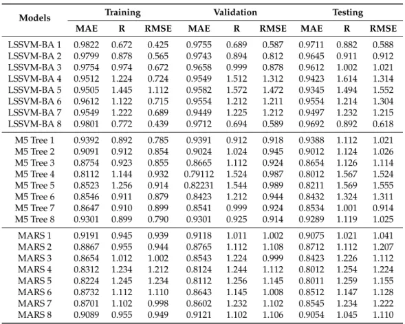
Table 6 shows the performance of the different predictive models with different input combinations over the training, validation, and testing phases at USGS 14206950 station. The least values of the absolute error are found for the first input combination for all the predictive models (LSSVM-BA, M5 Tree, and MARS). This indicates that it is possible to supply more information to the predictive model through incorporation of all the predictors. The worst performance is noticed for LSSVM-BA 4 and LSSVM-BA 5 models during the training phase. Better performance of LSSVM-BA compared with M5 Tree and MARS models is found consistently for all the input combinations.

(13)

Water2018,10, 1124 13 of 21

Table 6. The performance indicators of the predictive models during training/validation/testing phases at USGS 14206950.

Models Training Validation Testing

MAE R RMSE MAE R RMSE MAE R RMSE

LSSVM-BA 1 0.9822 0.672 0.425 0.9755 0.689 0.587 0.9711 0.882 0.588 LSSVM-BA 2 0.9799 0.878 0.565 0.9743 0.894 0.812 0.9645 0.911 0.912 LSSVM-BA 3 0.9754 0.974 0.672 0.9658 0.999 0.878 0.9612 1.002 1.021 LSSVM-BA 4 0.9512 1.224 0.724 0.9549 1.512 1.312 0.9423 1.614 1.314 LSSVM-BA 5 0.9505 1.445 1.112 0.9582 1.572 1.472 0.9345 1.494 1.552 LSSVM-BA 6 0.9612 1.122 0.715 0.9554 1.212 1.211 0.9554 1.214 1.304 LSSVM-BA 7 0.9549 1.222 0.689 0.9449 1.225 1.212 0.9497 1.232 1.215 LSSVM-BA 8 0.9801 0.772 0.439 0.9712 0.694 0.589 0.9692 0.892 0.618 M5 Tree 1 0.9392 0.892 0.785 0.9391 0.912 0.918 0.9388 1.112 1.021 M5 Tree 2 0.9091 0.912 0.854 0.9024 1.024 0.945 0.9012 1.124 1.026 M5 Tree 3 0.8754 0.923 0.855 0.8665 1.112 0.924 0.8654 1.126 1.114 M5 Tree 4 0.8112 1.144 0.932 0.79112 1.524 0.987 0.8012 1.567 1.524 M5 Tree 5 0.8523 1.256 0.914 0.82231 1.544 0.989 0.8211 1.569 1.555 M5 Tree 6 0.8546 0.911 0.879 0.8423 1.212 0.944 0.8432 1.324 1.311 M5 Tree 7 0.8647 0.910 0.899 0.8541 0.999 0.924 0.8534 1.001 0.914 M5 Tree 8 0.9301 0.899 0.790 0.9301 0.925 0.914 0.9289 1.119 1.025 MARS 1 0.9191 0.945 0.939 0.9118 1.011 1.002 0.9075 1.021 1.041 MARS 2 0.8867 0.955 0.944 0.8765 1.112 1.108 0.8712 1.112 1.207 MARS 3 0.8654 1.012 1.002 0.8543 1.224 0.999 0.8423 1.226 1.112 MARS 4 0.8312 1.234 1.212 0.8124 1.244 1.112 0.8012 1.254 1.224 MARS 5 0.8224 1.245 1.234 0.8112 1.256 1.145 0.8011 1.259 1.155 MARS 6 0.8732 1.112 1.110 0.8643 1.145 1.008 0.8512 1.147 1.128 MARS 7 0.8701 1.102 0.998 0.8602 1.232 1.102 0.8545 1.234 1.222 MARS 8 0.9089 0.955 0.949 0.9121 1.102 1.106 0.9054 1.045 1.110

The least values of RMSE and MAE are found for the LSSVM-BA 1 during training (0.672 and 0.425 mg/lit), validation (0.689 and 0.912 mg/lit), and testing (0.882 and 0.588 mg/lit). The first input combination is also found to be best in terms of correlation. The results in Table6demonstrate the significance of WT in the prediction of DO. The LSSVM-BA 1 showed enhancement over M5 Tree 1 and MARS 1 by 20% and 42% in terms of RMSE and 13% and 45% in terms of MAE, respectively, during the testing phase. This clearly indicates the capability of the integrative model (LSSVM-BA) and the potential of the nature-inspired algorithm for tuning LSSVM parameters.

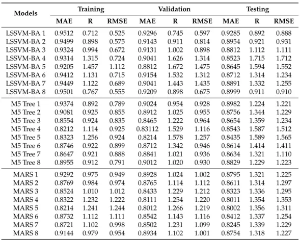
Table7shows the performance of the LSSVM-BA, M5 Tree, and MARS models in prediction of DO at USGS 10133800 station during all the modeling phases. From Table7, it is clear that LSSVM-BA performed better compared with the M5 tree and MARS. This can be elaborated through the results of RMSE and MAE. The least values of RMSE and MAE are achieved for the LSSVM-BA 1 during model training (0.712 and 0.525 mg/lit), validation (0.745 and 0.597 mg/lit), and testing (0.892 and 0.888 mg/lit). The performance of the LSSVM-BA model is evaluated against the best results obtained using M5 Tree and MARS models. The prediction accuracy of LSSVM-BA model is found to improve in term of RMSE and MAE by 27% and 27.4%, and by 32% and 27.5% for M5 Tree and MARS models, respectively. The eighth input combination (LSSVM-BA 8), i.e., with two inputs, WT and SC, is found to have a performance close to that of the best input combination (LSSVM-BA 1). This indicates an alternative in the case of limited data. In such a condition, WT and SC only can be used for the development of a DO prediction model.

(14)

Table 7. The performance of the predictive models during training/validation/testing at USGS 10133800 station.

It is worthwhile to validate the current research with the literature. The comparison of the results with those obtained in other studies showed that the LSSVM-BA can decrease RMSE in model prediction by about 5–11% compared with classical SVM [36]. There are some critical observations of Table7. For example, all the three predictive models behave differently for the 5th input combination. The reason for this is the uncertainty and low correlation of DO with the input. With respect to this, a Bayesian method is considered for measuring the uncertainty of model parameters and their effect on DO [57]. The results showed that the pH has the least weight or most uncertainty among all the parameters. Thus, incorporation of more parameters does not guarantee the successful performance of the models.

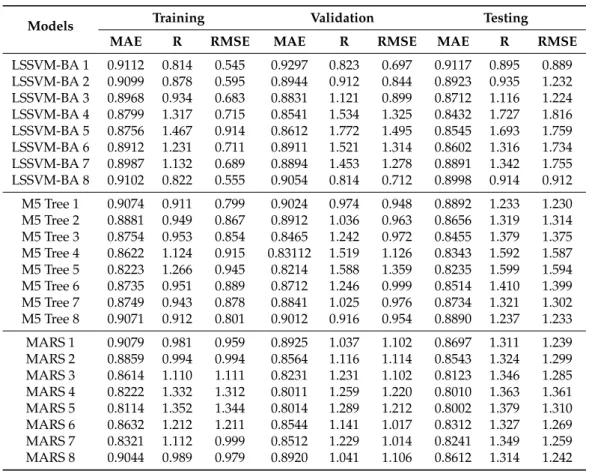
Table8shows the performance of LSSVM-BA, M5 Tree, and MARS models during different modeling phases at USGS 01463500 station. Based on the statistical results presented in Table 8, the LSSVM-BA accomplishes the best results over the other models. The best results in term of RMSE and MAE are achieved for the first input combination and LSSVM-BA model during all the modeling phases. The best RMSE and MAE are found to be 0.814 and 0.545 mg/lit during training, 0.823 and 0.697 mg/lit during validation, and 0.895 and 0.889 mg/lit during testing. The evaluation of the proposed LSSVM-BA model compared with the best results obtained using the M5 Tree and MARS models during the testing phase revealed the better prediction accuracy of LSSVM-BA in terms of RMSE and MAE by 27.4% and 27.7% and 31.7% and 28.2% over the M5 Tree and MARS models.

(15)

Water2018,10, 1124 15 of 21

Table 8. The performance of the predictive models during training/validation/testing at USGS 01463500 station.

In general, the results of the three investigated stations are found to collaborate well with previous findings. Heddam and Kisi et al. (2017) showed that the regression methods without accurate estimation of some unknown parameters in their structure have a weaker performance compared with other AI methods such as ANN. Hence, the regression methods can be improved by the optimization of model parameters [77–79]. Other studies in the literature have also showed that the application of regression models with heuristic methods can improve model performance [80].

The performance of the models was also investigated using a scatter plot of observed and simulated values of DO concentration. Figures4–6shows the scatter plots for all the three stations during three modeling phases (i.e., training, validation, and testing). In general, the proposed integrative model displays a better correlation performance compared with the M5 Tree and MARS models. A closer examination revealed that the prediction was excellent for the whole range of DO values (0.10–24.8 mg/lit) at USGS 14206950 station. Relatively lower performance for the DO concentrations between 6.5–7.9 and 9.7–11.18 mg/lit is observed at USGS 10133800 station, particularly during the testing phase. This can be justified through the lack of the input attribute information at this particular station. Besides this, the concentration of dissolved oxygen may be affected by other environmental influences at this station. Relatively better performance in prediction of all values of DO concentration (5.4–16.9 mg/lit) is observed at USGS 01463500 station.

(16)

Figure 4. Scatter plot of observed and simulated DO concentration by three predictive models during model training, validation, and testing at USGS 14206950.

5. Conclusions

Water quality is a major concern in water resource management. Among several water quality variables, DO is the main concern in term of aquatic environment and ecology. The magnitude of DO relies on several other water quality variables and interactions among the variables, and, thus, the modeling of DO is an interesting but complex topic in environmental science. A novel modeling strategy based on integration of a nature-inspired algorithm with LSSVM was proposed in this study for the prediction of DO at three river water quality monitoring stations located in the USA. The results were compared with those obtained using MT5 and MARS models. The overall findings of the study are as follows:

• The performance of LSSVM-BA 1 was found to be best among all the models based on higher correlation (see Figure 4) and lower RMSE and MAE compared with the other models at all Figure 4.Scatter plot of observed and simulated DO concentration by three predictive models during model training, validation, and testing at USGS 14206950.

5. Conclusions

• The performance of LSSVM-BA 1 was found to be best among all the models based on higher correlation (see Figure 4) and lower RMSE and MAE compared with the other models at all

Figure 5.Scatter plot of observed and simulated DO concentration by three predictive models during model training, validation, and testing at USGS 10133800.

5. Conclusions

• The performance of LSSVM-BA 1 was found to be best among all the models based on higher correlation (see Figure 4) and lower RMSE and MAE compared with the other models at all

Figure 6.Scatter plot of observed and simulated DO concentration by three predictive models during model training, validation, and testing at USGS 01463500.

5. Conclusions

Water quality is a major concern in water resource management. Among several water quality variables, DO is the main concern in term of aquatic environment and ecology. The magnitude of DO relies on several other water quality variables and interactions among the variables, and, thus, the modeling of DO is an interesting but complex topic in environmental science. A novel modeling strategy based on integration of a nature-inspired algorithm with LSSVM was proposed in this study for the prediction of DO at three river water quality monitoring stations located in the USA. The results

(17)

Water2018,10, 1124 17 of 21

were compared with those obtained using MT5 and MARS models. The overall findings of the study are as follows:

• The performance of LSSVM-BA 1 was found to be best among all the models based on higher correlation (see Figure4) and lower RMSE and MAE compared with the other models at all three stations (see Tables6–8). For instance, LSSVM-BA 1 for the USGS 14206950 station showed better accuracy by 3.1%, 11%, 45%, 40%, 27%, 28%, and 29% than the LSSVM-BA 2, LSSVM-BA 3, LSSVM-BA 4, LSSVM-BA 5, LSSVM-BA 6, LSSVM-BA 7, and LSSVM-BA 8 models.

• The MARS 1 and M5 Tree 1 models showed the lowest RMSE and MAE among all the MARS and M5 Tree models at all three stations during all three modeling phases (training, validation, and testing).

• The fourth and the fifth input combinations (without the WT parameter) showed the worst performance among all the input combinations at all the three stations at all the three modeling phases, which indicates the importance of WT in prediction of DO.

• All three predictive models (LSSVM, MARS, and M5 Tree) showed relatively better performance when only WT and SC were used as input at two stations, namely, USGS 10133800 and USGS 01463500, which indicates that WT and SC can be used for reasonable prediction of DO when other water quality data are not available.

Overall, the results showed better performance of the LSSVM-BA model compared with other models. As further research, the nature-inspired algorithms used in the current research can be considered for the improvement of other methods such as ANN and ANFIS. Furthermore, the performance of LSSVM-BA against those improved models can be evaluated to find the best model for river DO prediction. In addition, the improved models can be used for the prediction of daily or hourly DO concentration in shallow water bodies to show their efficacy in prediction of DO concentration under different environmental conditions.

Author Contributions: Conceptualization, Ahmed El-Shafie; Methodology, Mohammad Ehteram; Software, Mohammad Ehteram; Validation, Zaher Mundher Yaseen and Ahmad Sharafati; Formal Analysis, Nadhir Al-Ansari; Investigation, Nadhir Al-Ansari; Data Curation, Mohammad Ehteram; Writing-Original Draft Preparation, Mohammad Ehteram and Ahmad Sharafati; Writing-Review & Editing, Shamsuddin Shahid; Visualization, Zaher Mundher Yaseen; Supervision, Ahmed El-Shafie.

Funding:The research was funded by the Universiti Teknologi Malaysia GUP grant No. 19H44.

Acknowledgments:The authors thank the reviewers and editors for their significant comments to improve the paper context.

Conflicts of Interest:The authors declare no conflict of interest. References

1. Šiljić Tomić, A.; Antanasijević, D.; Ristić, M.; Perić-Grujić, A.; Pocajt, V. A linear and non-linear polynomial neural network modeling of dissolved oxygen content in surface water: Inter- and extrapolation performance with inputs’ significance analysis.Sci. Total Environ.2018,610–611, 1038–1046. [CrossRef] [PubMed] 2. Post, C.J.; Cope, M.P.; Gerard, P.D.; Masto, N.M.; Vine, J.R.; Stiglitz, R.Y.; Hallstrom, J.O.; Newman, J.C.;

Mikhailova, E.A. Monitoring spatial and temporal variation of dissolved oxygen and water temperature in the Savannah River using a sensor network.Environ. Monit. Assess.2018,190, 272. [CrossRef] [PubMed] 3. Boyd, C.E.; Torrans, E.L.; Tucker, C.S. Dissolved Oxygen and Aeration in Ictalurid Catfish Aquaculture.

J. World Aquac. Soc.2018,49, 7–70. [CrossRef]

4. Reeder, W.J.; Quick, A.M.; Farrell, T.B.; Benner, S.G.; Feris, K.P.; Tonina, D. Spatial and Temporal Dynamics of Dissolved Oxygen Concentrations and Bioactivity in the Hyporheic Zone.Water Resour. Res.2018. [CrossRef] 5. Khan, U.T.; Valeo, C. Comparing a Bayesian and fuzzy number approach to uncertainty quantification in

short-term dissolved oxygen prediction.J. Environ. Inform.2017,30, 1–16. [CrossRef]

6. He, J.; Chu, A.; Ryan, M.C.; Valeo, C.; Zaitlin, B. Abiotic influences on dissolved oxygen in a riverine environment.Ecol. Eng.2011,37, 1804–1814. [CrossRef]

(18)

7. Chapra, S.C.; Pelletier, G.J.; Tao, H.QUAL2K: A Modeling Framework for Simulating River and Stream Water Quality: Documentation and Users Manual; Civil and Environmental Engineering Dept., Tufts University: Medford, MA, USA, 2003.

8. Wool, T.A.; Ambrose, R.B.; Martin, J.L.; Comer, E.A.; Tech, T. Water quality analysis simulation program (WASP). 2006. Available online: https://www.epa.gov/ceam/water-quality-analysis-simulation-program-wasp(accessed on 22 August 2018).

9. Ahmed, A.A.M. Prediction of dissolved oxygen in Surma River by biochemical oxygen demand and chemical oxygen demand using the artificial neural networks (ANNs).J. King Saud Univ.—Eng. Sci.2017,29, 151–158. [CrossRef]

10. Cox, B.A. A review of dissolved oxygen modelling techniques for lowland rivers.Sci. Total Environ.2003, 314, 303–334. [CrossRef]

11. Zounemat-Kermani, M.; Scholz, M. Modeling of Dissolved Oxygen Applying Stepwise Regression and a Template-Based Fuzzy Logic System.J. Environ. Eng.2014. [CrossRef]

12. Li, X.; Sha, J.; Wang, Z. A comparative study of multiple linear regression, artificial neural network and support vector machine for the prediction of dissolved oxygen.Hydrol. Res.2017,48, 1214–1225. [CrossRef] 13. Kuok, K.K.; Kueh, S.M.; Chiu, P.C. Bat optimisation neural networks for rainfall forecasting: Case study for

Kuching city.J. Water Clim. Chang.2018. [CrossRef]

14. Sulaiman, J.; Wahab, S.H. Heavy Rainfall Forecasting Model Using Artificial Neural Network for Flood Prone Area. InIT Convergence and Security 2017; Springer: Singapore, 2018; pp. 68–76.

15. Shank, D.B.; Hoogenboom, G.; McClendon, R.W. Dewpoint temperature prediction using artificial neural networks.J. Appl. Meteorol. Climatol.2008,47, 1757–1769. [CrossRef]

16. Radhika, Y.; Shashi, M. Atmospheric temperature prediction using support vector machines.Int. J. Comput. Theory Eng.2009,1, 55. [CrossRef]

17. Pal, M.; Deswal, S. M5 model tree based modelling of reference evapotranspiration.Hydrol. Process.2009,23, 1437–1443. [CrossRef]

18. Granata, F.; Gargano, R.; De Marinis, G. Support Vector Regression for Rainfall-Runoff Modeling in Urban Drainage: A Comparison with the EPA’s Storm Water Management Model.Water2016,8, 69. [CrossRef] 19. Granata, F.; Papirio, S.; Esposito, G.; Gargano, R.; De Marinis, G. Machine learning algorithms for the

forecasting of wastewater quality indicators.Water2017,9, 2. [CrossRef]

20. Liu, Y.; Sang, Y.-F.; Li, X.; Hu, J.; Liang, K. Long-Term Streamflow Forecasting Based on Relevance Vector Machine Model.Water2016,9, 9. [CrossRef]

21. Candelieri, A. Clustering and support vector regression for water demand forecasting and anomaly detection. Water2017,9, 224. [CrossRef]

22. Ji, X.; Shang, X.; Dahlgren, R.A.; Zhang, M. Prediction of dissolved oxygen concentration in hypoxic river systems using support vector machine: A case study of Wen-Rui Tang River, China.Environ. Sci. Pollut. Res.

2017,24, 16062–16076. [CrossRef] [PubMed]

23. Huang, J.; Yin, H.; Chapra, S.C.; Zhou, Q. Modelling dissolved oxygen depression in an urban river in China. Water2017,9, 520. [CrossRef]

24. Heddam, S.; Kisi, O. Extreme learning machines: A new approach for modeling dissolved oxygen (DO) concentration with and without water quality variables as predictors. Environ. Sci. Pollut. Res.2017,24, 16702–16724. [CrossRef] [PubMed]

25. Keshtegar, B.; Heddam, S. Modeling daily dissolved oxygen concentration using modified response surface method and artificial neural network: A comparative study.Neural Comput. Appl.2017, 1–12. [CrossRef] 26. Liu, S.; Yan, M.; Tai, H.; Xu, L.; Li, D. Prediction of dissolved oxygen content in aquaculture of Hyriopsis

Cumingii using Elman neural network. 2011. Available online:https://link.springer.com/chapter/10.1007/ 978-3-642-27275-2_57(accessed on 22 August 2018).

27. Akkoyunlu, A.; Altun, H.; Cigizoglu, H.K. Depth-integrated estimation of dissolved oxygen in a lake. J. Environ. Eng.2011,137, 961–967. [CrossRef]

28. Ay, M.; Kisi, O. Modeling of dissolved oxygen concentration using different neural network techniques in Foundation Creek, El Paso County, Colorado.J. Environ. Eng.2011,138, 654–662. [CrossRef]

29. Bayram, A.; Uzlu, E.; Kankal, M.; Dede, T. Modeling stream dissolved oxygen concentration using teaching–learning based optimization algorithm.Environ. Earth Sci.2015,73, 6565–6576. [CrossRef]

(19)

Water2018,10, 1124 19 of 21

30. Chen, Y.; Xu, J.; Yu, H.; Zhen, Z.; Li, D. Three-dimensional short-term prediction model of dissolved oxygen content based on pso-bpann algorithm coupled with kriging interpolation.Math. Probl. Eng.2016,2016. [CrossRef]

31. Diamantopoulou, M.J.; Antonopoulos, V.Z.; Papamichail, D.M. Cascade correlation artificial neural networks for estimating missing monthly values of water quality parameters in rivers.Water Resour. Manag.2007,21, 649–662. [CrossRef]

32. Heddam, S. Use of optimally pruned extreme learning machine (OP-ELM) in forecasting dissolved oxygen concentration (DO) several hours in advance: A case study from the Klamath River, Oregon, USA. Environ. Process.2016,3, 909–937. [CrossRef]

33. Heddam, S. Generalized regression neural network (GRNN)-based approach for colored dissolved organic matter (CDOM) retrieval: Case study of Connecticut River at Middle Haddam Station, USA.Environ. Monit. Assess.2014,186, 7837–7848. [CrossRef] [PubMed]

34. Liu, S.; Xu, L.; Li, D.; Li, Q.; Jiang, Y.; Tai, H.; Zeng, L. Prediction of dissolved oxygen content in river crab culture based on least squares support vector regression optimized by improved particle swarm optimization. Comput. Electron. Agric.2013,95, 82–91. [CrossRef]

35. Liu, S.; Xu, L.; Jiang, Y.; Li, D.; Chen, Y.; Li, Z. A hybrid WA–CPSO-LSSVR model for dissolved oxygen content prediction in crab culture.Eng. Appl. Artif. Intell.2014,29, 114–124. [CrossRef]

36. Mohammadpour, R.; Shaharuddin, S.; Chang, C.K.; Zakaria, N.A.; Ghani, A.A.; Chan, N.W. Prediction of water quality index in constructed wetlands using support vector machine.Environ. Sci. Pollut. Res.2014, 6208–6219. [CrossRef] [PubMed]

37. Jadhav, M.S.; Khare, K.C.; Warke, A.S. Water Quality Prediction of Gangapur Reservoir (India) Using LS-SVM and Genetic Programming.Lakes Reserv. Res. Manag.2015,20, 275–284. [CrossRef]

38. Ranković, V.; Radulović, J.; Radojević, I.; Ostojić, A.; ˇComić, L. Prediction of dissolved oxygen in reservoirs using adaptive network-based fuzzy inference system.J. Hydroinform.2012,14, 167–179. [CrossRef] 39. Heddam, S. Modeling hourly dissolved oxygen concentration (DO) using two different adaptive neuro-fuzzy

inference systems (ANFIS): A comparative study.Environ. Monit. Assess. 2014,186, 597–619. [CrossRef] [PubMed]

40. Heddam, S. Modelling hourly dissolved oxygen concentration (DO) using dynamic evolving neural-fuzzy inference system (DENFIS)-based approach: Case study of Klamath River at Miller Island Boat Ramp, OR, USA.Environ. Sci. Pollut. Res.2014,21, 9212–9227. [CrossRef] [PubMed]

41. Ay, M.; Ki¸si, Ö. Estimation of dissolved oxygen by using neural networks and neuro fuzzy computing techniques.KSCE J. Civ. Eng.2017,21, 1631–1639. [CrossRef]

42. Kisi, O.; Akbari, N.; Sanatipour, M.; Hashemi, A.; Teimourzadeh, K.; Shiri, J. Modeling of dissolved oxygen in river water using artificial intelligence techniques.J. Environ. Inform.2013,22, 92–101. [CrossRef] 43. Nemati, S.; Fazelifard, M.H.; Terzi, Ö.; Ghorbani, M.A. Estimation of dissolved oxygen using data-driven

techniques in the Tai Po River, Hong Kong.Environ. Earth Sci.2015,74, 4065–4073. [CrossRef]

44. Khani, S.; Rajaee, T. Modeling of Dissolved Oxygen Concentration and Its Hysteresis Behavior in Rivers Using Wavelet Transform-Based Hybrid Models.CLEAN—Soil Air Water2017,45. [CrossRef]

45. Mehdipour, V.; Memarianfard, M.; Homayounfar, F. Application of gene expression programming to water dissolved oxygen concentration prediction.Int. J. Hum. Cap. Urban. Manag.2017,2, 39–48. [CrossRef] 46. Singh, K.P.; Basant, N.; Gupta, S. Support vector machines in water quality management.Anal. Chim. Acta

2011,703, 152–162. [CrossRef] [PubMed]

47. Tan, G.; Yan, J.; Gao, C.; Yang, S. Prediction of water quality time series data based on least squares support vector machine.Procedia Eng.2012,31, 1194–1199. [CrossRef]

48. Granata, F.; De Marinis, G. Machine learning methods for wastewater hydraulics.Flow Meas. Instrum.2017, 57, 1–9. [CrossRef]

49. Malek, S.; Mosleh, M.; Syed, S.M. Dissolved oxygen prediction using support vector machine.Int. J. Bioeng. Life Sci.2014,8, 46–50.

50. Yu, H.; Chen, Y.; Hassan, S.; Li, D. Dissolved oxygen content prediction in crab culture using a hybrid intelligent method.Sci. Rep.2016. [CrossRef] [PubMed]

51. Heddam, S.; Kisi, O. Modelling daily dissolved oxygen concentration using least square support vector machine, multivariate adaptive regression splines and M5 model tree.J. Hydrol.2018. [CrossRef]