A matrix Method for Interval Hermite Curve Segmentation

(1)

International Journal of Video&Image Processing and Network Security IJVIPNS-IJENS Vol:15 No:03 7

153903-8484-IJVIPNS-IJENS © June 2015 IJENS

A matrix Method for Interval Hermite Curve

Segmentation

O. Ismail, Senior Member, IEEE

Abstract— Since the use of matrix forms (largely promoted in CAD/CAM) turns out to be both convenient and practical in representing parametric curves and surfaces. Furthermore, this implementation can be made extremely fast if appropriate matrix facilities are available in either hardware or software. We can break a curve down into smaller segments by truncating or subdividing it. There are many reasons for doing this. For example, we may truncate to isolate and extract that part of a curve surviving a model modification process, or subdivide it to compute points for displaying it. To truncate, subdivide, or change the direction of parameterization of a curve ordinarily requires a mathematical operation called reparamelerization. Ideally, this operation produces a change in the parametric interval so that neither the shape nor the position of the curve is changed. This effect is often referred to

as shape invariance under parameterization and

reparamelerization. This concept has been applied on interval Hermite curves. An algorithmic method for interval Hermite curve segmentation in matrix form is presented in this paper. To split the interval Hermite curve defined over the range

[ ]at a point defined by means that the first

and the second interval segments are to be defined over the ranges [ ] and [ ] , respectively. The four fixed Kharitonov's polynomials (four fixed Hermite curves) associated with the original interval Hermite curve are obtained. The proposed algorithm is applied to the four fixed Kharitonov's polynomials (four fixed Hermite curves) in order to obtain the fixed control points for the first and second fixed segments, respectively. Finally the interval control points for the first and second interval segments of the given interval Hermite curve are found from fixed control points for the four fixed Kharitonov's polynomials (four fixed Hermite curves) of the first and second fixed segments. A numerical example is included in order to demonstrate the effectiveness of the proposed method.

Index Term— Matrix representation, segmentation, interval Hermite curve, CAGD.

I. INTRODUCTION

Curve design is important in computer graphics, animation, and computer aided design. Unfortunately, curve design requires very involved mathematics even though many curve design concepts are intuitive. The curve is the most basic design element to determine shapes and silhouettes of industrial products and works for shape designers and it is inevitable for them to make it aesthetic and attractive to improve the total quality of the shape design. The Hermite curves and surfaces have been widely applied in many CAD/CAM systems. They have become a standard tool in industry of geometric modeling because they provide a common mathematical form for analytical geometry and free-form curves and surfaces.

The author is with Department of Computer Engineering, Faculty of Electrical and Electronic Engineering, University of Aleppo, Aleppo, (e-mail:[email protected]).

Geometric modeling and computer graphics have been interesting and important subjects for many years from the point of view of scientists and engineers.

One of the main and useful applications of these concepts is the treatment of curves and surfaces in terms of control points, a tool extensively used in CAGD.

There are several kinds of polynomial curves in CAGD, e.g., Bezier [1], [2], [3], [4], [5] Said-Ball [6], Wang-Ball [7], [8], [9], B-spline curves [10] and DP curves [11], [12]. These curves have some common and different properties. All of them are defined in terms of the sum of product of their blending functions and control points. They are just different in their own basis polynomials. In order to compare these curves, we need to consider these properties. The common properties of these curves are control points, weights, and their number of degrees. Control points are the points that affect to the shape of the curve. Weights can be treated as the indicators to control how much each control point influences to the curve. Number of degree determines the maximum degree of polynomials. In different curves, these properties are not computed by the same method. To compare different kinds of curves we need to convert these curves into an intermediate form.

Parametric equations avoid many of the problems associated with nonparametric functions. They also best describe the way curves are drawn by a plotter or some computer graphics display screens. Parametric equations generate the sets of points defining most of the curves, surfaces. Parametric equations have many advantages over other forms of representation. Here are the most important ones: (1) They allow separation of variables and direct computation of point coordinates. (2) It is easy to express parametric equations as vectors. (3) Each variable is treated alike. (4) There are more degrees of freedom to control curve shape. (5) Transformations may be performed directly on them. (6) They accommodate all slopes without computational breakdown. (7) Extension or contraction into higher or lower dimensions is direct and easy without affecting the initial representation. (8) The curves they define are inherently bounded when the parameter is constrained to a specified finite interval. (9) The same curve often can be represented by many different parameterizations. Conversely, a parameterization scheme is sometimes chosen because of its effect on curve shape.

(2)

International Journal of Video&Image Processing and Network Security IJVIPNS-IJENS Vol:15 No:03 8 Hermite curve is defined by its two end points and the

tangent vectors at those points. It interpolates all its control points and is fairly easy to subdivide. However, its lack of invariance under affine transformations can be troublesome if not accounted for. The cubic Hermite polynomial representation is the most interested representation, because this is the lowest degree capable of describing nonplanar curves. However, the Hermite form offers a practical alternative, allowing us to define a curve segment in terms of conditions at its endpoints, or boundaries. The Hermite basis functions first appear in the derivation of the geometric form from the algebraic form, each function is a curve over the domain of the parameter in the interval [ ]. Three important characteristics of these basis functions are: (1) Universality-they hold for all cubic Hermite curves. (2) Dimensional independence-they are identical for each of the three model-space coordinates, because they are dependent only on the parameter . (3) Separation of boundary condition effects-they allow the constituent boundary condition coefficients to be decoupled from each other. This means that we can selectively modify a single specific boundary condition to alter the shape of a curve without affecting the other boundary conditions. These functions blend the effects of the endpoints and tangent vectors to produce the intermediate point coordinate values over the domain of .

Matrix representation is very useful in computer aided geometric design, since the matrix is an important and basic tool in mathematics. Matrix formulas of Hermite curves and surfaces have the advantages of both simple computation of points on curves or surfaces and their derivatives and of easy analysis of the geometric properties of Hermite curves and surfaces.

Segmentation is a process of splitting a curve or a surface into a number of parts such that the composite curve or surface of all the segments is identical to the parent curve or surface. Segmentation is essentially a reparameterising transformation of a curve or a surface while keeping the degree of the curve or surface unchanged.

This paper is organized as follows. Section contains the basic results, whereas section shows a numerical example and the final section offers conclusions.

II. THEBASICRESULTS

Segmentation or curve splitting is defined as replacing one existing curve by one or more curve segments of the same curve type such that the shape of the composite curve is identical to that of the original curve. Segmentation is a very useful feature for CAD/CAM systems. Model cleanup for drafting purposes is an example where a curve might be divided into two at the line of sight of another. One of the resulting segments is then deleted. Another example is when a closed curve has to be split for modeling purposes. Mathematically, curve segmentation is a reparametrization or parameter transformation of the curve.

Polynomial curves such as Hermite curves, Bezier curves, and B-spline curves require a different parameter transformation. If the degree of the polynomial defining a curve is to be unchanged, which is the case in segmentation, the transformation must be linear.

Let us assume that the interval Hermite curve is defined over the range [ ] . To split the given interval curve at a point defined by means that the first and the second interval segments are to be defined over the range [ ] and [ ], respectively. A new parameter introduced for each interval segment such that its range is [ ]. The parameter transformation takes the form:

{ ( ₍ ) ₎ } ( )

In general, if the two interval endpoints [ ] and

[ ] and the first pairs of derivatives at the extreme points are known (a total of items), i.e.,

( ( )) ( ( )) ( ) , this will give [ ] [ ] [ ], they can be used to calculate an interval interpolating polynomial ( ) of degree , if we assume

, then the interval Hermite curve ( ) can be written in matrix form as follows:

( ) [ ] ( )

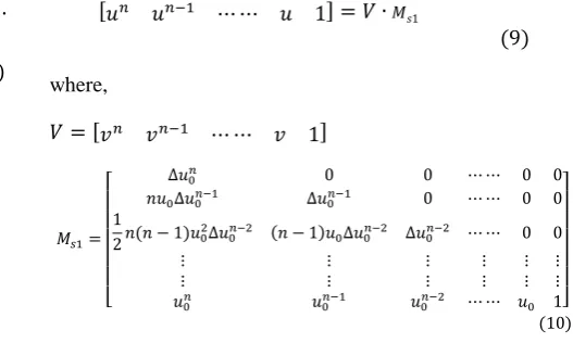
where,

[ _]

[[ ] [ ] [ ]]

( )

and is ( ) ( ) Hermite basis matrix.

The segmentation of an interval curve is needed when we want to utilize only a part of the interval curve and discard the remaining. When this utilized part is to be merged into the total model of the part being built, reparametrization is required as shown in Fig. 1.

The four fixed Kharitonov's polynomials (four fixed Hermite curves) [ ] in matrix form associated with the original interval Hermite curve are:

( ) [ ] ( )

( )

where,

[ ]

( )

and

( )

(3)

153903-8484-IJVIPNS-IJENS © June 2015 IJENS

( )

1 

v

0 

v

0 

v

0

u



m

u



1

u



1 

v

Fig. 1: Segmentation of interval Hermite Curve.

Now the segmentation of an interval Hermite curve can be converted into the following problem. For a given four fixed Kharitonov's polynomials (four fixed Hermite curves) associated with the original interval Hermite curve as in equation ( ), split the four fixed Kharitonov's polynomials (four fixed Hermite curves) at a point defined by , and find the fixed control points of the four fixed Kharitonov's polynomials (four fixed Hermite curves) for first and second fixed segments, finally the interval control points for the first and second interval segments of the given interval Hermite curve can be obtained from fixed control points for the four fixed Kharitonov's polynomials (four fixed Hermite curves) of the first and second fixed segments.

Hence, for first fixed segment,

{

{ ( ₍) ₎}

{₍ ( ₎ ) ( ₍) ₎( ) }

{₍ ( ₎ ) ( ₍) ₎ ( )₍ ₎( ) }

{₍₍ ( ₎) ₎} ∑ (₎

( )

}

( )

For second fixed segment,

{

{ ( ₍ ) ₎}

{₍ ( ₎) ( ₍) ₎( ) }

{₍ ( ₎) ( ₍) ₎ ( ) ₍ ( ₎) }

{₍₍ ( ₎) ₎} ∑ (₎

( )

}

( )

For first fixed segment, equation (7) can be written as follows:

[ _]

( )

where,

[ _]

[

( ) _{( )}

_] ( )

Therefore, for first fixed segment, the four fixed Kharitonov's polynomials (four fixed Hermite curves) in matrix form can be rewritten as:

( ) ( )

̃

( )

The modified geometry, or boundary conditions, vectors of the four fixed Kharitonov's polynomials (four fixed Hermite curves) first segment, are given by:

̃

( )

and

̃ [ ̃ ̃ ̃ ]

( )

The interval control points for the first interval segment of the given interval Hermite curve can be obtained from fixed control points of the four fixed Kharitonov's polynomials (four fixed Hermite curves) of the first fixed segments as:

[ ] [ ( ̃) ( ̃ )]

( ) ( )

( )

For second fixed segment, equation (8) can be written as follows:

[ _]

( )

where,

[ _]

[

( ) _{( )}

(4)

International Journal of Video&Image Processing and Network Security IJVIPNS-IJENS Vol:15 No:03 10 Therefore, for second fixed segment, the four fixed

Kharitonov's polynomials (four fixed Hermite curves) in matrix form can be rewritten as:

( ) ( )

̃

( )

The modified geometry, or boundary conditions, vectors of the four fixed Kharitonov's polynomials (four fixed Hermite curves) second segment, are given by:

̃

( )

and

̃ [ ̃ ̃ ̃ ]

( )

The interval control points for the second interval segment of the given interval Hermite curve can be obtained from the four fixed Kharitonov's polynomials (four fixed Hermite curves) of the second fixed segments as:

[ ] [ ( ̃) ( ̃)] ( )

( )

Interval Hermite curve segmentation can be done by the following steps:

Algorithm for the interval Hermite curve segmentation

1. Obtain the four fixed Kharitonov's polynomials (four fixed Hermite curves) associated with the original interval Hermite curve.

2. Split the four fixed Kharitonov's polynomials (four fixed Hermite curves) at a point defined by means that the first and the second fixed segments are to be defined over the range [ ] and [ ] , respectively.

3. The fixed control points of the four fixed Kharitonov's polynomials (four fixed Hermite curves) for first and second fixed segments can be obtained using equations (12) and (18), respectively.

4. The interval control points for the first and second

interval segments of the given interval Hermite curve can be obtained from fixed control points for the four fixed Kharitonov's polynomials (four fixed Hermite curves) of the first and second fixed segments using equations (14) and (20), respectively.

III.NUMERICALEXAMPLE

Consider the interval Hermite curve ( ), defined with interval endpoints:

[ ] ([ ] [ ]) [ ] ([ ] [ ])

for and interval tangent vectors at the two interval points are:

[ ] ([ ] [ ]) [ ] ([ ] [ ])

The problem is to divide the given interval Hermite curve into two interval segments at a point , and find the interval endpoints and interval slopes for each segment.

As explained in section , the four fixed Kharitonov's polynomials (four fixed Hermite curves) associated with the original interval Hermite are obtained, and the matrices

and for first fixed segment are found as follows:

[ ( )

( )

]

[

_]

The interval control endpoints for the first interval segment are obtained as:

[ ̃ ̃ ] ([ ] [ ]) [ ̃ ̃ ] ([ ] [ ])

with interval slopes at the interval endpoints,

[ ̃ ̃ ] ([ ] [ ]) [ ̃ ] ([ ] [ ])

Similarly, the matrix for second fixed segment is

found,

[

( )

( )( ) ( )

( )( )( ) ( ) ( )( )

( ) ( ) ]

The interval control endpoints for the second interval segment are obtained as:

[ ̃ ̃ ] ([ ] [ ]) [ ̃ ̃ ] ([ ] [ ])

with interval slopes at the interval endpoints,

[ ̃ ̃ ] ([ ] [ ]) [ ̃ ̃ ] ([ ] [ ])

IV.CONCLUSIONS

(5)

surfaces have the advantages of both simple computation of points on curves or surfaces and their derivatives and of easy analysis of the geometric properties of Hermite curves and surfaces. A simple matrix form for interval Hermite curve segmentation is presented in this paper. To split the interval Hermite curve defined over the range at a point defined by [ ] means that the first and the second interval segments are to be defined over the ranges and , respectively. The four fixed Kharitonov's polynomials (four fixed Hermite curves) associated with the original interval Hermite curve are obtained. The proposed algorithm is applied to the four fixed Kharitonov's polynomials (four fixed Hermite curves) in order to obtain the fixed control points for the first and second fixed segments, respectively. Finally the interval control points for the first and second interval segments of the given interval Hermite curve are found from fixed control points for the four fixed Kharitonov's polynomials (four fixed Hermite curves) of the first and second fixed segments. Splitting an interval Hermite curve implies creating two new interval curves, one that represents the

first interval half of

the original interval Hermite curve, and one that represents the second interval half. If the given interval Hermite curve is to be divided into more than two interval segments the proposed algorithm can be applied successively.

REFERENCES

[1] P. Bezier, "Deﬁnition Numerique Des Courbes et ̂ I", Automatisme, Vol. 11, pp. 625–632, 1966.

[2] P. Bezier, "Deﬁnition Numerique Des Courbes et ̂ II", Automatisme, Vol. 12, pp. 17–21, 1967.

[3] P. Bezier, Numerical control, Mathematics and Applications, New York: Wiley, 1972.

[4] G. Chang, “Matrix foundation of Bezier technique”, Comput. Aided Des. Vol. 14, No. 6, pp. 345-350, 1982.

[5] P. Bezier, The Mathematical Basis of the UNISURF CAD System, Butterworth, London, 1986.

[6] H. B. Said, "A generalized Ball curve and its recursive algorithm", ACM. Transaction on Graphics, Vol. 8, No. 4, pp. 360–371, 1989. [7] A. A. Ball, “CONSURF Part 1: Introduction to conic lofting tile”,

Computer Aided Design, Vol. 6, No. 4, pp. 243–249, 1974.

[8] A. A. Ball, ”CONSURF Part 2: Description of the algorithms”, Computer Aided Design, Vol. 7, No. 4, pp. 237–242, 1975.

[9] A. A. Ball, “CONSURF Part 3: How the program is used”, Computer Aided Design, Vol. 9, No. 1, pp. 9–12, 1977.

[10] G. J. Wang, "Ball curve of high degree and its geometric properties", Applied. Mathematics: A Journal of Chinese Universities Vol. 2, pp. 126-140, 1987.

[11] J. Delgado and J. M. Pena, “A linear complexity algorithm for the Bernstein basis”, Proceedings of the 2003 International Conference on Geometric Modeling and Graphics (GMAG’03), pp. 162–167, 2003. [12] J. Delgado and J. M. Pena, "A shape preserving representation with an

evaluation algorithm of linear complexity”, Computer Aided Geometric Design, pp. 1-10, 2003.

[13] C. de Boor, K. Hollig, and M. Sabin, “High accuracy geometric Hermite interpolation”, Computer Adied Geometric Design, Vol. 4, pp. 269-278, 1987.

[14] K. Hollig and J. Koch, “Geometric Hermite interpolation”, Computer Aided Geometric Design, Vol. 12, No. 6, pp. 567-580, 1995.

[15] C. Manni,” comonotone Hermite interpolation via parametric cubics, J. Comput. Appl. Math., Vol. 69, pp. 143–157, 1996.

[16] C. Conti and R. Morandi, “Piecewise shape preserving Hermite interpolation, Computing, Vol. 56, pp. 323–341, 1996.

[17] C. Manni, “Parametric shape preserving Hermite interpolation by piecewise quadratics”, in Advanced Topics in Multivariate

Approximation, F. Fontanella, K. Jetter, and P. J. Laurent, eds., World Scientific, Singapore, pp. 211–226, 1996.

[18] U. Schwanecke, B. Juttler, “A B-Spline approach to Hermite subdivision”. In: A. Cohen, C. Rabut, L. L. Schumaker (Eds.), Curve and Surface Fitting, Vanderbilt University Press, Nashville, pp 385– 392, 2000.

[19] S. Dubuc, “Scalar and Hermite subdivision schemes”, Appl. Comp.

Harmon. Anal., Vol. 21, pp. 376–394, 2006.

[20] B. Y. Su, J. Q. Tan, “Circular trigonometric Hermite interpolation polynomials and applications,” J. of Information and Computational Science, Vol. 4, pp. 709-720, 2007.

[21] V. L. Kharitonov, "Asymptotic stability of an equilibrium position of a family of system of linear differential equations", Differential 'nye Urauneniya, vol. 14, pp. 2086-2088, 1978.

O. Ismail (M’97–SM’04) received the B. E. degree in electrical and

electronic engineering from the University of Aleppo, Syria in 1986. From 1987 to 1991, he was with the Faculty of Electrical and Electronic Engineering of that university. He has an M. Tech. (Master of Technology) and a Ph.D. both in modeling and simulation from the Indian Institute of Technology, Bombay, in 1993 and 1997, respectively. Dr. Ismail is a Senior Member of IEEE. Life Time Membership of International Journals of Engineering & Sciences (IJENS) and Researchers Promotion Group (RPG). His main fields of research include computer graphics, computer aided analysis and design (CAAD), computer simulation and modeling, digital image processing, pattern recognition, robust control, modeling and identification of systems with structured and unstructured uncertainties. He has published more than 69 refereed journals and conferences papers on these subjects. In 1997 he joined the Department of Computer Engineering at the Faculty of Electrical and Electronic Engineering in University of Aleppo, Syria.

In 2004 he joined Department of Computer Science, Faculty of Computer Science and Engineering, Taibah University, K.S.A. as an associate professor for six years.