A COMPARATIVE STUDY ON THRESHOLDING TECHNIQUES FOR GRAY IMAGE BINARIZATION

DOI: http://dx.doi.org/10.26483/ijarcs.v8i7.4510

Volume 8, No. 7, July – August 2017

International Journal of Advanced Research in Computer Science

RESEARCH PAPER

Available Online at www.ijarcs.info

ISSN No. 0976-5697

A COMPARATIVE STUDY ON THRESHOLDING TECHNIQUES FOR GRAY

IMAGE BINARIZATION

T.Kalaiselvi

Department of Computer Science and Applications, The Gandhigram Rural Institute-Deemed University,

Dindigul, Tamilnadu, India.

P.Nagaraja

Department of Computer Science and Applications, The Gandhigram Rural Institute-Deemed University,

Dindigul, Tamilnadu, India.

V.Indhu

Department of Computer Science and Applications, The Gandhigram Rural Institute-Deemed University,

Dindigul, Tamilnadu, India.

Abstract: This work aimed to find a robust thresholding technique to image binarization for the gray level images. Thresholding is a simple method that plays a vital role in image segmentation. This comparative study provides to select the robust thresholding technique for general images and MRI head scans. This paper analyses the five thresholding techniques such as Sauvola thresholding, Niblack thresholding, Ridler and Calvard thresholding, Kittler and Illingworth thresholding and Otsu Thresholding for general gray images, normal and abnormal MRI head scans. The performance analysis was carried out by using the region non-uniformity parameter. Experiments were done using the mixture of gray images chosen form popularly available image databases.

Keywords: Gray Images, Image Segmentation, MRI Head Scans, Thresholding

1. INTRODUCTION

Image binarization is technique that uses a threshold to partition the image into two classes in which one class contains the gray values above the threshold value and another one contains the remaining pixels. It is an important preprocessing tool in medical image processing pipeline in order to proceed an accurate and segmentation studies. Medical images are usually gray images in nature. Binarization of gray images is a challenging task because both are approximately have similar intensity characteristics [1]. The important variations between gray image and binary image is intensity values of pixels i.e. gray image a particular pixel takes an intensity value lying between 0 to 255 and binary image it could take only two values either black (0) or white (1).

A popular method used in image binarization is thresholding and it is a simplest method. Thresholding converts any higher scale images where it's assigned into two levels of pixels that are above or below that specified parameter, is called threshold value [2] [3]. Thresholding techniques are classified into two types: global and local thresholding. Global thresholding means a single threshold value, which is used in the whole image. Local thresholding finds the threshold value of each pixel by using the information in the region of pixel. Advantage of thresholding is minimum storage space, processing speed is high and manipulation is simple. Several popular thresholding techniques were developed and used in digital image processing applications [4].

Sauvola and Pietikainen proposed a new technique to document image binarization and used two algorithms in

order to calculate a different threshold for each pixel [5]. This method used test images with ground truth and quantitatively verified the evaluation metrics for binarization of textual and synthetically generated document images. Niblack method used local mean and standard deviation for find the threshold [6]. A method by Bernsen proposed the local threshold using neighbors [7]. Kapur et al., thresholding method calculated a threshold value from gray level histogram and using entropy concept from information theory [8]. Nikolaos and Dimitris proposed a binarization algorithm for historical manuscripts gives good result for historical documents [9]. Shaikh et al., used a iterative partitioning method that produces good results for degraded graphic documents [10]. Sezgin and Sankur give a brief survey of image binarization and concept of performance metrics [11].

2. METHODS

2.1.1. Niblack’s Thresholding

Niblack’s Thresholding [6] calculates a pixel-wise threshold by sliding a rectangular window over the gray level image. The computation of threshold is based on the local mean m and the standard deviation s of all the pixels in the window and is given below:

(1)

(2)

(3)

where NP is the number of pixels in the gray image, is the average value of the pixels , and is fixed to -0.2 by the authors. Advantage of NT is that it always identifies the text regions correctly as foreground but on the other hand tends to produce a large amount of binarization noise in non-text regions also.

2.1.2. Sauvola’s Thresholding

Sauvola’s thresholding [12] claims to improve NT method by computing the threshold using the dynamic range of image gray-value standard deviation, R:

(4)

where k is set to 0.5 and R to 128. This method outperforms NT in images where the text pixels have near 0 gray-value and the background pixels have near 255 gray-values. However, in images where the gray values of text and non-text pixels are close to each other, the results degrade significantly.

2.1.3. Ridler and Calvard’s Thresholding

This method is called as an iterative approach method [13]. First compute the initial threshold of given image. Initial threshold ( ) is the mean of the intensity values of pixels. It separates image into background and foreground classes respectively. The mean of the foreground and background classes as and . The mean values of two classes are threshold value for foreground and threshold value for background . The improved threshold value is given below:

(5) The new threshold value is taken as and this process continues iteratively until . Finally is taken as threshold value T. The algorithmic steps are as follows: Step 1: Assuming no knowledge about the exact location of

objects, consider, as first approximation, the four corner values of given image contain background pixels only and remainder contains object pixels. Step 2: At step , compute the and , the mean of the

foreground and background pixels.

Step 3: is mean of below and is mean of above . is computed as:

(6)

now provides an updated background- object distinction.

Step 4: If then stop the process, otherwise let and go to step 2.

2.1.4. Kittler and Illingworth’s Thresholding

Kittler and Illingworth’s thresholding method also called as minimum error thresholding (MET) method [14]. The algorithm is based on the Bayesian classification rule. This method first computes the bi-model histogram of the gray level image that is normally distributed. Then estimates the priori probability of gray level of histogram and find the mean of total probability. It is the initial threshold of given image and separates the image into foreground and background classes

The probability , the mean and standard deviation are calculated by the following equations.

(7)

(8)

(9)

where, (10)

The criterion function is,

(11) The criterion function can be computed easily and finding its minimum error threshold is relatively simple task and finds the threshold as given below,

(12)

2.1.5. Otsu’s Thresholding

Otsu’s method involves all possible threshold values and calculates the pixel levels in each side of the threshold value [15] [16]. Threshold value separates the foreground or background of pixels. This algorithm classifies the image into two classes of pixels such as within class and between class variance. The within class variance is used in this research work which is the weighted sum of the variances of each foreground and background. It is defined as,

(13)

where,

(14) - is the probability of occurring of pixel value , The variance of background and foreground pixels,

(15)

(16)

The mean of background and foreground pixels,

(17)

3. EVALUATION MEASURE

The segmented images are evaluated using the performance measure Region Non-Uniformity (RNU) and processing time. For NU, ground truth information is not requiring for this measure [17]. The measure is defined as,

(19)

where is represent the variance of whole image and is represent the variance of foreground. A well segmented image will have RNU close to 0. In worst case, RNU=1 that corresponds to an image in which the background and foreground are indistinguishable up to second order moments.

4. RESULTS AND DISCUSSION

To analyze the performance criterion, experiments were carried out by using some general gray images, normal and abnormal MRI head scans. General gray images were selected from segmentation evaluation database maintained by Department of Computer Science and Applied Mathematics, Weizmann Institute of Science, Israel [18]. The normal and abnormal MRI head scans were selected from the “The Whole Brain Atlas” website maintained by Harvard Medical School, USA [19].

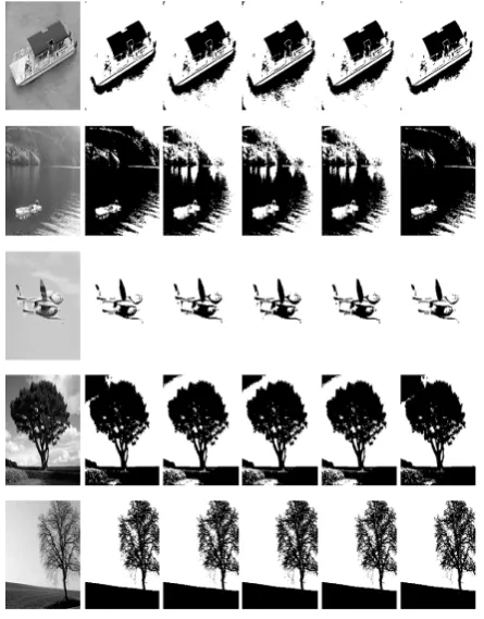
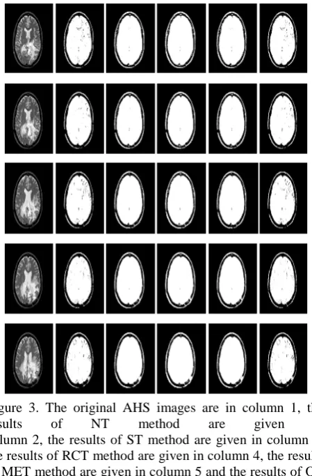
The comparisons of these five thresholding methods are done by using the final binary images produced by them. In Fig.1, the general gray images (GGI) are given in column 1, the results of NT method are given in column 2, the results of ST method are given in column 3, the results of RCT method are given in column 4, the results of MET method are given in column 5 and the results of OT method are given in column 6. In Fig.2, the normal MRI head scans (NHS) are given in column 1, the results of NT method are given in column 2, the results of ST method are given in column 3, the results of RCT method are given in column 4, the results of MET method are given in column 5 and the results of OT method are given in column 6. In Fig.3, the abnormal MRI head scans (AHS) are given in column 1, the results of NT method are given in column 2, the results of ST method are given in column 3, the results of RCT method are given in column 4, the results of MET method are given in column 5 and the results of OT method are given in column 6. The performance measure RNU is computed for GGI and values are shown in Table 1. RNU value of well segmented image is close to 0. MET provides well segmented images by having RNU value is 0.1229 and it has more close to 0 while comparing with other thresholding methods. The RNU values of NHS are shown in Table 2. In this case, RNU of RCT value is similar to the OT, but higher than OT RNU value. RNU value of OT is 0.3213 and its close to 0. This thresholding method given best results for NHS. The RNU values of AHS are shown in Table 3. RNU of OT is close to 0 while comparing with other thresholding methods for AHS.

Figure 1. The original GGI images are in column 1, the results of NT method are given in column 2, the results of ST method are given in column 3, the results of RCT method are given in column 4, the results of MET method are given in column 5 and the results of OT method are given in column 6.

Figure 3. The original AHS images are in column 1, the results of NT method are given in column 2, the results of ST method are given in column 3, the results of RCT method are given in column 4, the results of MET method are given in column 5 and the results of OT method are given in column 6.

Table 1: RNU values of GGI

General

Images NT ST RCT MET OT

GGI_1 0.1168 0.1286 0.0916 0.1747 0.0893

GGI_2 0.1068 0.1068 0.1057 0.0922 0.1057

GGI_3 0.004 0.0041 0.0047 0.0042 0.0048

GGI_4 0.4399 0.4435 0.4551 0.22 0.4551

GGI_5 0.1614 0.1537 0.2648 0.0332 0.2648

GGI_6 0.2931 0.2919 0.6622 0.1512 0.6488

GGI_7 0.8443 0.8405 0.7189 0.5834 0.7189

GGI_8 0.0042 0.0042 0.0042 0.0044 0.0042

GGI_9 0.4545 0.4439 0.6287 0.2219 0.6069

GGI_10 0.0759 0.0782 0.0729 0.0993 0.0729

GGI_11 0.1829 0.1658 0.4538 0.09 0.4538

GGI_12 0.1446 0.3071 0.3231 0.109 0.3082

GGI_13 0.0468 0.0554 0.0546 0.0118 0.0546

GGI_14 0.4112 0.4135 0.3345 0.2046 0.3345

GGI_15 0.0372 0.0468 0.0265 0.0222 0.0268

GGI_16 0.0253 0.0263 0.0295 0.0273 0.0295

GGI_17 0.3747 0.3758 0.4945 0.0889 0.2594

GGI_18 0.1047 0.1143 0.1201 0.0752 0.1184

Mean 0.2126 0.2222 0.2691 0.1229 0.2531

Table 2: RNU values of NHS

Normal MRI Head Scans

NT ST RCT MET OT

NHS_1 0.7467 0.6971 0.5511 0.7876 0.5455

NHS _2 0.6331 0.5709 0.4063 0.6797 0.3995

NHS _3 0.5974 0.5693 0.4184 0.6726 0.4053

NHS _4 0.5777 0.541 0.4168 0.6474 0.4076

NHS _5 0.4909 0.4566 0.32 0.5933 0.3125

NHS _6 0.4187 0.3787 0.3266 0.5201 0.3183

NHS _7 0.3494 0.3222 0.2896 0.4563 0.2738

NHS _8 0.2906 0.2809 0.2534 0.3912 0.2412

NHS _9 0.2514 0.2411 0.2169 0.3562 0.2086

NHS _10 0.2723 0.2646 0.2518 0.3669 0.2443

NHS _11 0.28 0.2717 0.2705 0.3751 0.2682

NHS _12 0.3041 0.2984 0.2946 0.3891 0.2891

NHS _13 0.3374 0.3325 0.328 0.4106 0.317

NHS _14 0.3005 0.2884 0.2824 0.372 0.2773

NHS _15 0.294 0.279 0.2863 0.3542 0.2582

NHS _16 0.3075 0.2921 0.2862 0.3646 0.2762

NHS _17 0.3753 0.3531 0.3466 0.4236 0.3391

NHS _18 0.4531 0.4343 0.4144 0.4847 0.4031

Mean 0.4044 0.3817 0.3311 0.4802 0.3213

Table 3: RNU values of AHS

Abnormal MRI Head Scans

NT ST RCT MET OT

AHS_1 0.8374 0.7942 0.73 0.9288 0.7256

AHS _2 0.8083 0.7722 0.6735 0.9121 0.6753

AHS _3 0.7073 0.6768 0.5907 0.8562 0.5853

AHS _4 0.6775 0.648 0.5517 0.8228 0.5517

AHS _5 0.6763 0.6159 0.5443 0.8195 0.5443

AHS _6 0.6129 0.5772 0.4899 0.7706 0.4899

AHS _7 0.5275 0.4841 0.413 0.7052 0.413

AHS _8 0.538 0.4919 0.4258 0.7084 0.4221

AHS _9 0.5001 0.4686 0.4158 0.6781 0.4083

AHS _10 0.4411 0.4094 0.3588 0.6137 0.355

AHS _11 0.4174 0.3826 0.3344 0.5876 0.3325

AHS _12 0.3974 0.3623 0.3147 0.562 0.3114

AHS _13 0.3572 0.3386 0.2902 0.5326 0.284

AHS _14 0.3658 0.34 0.312 0.5273 0.3075

AHS _15 0.3934 0.3704 0.3502 0.5696 0.3459

AHS _16 0.411 0.393 0.3749 0.5671 0.3712

AHS _17 0.429 0.3969 0.3925 0.6018 0.3932

AHS _18 0.4089 0.3891 0.4048 0.603 0.4035

We observed some different features by comparing these thresholding methods. Each thresholding methods have merits and demerits for their developed algorithm. Kittler and Illingworth’s thresholding given well segmented images for general gray images. This thresholding is not providing good results for both NHS and AHS. OT method is given well segmented images for both NHS and AHS.

5. CONCLUSION

This paper analyse the five thresholding methods to select robust thresholding technique for gray image binarization. Experiments were done on general images, normal and abnormal MRI head scans. The outputs generated by these methods were compared using RNU measure. Kittler and Illingworth’s thresholding technique provides better results for general gray images. Otsu’s thresholding finds to produce better quality of results when compared to other methods while considering both normal and abnormal MRI head scans.

REFERENCES

[1] Roy S, Dey A, et.al, “A New Efficient Binarization Metohd for MRI of Brain Image”, Signal and Image Processing: An Internation Journal, vol.3, no.6, 2012, pp.35-51.

[2] Kalaiselvi T. and Nagaraja P., “A rapid Automatic Brain Tumor Detection Method for MRI Images using Modified Minimum Error Thresholding Technique”, International Journal of Imaging Systems and Technology, vol.25, 2015, pp.77–85.

[3] Kalaiselvi T. and Nagaraja P., “Modified kittler and illingworth’s thresholding for MRI brain image segmentation”, Proceedings of International Conference MIKE-2013, Lecture Notes on Artificial Intelligence, Springer, Vol.8284, 2013, pp. 173–179, India.

[4] Al-amri S S, Kalyankar N V and Khamitkar S D, “Image Segmentation using threshold techniques”, Journal of Computing, vol.2, 2010, pp.83-86.

[5] Sauvola J and Pietikainen M, “Adaptive Document Image Binarization, Pattern Recognition”, 2000, vol.33, no.2, pp.225-236.

[6] Niblack J, “An Introduction to Digital Image Processing”, Prentice Hall, Eaglewood Cliffs, 1986, pp. 115-116.

[7] Bernsen J, “Dynamic Thresholding of Gray Level Images”, In: ICPR’86: Proceedings of the International Conference on Pattern Recognition, 1986, pp. 1251-1255.

[8] Kapur J N, Sahoo P K and Wong A K C, “A New Method for Gray-Level Picture Thresholding Using the Entropy of the Histogram”, Computer Vision, Graphics, And Image Processing 29, 1985, pp.273-285.

[9] Nikolaos N and Dimitris V, “A Binarization Slgorithm for Historical Manuscripts”, 12th wseas international conference on communications, Heraklion, Greece, July 23-25, 2008, pp.41-51.

[10] Shaikh S H, Maiti A K and Chaki N, “A New Image Binarization Method using Iterative Partitioning”, Springer- Machine Vision and Applications, 2012.

[11] Sezgin M. and Sankur B., “Survey Over Image thresholding Techniques and Quantitative Performance Evaluation”, Journal of Electronic Imaging, vol.13, no.1, 2004, pp.146-165.

[12] Sauvola J., Seppanen T., Haapakoski S., and Pietikainen M., “Adaptive Document Binarization”, 4th Int. Conf. On Document Analysis and Recognition, Ulm, Germany, pp.147-152 (1997).

[13] Ridler, T.W. and Calvard, S., “Picture Thresholding using and Iterative Selection Method”, IEEE Transactions of Systems, Man and Cybernetics, vol.8, no.8, 1978, pp.630-632.

[14] Kittler J and Illingworth J, “Minimum Error Thresholding, Pattern Recognition”, 19, 1979, pp 41-47.

[15] Otsu N, “A Threshold Selection from Gray level Histograms”, IEEE Transactions of Systems, Man and Cybernetics, vol.9, no.1, 1979, pp. 62-66.

[16] Kalaiselvi T. and Nagaraja P., “A Robust Thresholding Technique for Image Segmentation from Gray Images”, In Proceedings of the International Conference on Applied Mathematics and Theoretical Computer Science, vol.1, 2013. pp.183-188.

[17] Kalaiselvi T. and Nagaraja P. and Sriramakrishnan, P., “A simple image processing approach to abnormal slices detection from MRI tumor volumes, International Journal of Multimedia and Its Applications”, vol.8, 2016, pp.55–64. [18] Segmentation Evaluation Database, Department of

Computer Science and Applied Mathematics, Weizmann Institute of Science, Israel.