Interval B-Spline Curve Fitting

(1)

International Journal of Video&Image Processing and Network Security IJVIPNS-IJENS Vol:14 No:06 1

Interval B-Spline Curve Fitting

O. Ismail, Senior Member, IEEE

Abstract— Computing a curve to approximate data points is a problem encountered frequently in many applications in computer graphics, computer vision, CAD/CAM, and image processing. In this paper the concept of interval B-spline curve fitting is introduced. The four fixed Kharitonov's polynomials (four fixed B-spline curves) associated with the set of given interval data points and the interval B-spline curve are obtained. Then the problem is converted into determining a set of fixed control points that generates a B-spline curve for a set of given four fixed Kharitonov's polynomials (four fixed B-spline curves) associated with the interval data points. The problem of choosing the parameter value and the knot vector is also discussed, and how their choice affects the shape and parameterization of the curve. Where an improper data parameterization may considerably compromise the quality and efficiency of approximation. Finally the interval control polygon is obtained from the calculated fixed control polygons. A numerical example is included in order to demonstrate the effectiveness of the proposed method.

Index Term— Interval curve fitting, interval B-spline curve, computer graphics, image processing, CAGD.

I. INTRODUCTION

Curve fitting is important in computer graphics, computer-aided design, pattern recognition, and image processing [1-10]. The task of curve fitting is to construct a smooth curve that fits a set of given points in the space. In practice, a curve-fitting algorithm should meet two criterions: First, adjusting a control point of the curve affects only its vicinity, and second, it should be fast enough to be incorporated into an interactive program.

When the data exhibit a complicated shape, simple polynomials fall short, in this case, piecewise polynomials or polynomial splines are often chosen as parametrization for the underlying function [11], [12].

All existing CAD/CAM systems provide users with curve entities, which can be classified into Analytic and Synthetic entities. Analytic entities are points, lines, arcs, circles, fillets, chamfers and conics. Synthetic entities include cubic spline, B-spline and Bezier curves. Mathematically, synthetic curves represent problems of constructing smooth curves that passes through given data points. Therefore the typical form of these curves is a polynomial. Bezier and B-spline curves can approximate or interpolate the data points.

The B-spline stands as one of the most efficient curve representation, and possesses very attractive properties such as spatial uniqueness,

The author is with Department of Computer Engineering, Faculty of Electrical and Electronic Engineering, University of Aleppo, Aleppo,

(e-mail:[email protected]).

boundedness and continuity, local shape controllability, and structure preservation under affine transformation [13]. Because of these properties they can be used for represent curves.

B-splines are like Bezier curves because they both use a control polygon to define the curve, and are helpful due to their control points, local control of the resulting shape. The B in B-spline stands for ”basis”, and the basis is specified by the Cox-de Boor formula for computing the basis function. What uniquely sets them apart from Bezier curves is that a vector of scalars called a knot vector is figured in to the computation of the basis functions. When these knots are spaced evenly, the B-spline is said to be uniform, and nonuniform otherwise. The basis function considers the knot vector in every computation.

The B-spline curve overcomes the main disadvantages of the Bezier curve which are (1) the degree of the Bezier curve depends on the number of control points, (2) it offers only global control, and (3) individual segments are easy to connect with continuity, but is difficult to obtain. The B-spline curve features local control and any desired degree of continuity. To obtain continuity, the individual spline segments have to be polynomials of degree . The B-spline curve is an approximating curve and is therefore defined by control points. However, in addition to the control points, the user has to specify the values of certain quantities called “knots”. They are real numbers that offer additional control over the shape of the curve.

There are several types of B-splines. In the uniform (also called periodic) B-spline, the knot values are uniformly spaced and all the weight functions have the same shape and are shifted with respect to each other. In the nonuniform B-spline, the knots are specified by the user and the weight functions are generally different. There is also an open uniform B-spline, where the knots are not uniform but are specified in a simple way. The B-spline is an approximating curve based on control points, but there is also an interpolating version that passes through the points.

(2)

An interval B-spline curve is uniquely defined by its degree, interval control points and knot values. The modification of a curve plays a central role in CAD systems, hence numerous methods are presented to control the shape of a fixed B-spline curve by modifying one of its data mentioned above.

Parametric interval B-spline curves are interactive. It is possible to control the shape of the interval B-spline curve by moving the interval control points and by smoothly connecting individual interval segments. Imagine a situation where the interval points are moved and maneuvered for a while, but the interval curve “refuses” to get the right shape. This indicates that there are not enough interval points. When there are not enough control points, more control points need to be inserted to provide sufficient degree of freedom of a B-spline curve in order to achieve the desired approximation accuracy. When there are redundant control points, some control points need to be deleted in order to yield a compact B-spline fitting curve [15].

The B-spline curve fitting problem is to produce a B-spline curve to approximate a target curve within a prespecified tolerance. We assume that the target curve is defined in 2D plane by a sequence of ordered dense data points or a curve given implicitly or explicitly (i.e., by a parametric equation).

This paper is organized as follows. Section contains the basic results, whereas section shows numerical example, and the final section offers conclusions.

II. THEBASICRESULTS

Let ( ) be the position vector along the interval curve as a function of the parameter , an interval B-spline curve is given by:

( ) ∑,

( )

with knot vector * +, where the , - for ( ) are the interval position vectors of the ( ) interval control polygon vertices, and the are the normalized B-spline basis functions.

For the normalized B-spline basis function of order ( ), the basis functions ( ) are defined by the Cox-de Boor recursion formulas [16]. Specifically:

( ) { } ( )

( ) ( )

( )

The values of are elements of a knot vector satisfying the relation . The parameter varies

from to along the interval curve ( ). The convention ( ⁄ ) is adopted. Formally, a B-spline curve is defined as a polynomial spline function of order ( ), because it satisfies the following two conditions: ( ) ( ) is an interval polynomial of degree ( ) on each interval . ( ) ( ) and its derivatives of order ( ) are all continuous over the entire interval curve.

Vector-valued interval ( ) in the most general terms is defined as any compact set of points ( ) dimensions as tensor products of scalar intervals:

, - , - *( ) , - , -+ ( )

such vector-valued intervals are clearly just rectangular regions in plane [17].

For each , the value ( ) of the interval

curve ( ) is an interval vector that has the following significance: For any fixed curve ( ) whose control points satisfy , - for ( ) we have

( ) ( ) . Likewise, the entire interval curve ( ) defines a region in the plane that contains all curves whose control points satisfy , - for ( ).

We are given a set of interval data points , -, , -, , [ ]. The problem is to determine a set of interval control points that generates an interval B-spline curve for a set of given interval data points. If an interval data point belong to the interval B-spline curve, then it must satisfy equation ( ). Writing equation ( ) for each of interval data points yields:

, -( ) ( ), - ( ), - ( ) ( ), -, -( ) ( ), - ( ), - ( ) ( ),

-, -( ) ( ), - ( ), - ( ) ( ),

( )

The four fixed Kharitonov's polynomials (four fixed B-spline curves) , - associated with both sides of equation ( ) are:

( ) ( ) ( ) ( ) ( )

( ) ( ) ( ) ( ) ( ) ( ) ( ) ( ) ( )

( ) ( ) ( ) ( ) ( )

( ) ( ) ( ) ( ) ( ) ( ) ( ) ( ) ( )

( ) ( ) ( ) ( ) ( )

( ) ( ) ( ) ( ) ( ) ( ) ( ) ( ) ( )

( ) ( ) ( ) ( ) ( )

(3)

( ) ( ) ( ) ( ) ( )

( ) ( ) ( ) ( ) ( ) ( ) ( ) ( ) ( )

( ) ( ) ( ) ( ) ( )

( ) ( ) ( ) ( ) ( ) ( ) ( ) ( ) ( )

( ) ( ) ( ) ( ) ( )

( ) ( ) ( ) ( ) ( ) ( ) ( ) ( ) ( )

( ) ( ) ( ) ( ) ( )

( ) ( ) ( ) ( ) ( ) ( ) ( ) ( ) ( )

( ) ( ) ( ) ( ) ( )

( ) ( ) ( ) ( ) ( ) ( ) ( ) ( ) ( )

( ) ( ) ( ) ( ) ( )

( ) ( ) ( ) ( ) ( ) ( ) ( ) ( ) ( )

( ) ( ) ( ) ( ) ( )

( ) ( ) ( ) ( ) ( ) ( ) ( ) ( ) ( )

( ) ( ) ( ) ( ) ( )

( ) ( ) ( ) ( ) ( ) ( ) ( ) ( ) ( )

( )

Now, the problem can be formulated as follows: determine a set of fixed control points that generates a B-spline curve for a set of given four fixed Kharitonov's polynomials (four fixed B-spline curves) associated with the interval data points. If a fixed data point belong to the B-spline curve, then it must satisfy equation ( ).

Equation ( ) can be rewritten as follows:

( ) ∑ _{( )}

( )

( ) ( ) ( )

for ( ).

This system of equations can be rewritten in matrix form as:

( )

where,

[

( ) ( ) ( ) ( )

( ) ( ) ( ) ( )]

, - , ( ) ( ) (

)-, - [ ( ) ( ) ( ) ( )] ( ) ( )

Formally, an open uniform knot vector is given by:

{

} ( )

The problem of choosing the parameter value and the knot vector remains, and their choice affects the shape and parameterization of the curve. Assigning parameter values to data points, a procedure to be referred to as data parameterization. Different ways of data parameterization lead to different approximation results. Fundamentally, the notion of the optimal data parameterization is theoretically elusive and computationally difficult to achieve. An improper data parameterization may considerably compromise the quality and efficiency of approximation. The following three methods for data parameterization have been proposed [19], [20], [21] for choosing the

- Uniformly spaced method:

For parameters to be equally spaced in , -, we have:

( )

This assignment scheme, though simple, does not work well when the control points are placed unevenly. In such cases, curves with unsatisfactory shapes might result.

- Chord length method:

To ensure that the curve shape closely follows the shape of the corresponding polyline, this method of parameterization may be employed. Herein, parameters are placed proportional to the chord lengths of control polyline, that is, if the first parameter corresponding to is , then the subsequent parameters corresponding to may be written as:

∑

( )

We may normalize the parameterization in equation ( ) by setting to and dividing by the total chord length of the polyline:

∑

( )

(4)

( ) [∑

∑

⁄ ]

( )

The chord length method is widely used and it usually performs well. Sometimes, a longer chord may cause its curve segment to have a bulge bigger than necessary, which is a common problem with the chord length method. It also gives a „good‟ parameterization to the curve, in the sense that it approximates a uniform parameterization.

- Centripetal method:

This is derived from a concept analogous to the centripetal acceleration when a point is traversing along a curve. The notion is that the centripetal acceleration should not be too large at sharp turns (smaller radii of curvature). For the parameters to lie in the domain , -, the centripetal method gives the parameter values as:

( ) [∑

∑

⁄ ]

( )

with as . Note that equations ( ), ( ) and ( ) can be generalized to:

( ) [∑

∑

⁄ ]

( )

for some chosen exponent . For , uniformly spaced parameterization is obtained while for and ⁄ , respectively, chord length and centripetal parameterizations are achieved.

Knot can be equally spaced, that is,

{

} ( )

However, this method is not recommended; if used in conjunction with equations ( ) and ( ) it can result in a singular system of equations described by equation( ). We recommend the following technique of averaging:

{

∑

}

( )

With this method the knots reflect the distribution of the .

The maximum parameter value, , is usually taken as

the maximum value of the knot vector.

If ( ) , then the matrix is square and the fixed control polygons are obtained directly by matrix inversion, i.e.,

( )

In this case, the resulting fixed B-spline curves pass through each data point; i.e., a fixed curve fit is obtained. Although the continuity of the resulting fixed curves is everywhere , it may not be „smooth‟. The fitted fixed curves may develop unwanted wiggles or undulations.

Finally, the interval control polygon *, -+ is obtained from the calculated fixed control polygons as follows:

, - [ ( _{( )}) ( _{( )}) ] ( ) ( ) ( )

A smoother fixed curves can be obtained by specifying fewer fixed control polygon points than fixed data points, i.e., ( ). Here, is no longer square; the problem is over specified and can only be solved in a mean sense. Recalling that a matrix times its transpose is always square, the fixed control polygons for a fixed B-spline curves that smooths the data is given by:

, -

( )

and the interval control polygon *, -+ is obtained from equation ( ).

Both of these techniques assume that the matrix is known. Provided that the order of the B-spline basis , the number of control polygon vertices , and the parameter values along the curve are known, then the basis functions ( ) and hence the matrix can be obtained. Within the restrictions( ), the order and number of polygon vertices are arbitrary.

III. NUMERICALEXAMPLE

(5)

International Journal of Video&Image Processing and Network Security IJVIPNS-IJENS Vol:14 No:06 5 , - (, - , -)

, - (, - , -) , - (, - , -) , - (, - , -) , - (, - , -)

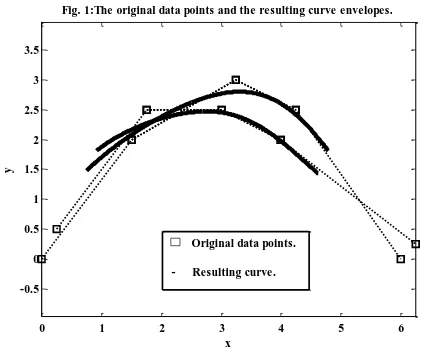
Determine the third-order ( ) interval control polygon having five and four interval polygon vertices that generate an interval B-spline curve „through‟ the given interval data points. Use the chord length approximation for the parameter values along the interval B-spline curve corresponding to the given interval data points.

First, determine the chord lengths:

| |

⁄

∑( )

For five polygon vertices, the maximum value of the knot vector for a third-order B-spline curve is , where is one less than the number of polygon vertices. The knot vector with multiplicity at the ends is:

,

-As explained in section II, the five fixed control points,

for ( ) and ( )of the four fixed

Kharitonov's polynomials (four fixed B-spline curves) are obtained as shown in table:

( ) ( ) ( ) ( ) ( ) ( ) ( ) ( ) ( ) ( ) ( ) ( ) ( ) ( ) ( ) ( ) ( ) ( ) ( ) ( )

and the interval control points *, -+are obtained from the above fixed control points as follows:

, - (, - , -) , - (, - , -) , - (, - , -) , - (, - , -) , - (, - , -)

Simulation results in Figure 1 shows the envelopes of original data points, the calculated control polygon and the resulting curve.

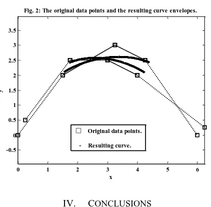
For four polygon vertices, the knot vector with multiplicity at the ends is:

,

-The four fixed control points, for ( ) and ( ) of the four fixed Kharitonov's polynomials (four fixed B-spline curves) are obtained as shown in table:

( ) ( ) ( ) ( ) ( ) ( ) ( ) ( ) ( ) ( ) ( ) ( ) ( ) ( ) ( ) ( )

and the interval control points *, -+ are obtained from

the above fixed control points as follows:

0 1 2 3 4 5 6

-0.5 0 0.5 1 1.5 2 2.5 3 3.5

x

y

Fig. 1:The original data points and the resulting curve envelopes.

Original data points.

(6)

International Journal of Video&Image Processing and Network Security IJVIPNS-IJENS Vol:14 No:06 6 , - (, - , -)

, - (, - , -) , - (, - , -) , - (, - , -)

Simulation results in Figure 2 shows the envelopes of original data points, the calculated control polygon and the resulting curve.

IV. CONCLUSIONS

Fitting a curve to a set of data points is a fundamental problem in graphics and many other application areas. Approximating measured data by a smooth curve is a frequent problem in motion analysis, computer aided design, image processing and many other fields. When the data exhibit a complicated shape, simple polynomials fall short. In this case, piecewise polynomials or polynomial splines are often chosen as parameterization for the underlying function. The concept of interval B-spline curve fitting is introduced in this paper. The four fixed Kharitonov's polynomials (four fixed B-spline curves) associated with the set of given interval data points and the interval B-spline curve are obtained. Then the problem is converted into determining a set of fixed control points that generates a B-spline curve for a set of given four fixed Kharitonov's polynomials (four fixed B-spline curves) associated with the interval data points. The problem of choosing the parameter value and the knot vector is also discussed, and how their choice affects the shape and parameterization of the curve. Where an improper data parameterization may considerably compromise the quality and efficiency of approximation. Finally the interval control polygon is obtained from the fixed control polygons.

REFERENCES

[1] T. Pavlidis, “Curve fitting with conic splines” ACM Transactions on Graphics, Vol. 2, pp. 1–31, 1983.

[2] M. Plass and M. Stone, “Curve-fitting with piecewise parametric cubics”, Computer Graphics, Vol. 17, No. 3, pp. 229–239, 1983. [3] V. Pratt, “Techniques for conic splines”, „Proceedings of

SIGGRAPH‟85, pp. 151–160, 1985.

[4] DF. Rogers and NG. Fog, “Constrained B-spline curve and surface fitting”, Comput Aided Geom. Des., Vol. 21, pp. 641–648, 1989A.

[5] P. Dierckx, Curve and surface fitting with splines. Oxford: Clarendon

Press; 1993.

[6] R. D. Forsey and R. H. Bartels, “Surface fitting with hierarchical splines”, ACM Transactions on Graphics, Vol. 14, pp. 134–161, 1995.

[7] W. Ma, and JP. Kruth, “Parametrization of randomly measured points for the least squares fitting of B-spline curves and surfaces”, Comput. Aided Des., Vol. 27, pp. 663–675, 1995.

[8] G. Farin, Curves and surfaces for computer aided geometric design: A practical guide, Academic Press, New York, 4th edition, 1997.

[9] A. A. Goshtasby, “Grouping and parameterizing irregularly spaced points for curve fitting”, ACM Transactions on Graphics, Vol. 19, pp. 185–203, 2000.

[10] V. Weiss, L. Andor, G. Renner, and T. Varady, “Advanced surface fitting techniques”, Computer Aided Geometric Design, Vol. 19, pp. 19–42, 2002.

[11] D. J. Walton and R. Xu, “Turning point preserving planar interpolation”, ACM Transactions on Graphics, Vol. 10, pp. 297 – 311, 1991.

[12] P. Dierckx. Curve and surface fitting with splines. Oxford University Press, Inc., New York, NY, USA, 1993. ISBN 0-19-853441-8.

[13] C. de Boor, “On Calculation with B-splines”, J. Approx. Theory Vol. 6, pp. 50-62, 1972.

[14] G. Shen and N. M. Patrikalakis, “Numerical and geometrical properties of interval B-spline”, International journal of shape modeling, Vol. 4, No. (1/2), pp. 35-62, 1998.

[15] H. P. Yang, W. Wang, and J. G. Sun, “Control point adjustment for B-spline curve approximation”, Computer-Aided Design, Vol. 36, pp. 639–652, 2004.

[16] Carl de Boor. A practical guide to splines. Springer-Verlag, New York, revised edition, 2001.

[17] T. W. Sederberg and R. T. Farouki, “Approximation by interval Bezier curves”, IEEE Comput. Graph. Appl., No, 2, Vol. 15, pp. 87-95, 1992.

[18] V. L. Kharitonov, "Asymptotic stability of an equilibrium position of a family of system of linear differential equations", Differential 'nye Urauneniya, vol. 14, pp. 2086-2088, 1978.

[19] H. Park, “Choosing nodes and knots in closed B-spline curve interpolation to point data”, Comput. Aided Des., Vol. 33, No. 13, pp. 967–74, 2001.

[20] TI. Vassilev, “Fair interpolation and approximation of B-splines by energy minimization and points insertion”, Comput. Aided Des., Vol. 28, No. 9, pp. 753– 60, 1996.

[21] X. Wang, F. Cheng, and BA. Barsky, “Energy and B-spline interapproximation”, Comput. Aided Des., Vol. 29, No. 7, pp. 485– 96, 1997.

O. Ismail (M‟97–SM‟04) received the B. E. degree in electrical and

electronic engineering from the University of Aleppo, Syria in 1986. From 1987 to 1991, he was with the Faculty of Electrical and Electronic Engineering of that university. He has an M. Tech. (Master of Technology) and a Ph.D. both in modeling and simulation from the Indian Institute of Technology, Bombay, in 1993 and 1997, respectively. Dr. Ismail is a Senior Member of IEEE. Life Time Membership of International Journals of Engineering & Sciences (IJENS) andResearchers Promotion Group (RPG). His main fields of research include computer graphics, computer aided analysis and design (CAAD), computer simulation and modeling, digital image processing, pattern recognition, robust control, modeling and identification of systems with structured and unstructured uncertainties. He has published more than 66 refereed journals and conferences papers on these subjects. In 1997 he joined the Department of Computer Engineering at the Faculty of Electrical and Electronic Engineering in University of Aleppo, Syria.

0 1 2 3 4 5 6

-0.5 0 0.5 1 1.5 2 2.5 3 3.5

x

y

Fig. 2: The original data points and the resulting curve envelopes.

Original data points.

(7)

In 2004 he joined Department of Computer Science, Faculty of Computer Science and Engineering, Taibah University, K.S.A. as an associate professor for six years.

He has been chosen for inclusion in the special 25th Silver Anniversary Editions of Who‟s Who in the World. Published in 2007 and 2010.