MULTIPLE EQUILIBRIA
IN
THEORY AND PRACTICE
Ahmed Waqar Anwar
University College London
Department of Economics
Thesis submitted for the degree of
Doctor of Philosophy
University of London
ProQuest Number: U643541
All rights reserved
INFORMATION TO ALL USERS
The quality of this reproduction is dependent upon the quality of the copy submitted. In the unlikely event that the author did not send a complete manuscript and there are missing pages, these will be noted. Also, if material had to be removed,
a note will indicate the deletion.
uest.
ProQuest U643541
Published by ProQuest LLC(2016). Copyright of the Dissertation is held by the Author. All rights reserved.
This work is protected against unauthorized copying under Title 17, United States Code. Microform Edition © ProQuest LLC.
ProQuest LLC
789 East Eisenhower Parkway P.O. Box 1346
Acknowledgements
ABSTRACT
The first part o f the thesis studies equilibrium selection. We use a stochastic evolutionary model characterised by small probability shocks or mutations which perturb the system away from its deterministic evolution, allowing it to move between equilibria over a long period o f time. Much o f the literature has concentrated on the result that, in the hmit as the mutation rate approaches zero, the stationary distribution becomes concentrated on the risk-dominant equilibrium because it is easier to flow into. However, it has been shown that in models o f local interaction, allowing player movement eases the flow into the efficient equihbrium. We look at the consequences o f such player movement when there are capacity constraints which limit the number o f agents who can reside at each location. The limit distribution may then become concentrated on a mixed state in which different locations coordinate on different equilibria.
Contents
List o f figures
List o f tables
1
Introduction
91.1
The Equilibrium Selection
Problem 111.1.1 Equilibrium Refinements 11
1.1.2 The Evolutionary Approach 15
1.2
Equilibria in Multi-Unit Auctions
23
1.3
Summary o f Results
32
2
Equilibrium Selection in Games
352.1
Stochastic Techniques
40
2.1.1 Friedlin and Wentzell 40
2.1.2 Kandori, Mailath and Rob 42
2.1.3 Young 46
2.2
When D oes Immigration Facilitate Efficiency
47
2.2.1 Two Islands 47
2.2.3 Inertia in Strategy Revision 62
2.2.4 No Capacity Constraints 65
2.3
Conclusions
67
2.4
Appendix
68
Multi-Unit, Common-Value Auctions
73
3.1
Multiple Equilibria in Uniform-price,
Multi-Unit Auctions
76
3.2
Discrete Units
79
3.3
Capacity Constraints and Uncertain
Demand
83
3.3.1 Discriminatory Auction 84
3.3.2 Uniform-price Auction 94
3.3.3 Ranking 100
3.4
Conclusions
103
3.5
Appendix
105
4
Modelling the Electricity Pool
107
4.1
Price Determination Process in
4.2
Electricity Pool Literature
114
4.2.1 Green and Newbery 114
4.2.2 von der Fehr and Harbord 119
4.2.3 Wolak and Patrick 123
4.3
The Case for a Discriminatory Auction
in the England and Wales Pool
126
4.3.1 A model o f the England and Wales
Pool 127
4.3.2 Alternative Pricing Rules 141
4.3.3 Ranking the Pricing Rules in the
England and Wales Pool 144
4.3.4 Repeated Game Analysis 146
4.4
Conclusions
148
4.5
Appendix
150
List o f figures.
Figure 1.1 12
Figure 1.2 14
Figure 2.1 42
Figure 2.2 45
Figure 2.3 47
Figure 2.4 53
Figure 2.5 53
Figure 2.6 56
Figure 2.7 60
Figure 2.8 60
Figure 2.9 61
Figure 2.10 64
Figure 2.11 70
Figure 3.1 76
Figure 3.2 78
Figure 3.4 80
Figure 4.1 116
Figure 4.2 117
Figure 4.3 130
Figure 4.4 133
Figure 4.5 134
Figure 4.6 135
Figure 4.7 150
Figure 4.8 152
Figure 4.9 152
List o f tables.
Table 2.1 54
Table 4.1 151
Chapter 1
Introduction
The first part o f the thesis looks at the question o f equilibrium selection. The limitations o f the early approach o f equilibrium refinements is illustrated by the failure o f this literature to predict equilibrium play correctly in numerous laboratory experiments. M ost o f the literature also ignores the question of selecting between strict Nash equilibria. Evolutionary game theory addresses the question o f equilibrium selection by modelling the way agents adjust their strategies out o f equilibrium. The evolutionary approach has been successful both in explaining some o f the experimental evidence and addressing the question of selecting between strict Nash equilibria. These ideas are discussed in more detail in section 1.1. In chapter 2, we address the question o f selecting between strict Nash equilibria. We present a stochastic evolutionary model with player movement and capacity constraints hmiting the number o f agents who can reside at each location.
1.1 The Equilibrium Selection Problem.
A Nash equilibrium is a set o f strategies such that each player is optimising given the strategies o f the other players. Nash (1950) showed that every finite game has at least one Nash equilibrium. A question that has been the focus of much research since is which equilibrium will be played when a game has multiple equilibria. The early approach was to refine the set o f equilibria by eliminating equilibria that are not plausible when the game is played by rational agents. This approach is briefly discussed in the next section. However, experimental evidence has shown that the predictions o f the equilibrium refinement literature are not always correct. Game theorists have turned instead to the evolutionary approach. By modelling how agents adjust their strategies out o f equilibrium we can analyse how a population settles on one o f the equilibria. This approach is discussed in section 1.1.2.
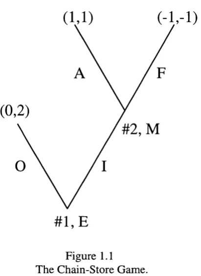
1.1.1 Equilibrium Refinements.
would be better off acquiescing.
(-
1
,-
1
)
(1,1)
(
0
,
2
)
# 2 , M
# 1 , E
Figure 1.1
The Chain-Store Game.
every information set. Selten defines a perfect equilibrium as one that arises when the mistake probability goes to zero. Myerson (1978) shows that adding strictly dominated strategies may change the set o f perfect equilibria and he introduces a further refinement. He postulates that rational players are more likely to make mistakes that are less costly. One o f many other refinements to the perfectness concept is strict perfectness (Okada 1981). A strictly perfect equilibrium is stable against arbitrary slight perturbations.
Kreps and W ilson (1982) take an alternative approach to refining subgame perfection. They assume that agents will maximise utility in the face o f uncertainty using subjective probabilities. Hence, when an information set that is not on an equilibrium path is reached, the agent will make a best reply according to his beliefs about the state o f the game. If there exists a set o f beliefs such that each player optimises by continuing to play according to the equilibrium, the equilibrium is sequential. For a comprehensive guide to the equilibrium refinement literature the reader is referred to van Damme (1991). Although the refinement literature has had some success in dealing with the question o f equilibrium selection it has tw o major problems: some o f the predictions o f the refinement literature have been refuted by experimental evidence; equilibrium refinements have nothing to say about the choice between strict equilibria.
game-theoretic predictions have performed much better when these conditions are satisfied (Ledyard 1995). However, there are some exceptions, the most notable o f which is the Ultimatum Game. Binmore, Gale and Samuelson (1995) argue that it was wrong for game theorists to assume that players would always play according to a subgame-perfect equilibrium, which is based on eliminating weakly dominated strategies. They use an alternative evolutionary approach based on interactive learning to explain the experimental outcomes. This is discussed in the next section.
The second difficulty with the equilibrium refinement approach is that it has nothing to say about the choice between strict equilibria. Consider the Coordination Game o f figure 1.2.
Si S2
S]
S2
5,5 0,3
3,0 4,4
Figure 1.2
The game has two strict pure-strategy equilibria, {si, s% j and {s2, S2},
equally likely to play either strategy, the outcome w ill be {S2, S2}, which
therefore also has a focal status that may outweigh that o f the payoff-dominant equilibrium. Evolutionary game theory has given the argument another perspective. By modelling the process by which agents adjust their strategies out o f equilibrium we can analyse how it is that one equilibrium is selected rather than another. In chapter 2, w e use an evolutionary model to address the question o f equilibrium selection in 2x2 Coordination Games.
1.1.2 The Evolutionary Approach
Evolutionary game theory was developed by biologists to model situations in which the fitness (or reproductive success) o f a gene depends on the current mix o f genes in the population. One can think of the evolutionary game as being played between genes which are programmed to give their host certain characteristics. Together with the current mix o f genes in the population, the fitness o f a gene is determined by these characteristics as the population o f hosts are competing for scarce resources. Genes that engender successful behaviour will therefore gain in frequency relative to those that result in lower reproductive success. A dynamic system known as the replicator dynamics (Taylor and Jonker 1978, Zeeman 1981) based on this type o f selection is derived below.
population is stable against invasion by a small number o f mutants.
To look at these ideas more formally w e need to introduce some notation. Consider a population o f agents who are randomly paired to play a symmetric two-player game, G. Let S=(S], s%,...s„) be the set o f pure strategies o f G. Denote the set o f mixed strategies by AS. The payoff to an agent using strategy x
against one using strategy y is given by P[x, y] where x,y e AS. Then Smith and Price define an ESS as a strategy x that satisfies the following two conditions
P[x,x] > P [ y ,x ] V y,
P[x, x] = P[y, x] => P[x, y] > P[y, y].
To get a more intuitive understanding o f an ESS consider the following alternative definition used by Taylor and Jonker (1978). A state x is an ESS if for every y # x and for a sufficiently small £>0
P [x,£y-l-(l-£)% ] > P [ y , e y - l - ( l - £ ) x ] .
small. Hence the experimenters will soon switch back to the convention. The ESS concept says nothing about how an equilibrium is reached. It simply gives a stability property that an equilibrium ‘should’ have.
The most commonly used dynamic system in the biological literature is the replicator dynamics o f Taylor and Jonker (1978). We now think o f players as being programmed with pure strategies. This differs from the ESS analysis which allows for mixed strategies. Let the number o f players programmed to use strategy Si at time t be p,(t) and X |( t ) be the corresponding proportion o f the population using the strategy. Hence the expected payoff to a player using strategy s, when randomly matched with someone in the population is
7=1
This is formally equivalent to playing against an opponent using the mixed strategy x(t)=(xi(t), X z ( t ) , X n (t)) with a payoff o f P[Si,x]. Similarly the average payoff in the population is P [x ,x ]. These proportions change over time as some o f the hosts die and new hosts programmed to use the strategy o f their single parent are bom. If reproduction takes place continuously over time then P[Sj, x(t)] represents the incremental effect on the birth rate from playing the game. If there is a background birth rate p that is independent o f the game and the death rate is
a , then the population dynamics is given by
P, (0 = [P
,XO] - ot]p, (0 .
derivative o f both sides o f the identity p(t)Xi(t)=pi(t) where p(t) is the size o f the
population at time t. This gives p{ t ) x i { t ) = p^ ( /) - p { t ) x^. Substituting for p^{t)
and p{t ) gives
( 0 = [P[Si, x{t)] - P[x{t),x(t)]x- (t) .
This derivation o f the standard continuous time replicator equation is given in Weibull (1995). The growth rate o f a strategy at any time is simply the difference between the payoff from using the strategy and the average payoff in the population.
population will settle on an equilibrium o f the game which is represented by a rest point o f the dynamics. Crucially, the equilibria that are selected in this way do not always correspond to those selected in the equilibrium-refinement literature. In particular weakly dominated equilibria are not necessarily eliminated.
The key lesson from this is that we cannot eliminate weakly dominated equilibria if the process by which an equilibrium is reached is evolutive in nature. The question o f equilibrium selection should then be addressed by modelling the dynamic process by which an equilibrium is reached. The replicator dynamics is used quite generally in a biological context but there is no reason to assume that a model o f strategy adjustment through interactive learning will lead to these dynamics. In fact, the dynamics will vary according to the assumptions made about the strategy adjustment process.
However, a surprising amount can be said about equilibrium selection with minimal assumptions on the dynamic process. If the dynamics are such that strategies that currently yield a higher than average payoff are used by a greater proportion o f the population in future periods, then the equilibrium the system converges to will simply depend on the point where the process began. In a 2x2 Coordination Game such as the one given in figure 1.2, if the process starts at a point where a significant number o f agents are playing strategy Si then the optimum response is to play S|. Agents who are using the other strategy will adjust their strategy when they learn that it is better to switch. The process will then converge on the equilibrium where everyone plays Si.
process is likely to follow the ‘learning’ dynamics and converge to one o f the equilibria o f the game. However, there will eventually be enough simultaneous mutations to move the system into the vicinity o f another equilibrium. The system is then likely to converge to this equilibrium and will remain there until it is once again moved by a large number o f simultaneous mutations. Over a long period of time one will find that the relative time spent in or close to some equilibria will be greater than others. Kandori et al (1993) and Young (1993) consider the limiting distribution, as the mutation rate is allowed to go to zero. They show the stationary distribution then becom es concentrated on a subset o f the equilibria and very often on a unique equilibrium. An equilibrium selected in this way is referred to as a long-run equilibrium. This is a very strong result when one considers the minimal assumptions made on the strategy adjustment process'.
The theoretical literature has concentrated attention on the 2x2 Coordination Game o f the type given in figure 1.2, where one equilibrium is risk-dominant and the other one is payoff-risk-dominant. D oes an evolutionary analysis pick Schelling’s payoff-dominant equilibrium or Harsanyi and Selten’s risk-dominant equilibrium? We focus on this question in chapter 2. In the models presented by Kandori et al and Young the unique long-run equilibrium o f the game is the risk-dominant equilibrium.
We explain the techniques used to characterise the limit o f the stationary distribution in section 2.1. W e present a model o f local interaction where agents are only paired with players from the same location in section 2.2. We consider
1.2 Equilibria in Multi-Unit Auctions.
In theory one can design the optimal mechanism for the sale o f multiple objects. By the Revelation Principle the designer can restrict attention to direct, incentive-compatible mechanisms. The problem o f multiple equilibria would not arise as the mechanism would be designed to elicit truthful revelation. In practice, relatively little is known about optimal mechanisms for the sale of multiple objects. A first step to obtaining a greater understanding is to compare mechanisms that are currently used. Even this has proved difficult however. In the sale o f Treasury bonds, for example, the US Treasury have switched between using a discriminatory auction and a uniform-price auction. In both cases the participants submit demand schedules reflecting the maximum price they are willing to pay for various quantities. These bids are used to construct the aggregate demand schedule and if the number o f bonds for sale is n then the n highest bids win. Under a discriminatory auction the bid price is paid for units won. With a uniform pricing rule, all winning bids pay the bid price o f the lowest winning bid. The question o f which one results in the higher revenue is still open.
It is well understood that the first-price auction and the Dutch auction are strategically equivalent as the bidders in a Dutch auction must simply decide the price at which they will stop the auction. In a model o f independent private values^, the second-price auction and the English auction are also equivalent. In the second-price auction it is a dominant strategy to submit a bid equal to your valuation, while in an English auction it is a dominant strategy to bid until the auction price reaches your valuation. Both auctions therefore result in an outcome that is efficient, as the object is sold to the bidder that values it most highly. The Dutch and first-price auctions also result in an efficient outcome as in equilibrium, all bidders shade their bids symmetrically. Moreover, in such equilibria the bidder who values the object most highly will optimise by bidding at the expected value o f the second highest bid. This gives the famous revenue equivalence result: the expected revenue to the seller is the same under all four auctions (Vickrey (1961), Myerson (1981)). In fact, with an optimally determined reserve price, the four auctions are also optimal mechanisms (Myerson (1981)). This result is one o f the major achievements o f mechanism design theory as it shows that there is no elaborate mechanism that will result in a higher expected revenue than the four simple auctions.
The prevalence o f the English auction in practice can be explained by relaxing the assumptions on which the Revenue Equivalence Theorem is based. For example, when bidders’ valuations are affiliated, the English auction yields a higher expected revenue than the other three auction formats (Milgrom and Weber 1982). The reason is that the English auction process conveys information
to the bidders on the valuations o f other bidders. Under the other three auction formats, no such information is conveyed and bidders therefore reduce their bids to account for the fact that they have the highest valuation if they win^. The first-price auction is also used widely in practice, and this can be explained by the fact that it performs better than the English auction if the bidders are risk-averse (Holt 1980). This is because under a first-price auction, bidders will increase their bids towards their valuation if they are risk-averse, to increase the probability that they win.
However, the English auction is not the optimal mechanism with affiliated values and the first-price auction is not the optimal mechanism when bidders are risk-averse. More elaborate mechanisms can be designed that increase the expected revenue to the seller. For example, when bidders are risk-averse the optimal auction involves subsidising high losing bidders and penalising low bidders (Maskin and Riley 1984). Such mechanisms are rarely observed in practice. One reason for this is that the optimal mechanism is difficult to characterise when a single assumption is relaxed. Hence most o f the literature concentrates on optimal mechanisms when just one or two assumptions are relaxed. The problem o f designing optimal mechanisms for complex economic environments is considered to be intractable. A second reason that elaborate mechanisms are rarely used in practice is that they are complicated relative to the simple auctions. Real economic agents are at best boundedly rational, unlike the idealised agents o f orthodox implementation theory. The rules o f the mechanism therefore need to be sufficiently simple for all to understand.
A great deal o f work has been done in extending the single-unit results to the case o f multiple units. The Revenue Equivalence Theorem extends to the case where there are multiple units and each bidder demands one unit (Harris and Raviv 1981, Maskin and Riley 1989). Maskin and Riley also investigate optimal auctions in the case that bidders demand multiple units and show that neither the discriminatory auction nor the uniform-price auction is optimal. However, as I pointed out earlier, elaborate mechanisms are not used in practice. The optimal auction can be complicated under simple assumptions even in the single-unit case. It is correspondingly more complicated in the multi-unit case. The problem of designing the optimal auction for the sale o f Treasury bonds is therefore very difficult and this is generally true o f complex economic environments.
The public debate on the mechanism used for the sale o f Treasury bonds has therefore concentrated on the choice between the discriminatory auction and the uniform-price auction. Even this question, however, remains unresolved. The conceptual difficulty o f multi-unit auctions is highlighted by a false analogy that is made between the second-price, sealed-bid auction for a single unit and a uniform-price auction for multiple units. For example McAfee and McMillan (1987) state: “Both the discriminatory auction and the uniform-price auction have been used to sell Treasury Bills. Because this is a common-value setting, theory predicts the uniform-price auction, which is similar to the second-price auction, yields more revenue than the discriminatory auction, which corresponds to the first-price auction”. The theory they are referring to is the affiliated valuations model o f Milgrom and Weber (1982).
by suggesting that under a uniform-price auction it is a dominant strategy to bid one’s true demand curve. In the Wall Street Journal (August 28, 1991) Friedman states: “A [uniform-price] auction proceeds precisely as a discriminatory auction with one cmcial exception: All successful bidders pay the same price, the cut-off price. An apparently minor change, yet it has the major consequence that no one is deterred from bidding by fear o f being stuck with an excessively high price. You do not have to be a specialist. You need only to know the maximum price you are willing to pay for different quantities.” Merton Miller in an interview with the N ew York Times explains why the bidders have an incentive to shade their bids under a discriminatory auction. He then says o f a uniform-price auction: “You just bid what you think it’s worth.” This argument was part o f the reason the US Treasury experimented with the uniform-price auction in the early 9 0 ’s. A report by the Treasury Department, the Securities and Exchange Commission and the Federal Reserve Board"^ concluded that: “Moving to a uniform-price award method permits bidding at the auction to reflect the true nature o f investor preferences..., In the case envisioned by Friedman, uniform-price awards would make the auction demand curve identical to the secondary market demand curve.” Recently Back and Zender (1993), Wang and Zender (1995), Ausubel and Crampton (1995) and Binmore and Swierzbinski (1997), have all illustrated that the bidders do have an incentive to shade their bids under a uniform pricing rule. The reason is there is a chance that one o f the bids o f a bidder will be the marginal bid that determines the uniform price. Bidders can reduce the price they pay for all the units they win in this event by shading bids. In fact, this was first noted by
Vickrey (1961), who also gives the correct multi-unit extension o f the second-price auction^. Back and Zender and Wang and Zender use the share auction framework o f Wilson (1979), where the good is perfectly divisible and has a common value. They find that any price between the reservation price and the lower bound o f the common-value distribution can be supported as a symmetric Nash equilibrium. There is therefore a multiple-equilibrium problem. Binmore and Swierzbinski show that the multiple-equilibrium result holds when the bidders have private values.
Ausubel and Crampton (1995) concentrate on the relative efficiency o f the auctions. They prove ^ inefficiency theorem for the uniform-price auction which applies when there is a private-values component and bidders demand more than one unit. The inefficiency arises from the fact that large bidders will shade more than small bidders and sometimes lose units to small bidders who actually value them less. They propose an ascending-bid auction based on the multi-unit Vickrey (sealed-bid) auction. The chief advantage o f a Vickrey auction is that it is a dominant strategy to bid true valuations, with the result that the outcome is efficient. They also show that the revenue ranking is ambiguous and give examples where the Vickrey auction revenue-dominates both the uniform-price auction and the discriminatory auction.
The revenue-ranking debate has resulted in empirical research using natural experiments. Simon (1994) estimates that the switch from a discriminatory pricing rule to a uniform one in the 1970’s cost the US Treasury $7 thousand to $8 thousand for every $1 million o f bonds sold. However, Umlauf (1993)
estimates that the Mexican Treasury gained by switching to a uniform-price auction for the sale o f 30-day bills although the gains were relatively small. Tenorio (1993) looks at the Zambian government’s sale o f US dollars to importers who switched from a uniform-price auction to a discriminatory one. The conclusion after controlling for factors such as an increase in the number of dollars auctioned was that the switch resulted in a loss to the government even though the average price received per dollar was substantially increased. The evidence from the natural experiments is therefore inconclusive.
It is clear that unlike in the single-unit case, relatively little can be said in general about the revenue ranking o f the auctions in the multi-unit case. The difficulty o f modelling auctions with multiple units has led to misguided analogies with single-unit auctions. In practice this has resulted in institutions experimenting with both the uniform-price and discriminatory auctions with inconclusive results.
A constraint that arises naturally in reverse auctions is a limit on the number o f units a firm can bid. The constraint simply reflects the output capacity o f the suppliers. For example, in the case o f the Electricity Pool, the constraint simply reflects the generating capacity. The models o f Ausubel and Crampton and Back and Zender account for the case where each firm has a maximum amount they can bid for but only to the extent that there is always competition for every unit. In the case o f the Electricity Pool, the larger firms will have some residual monopoly in periods o f high demand as the total capacity o f the other firms will be insufficient to meet demand.
In chapter 3, we look at common-value, multi-unit auctions. W e show that the multiple equilibria that Back and Zander find in the case when the good is perfectly divisible do not carry over to the case where units are discrete. In section 3.2, we present a discrete multi-unit, common-value auction model with capacity constraints, where the quantity for auction is uncertain and compare the equilibria under the uniform and discriminatory pricing rules. W e show that the discriminatory auction results in a lower expected cost to the buyer (higher expected revenue for the seller). Although the assumptions are motivated by reverse auctions, the results can be applied to conventional auctions.
1.3 Summary of Results.
In chapter 2, we use a stochastic evolutionary model to address the question o f equilibrium selection in 2x2 Coordination Games. Much o f the literature has concentrated on the result that, in the limit as the mutation rate approaches zero, the stationary distribution becomes concentrated on the risk-dominant equilibrium because it is easier to flow into. However, it has been shown that in models o f local interaction, allowing player movement eases the flow into the efficient equilibrium. We look at the consequences o f such player movement when there are capacity constraints which limit the number o f agents who can reside at each location.
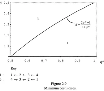
In the case o f two locations, we show that, when the capacity constraints are sufficiently tight, the risk-dominant equilibrium continues to be selected. However, as the capacity constraint is relaxed, the equilibrium switches from the risk-dominant equilibrium to states in which one location coordinates on the efficient equilibrium and the other on the risk-dominant equilibrium. W e extend the analysis to the case o f three locations and also to the case where there is inertia in strategy revision. In the three location case, the equilibrium switches from the risk-dominant equilibrium to states in which two locations coordinate on the efficient equilibrium and the other on the risk-dominant equilibrium. W e show that the results are the same when we model inertia in the strategy-adjustment process, although the equilibria are slightly more difficult to characterise. When the capacity constraint is relaxed, the equilibrium selected involves everyone playing the efficient strategy.
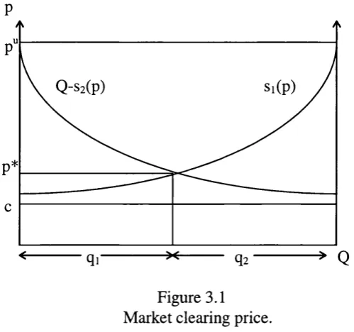
the multiple-equilibrium problem in uniform-price auctions that has been identified in the literature disappears with discrete units as long as bids are allowed in sufficiently small increments. We then present a discrete model with capacity constraints and uncertain demand. When there is no binding capacity constraint there is a unique type o f pure-strategy equilibrium under both auction formats in which the marginal price is equal to marginal cost. Both auction formats therefore result in a competitive equilibrium. When it is certain that each firm will have some residual market share, however, the expected cost is greater under a uniform-price auction. Under the uniform pricing rule there is a unique type of equilibrium in which the marginal price (and therefore the price paid for all units) is equal to the maximum permissible price. Under a discriminatory auction there is no pure-strategy equilibrium. We characterise a mixed-strategy equilibrium that holds for any distribution of the quantity up for auction.
In chapter 4, we present a model o f the Electricity Pool. Under a uniform pricing rule, the firms maximise profits by withholding base-load capacity to increase the probability that the marginal price is set by peak-load units which can be bid at much higher prices. This results in prices substantially above marginal cost.
price; 2) even if the firms could collude they are limited in the profits they can make. In fact, in our model, we show that in the monopoly outcome under a discriminatory pricing rule results in a lower cost than the stage-game, capacity-withholding equilibrium o f the uniform-price auction.
Chapter 2
Equilibrium Selection in Games.
How do players know which equilibrium to play when a game has multiple equilibria? This question has been at the heart o f much research in game theory. The focus o f attention has been the 2x2 Coordination Game such as the one given in figure 1.2 that has two Nash equilibria in pure strategies, one of which is Pareto-efficient but is riskier to play than the other. Harsanyi and Selten (1988) call the former equilibrium payoff-dominant and the latter risk-dominant. Schelling (1960) appeals to the prominence o f efficiency to suggest that agents will play for the payoff-dominant equilibrium in the expectation that other agents w ill be similarly attracted by its focal status. But Harsanyi and Selten have emphasised that such an expectation may not be well-founded. If each player optimises on the assumption that the opponent is equally likely to play either strategy, the outcome will be the risk-dominant equilibrium o f the game, which therefore also has a focal status that may outweigh that o f the payoff-dominant equilibrium.
To illustrate the idea consider again the Coordination Game o f figure 1.2. The game has two pure-strategy equilibria, e, = (s,, s,) and e^ = (s^, s^). Notice that e, is payoff-dominant while e^ is risk-dominant. There is also a mixed-strategy equilibrium where s, is played with probability 2/3. When expressed in terms o f the fraction q o f the population using strategy s,, these Nash equilibria correspond respectively to q = l, q=0 and q=2/3. W e begin by studying a specific dynamic system for which the population states q=l and q=0 are stable stationary points. Denote these stationary states by E, and respectively.
Assume that members o f the population are randomly matched each period to play this game. They adjust their choice by playing the strategy that yielded the highest expected payoff in the previous period when they are given the chance to do so. Now consider the case where q>2/3. If a revision opportunity arises, then the optimal response against the current state is to play s,. The proportion playing s, will therefore grow over time until the state where everyone plays s, is reached. The basin o f attraction o f E, is therefore (2/3, 1], since it w ill be selected from any state where q>2/3. Similarly the basin of attraction o f E^, where everyone plays s^, is [0, 2/3). A third possible stationary state (provided the population size N is infinite) is q = 2/3. At this point, no agent has an incentive to change his strategy. However, only E, and E^ are locally stable.
mutations. Once in an equilibrium, it is therefore no longer the case that the system w ill stay there forever because enough simultaneous mutations will eventually occur to move the system into the other basin o f attraction. The system therefore needs to be described in terms o f a probability distribution over the states, with much o f the time spent in or close to the two stable states when the mutation rate is small.
Kandori et al show that, when the probability o f mutation goes to zero, the distribution becomes concentrated entirely on the risk-dominant equilibrium, Ej. The reason for this is that more mutations are required to move from to E, than from E, to E^. As the mutation rate goes to zero the probability o f the first transition becomes negligible compared with the second. The time-limit o f the distribution over population states therefore puts all its mass on E^ when the mutation rate becomes vanishingly small. Following Kandori et al, equilibria that have a positive probability as the mutation rate goes to zero w ill be called long-run equilibria.
only with a subset o f the population who are close to them. He shows that a small number o f mutations concentrated together may be enough to upset the payoff-dominant equilibrium'.
Although the overwhelming consensus o f this literature is that the risk-dominant equilibrium w ill be selected, this is not always the case when local interaction is modelled. In Kandori et al, the location structure does not matter since each agent is equally likely to be matched with every other agent in the population. In models o f local interaction, agents are more likely to be matched with neighbouring players. An agent’s choice o f location is therefore important, since this will determine his or her expected payoff. Thus, if agents are given the chance, they will move to a location where they get a higher expected payoff. In E llison’s model, however, this phenomenon is absent, since agents are located at
fix ed positions around a circle and remain there. If this assumption is relaxed, a few mutations need no longer be enough to upset the payoff-dominant equilibrium because agents may m ove away from a locality in which deviant mutations have occurred in search o f a higher payoff. Similarly, the risk-dominant equilibrium may now be easier to upset since a few localised mutations may entice movement towards this locality. Ely (1995) presents a model based
on this idea in which such movement makes the long-run equilibrium Ej rather than E^.
In this chapter, we consider the consequences o f movement with the restriction that there is a capacity constraint limiting the number o f agents who can reside at each location. We begin by analysing the case where strategy^ revision is instantaneous, i.e. everybody revises their strategy each period, but the chance to move to another location only arises with some positive probability. This model is analysed with two and three locations or islands. In the two location case, it is shown that there is a range o f parameter values for which the long-run equilibria involve one island playing the efficient equilibrium and the other playing the risk-dominant one with the first island full to capacity. This extends to the three-location case, where two islands play the efficient equilibrium.
In section 2.2.3, we show that the results hold when there is inertia in strategy revision. Section 2.2.4 looks at the consequences o f relaxing the capacity constraint altogether. As in Ely (1995), the efficient equilibria are then favoured.
2.1 Stochastic Techniques.
Kandori et al (1993) & Young (1993) use a result due to Friedlin & Wentzell (1984) to characterise the stationary distribution o f a Markov chain. This enables them to analyse the behaviour o f the distribution as the mutation rate becomes vanishingly small. Using this characterisation, Kandori et al show that in the limit the stationary distribution becomes concentrated on a set o f states which they call long-run equilibria, and that these states have the property that they require the low est number o f mutations to move to from all other states taken together. Young shows that to find the long-run equilibria, it is sufficient to look at the number o f mutations required to move between the set o f equilibria rather than the set o f states. In this section, we give a brief review o f the stochastic techniques developed in these papers.
2.1.1 Friedlin & Wentzell
Consider a finite Markov chain, P, with state space S=(1,2,...,N ). A stationary distribution o f a Markov chain satisfies m=mP- It is well known that an irreducible and aperiodic Markov chain has a unique stationary distribution. For large N the problem o f solving for m becomes intractable. However, there is a
useful way o f characterising the unique stationary distribution which is sufficient for our purposes.
A z-tree, h, defined on state space S, is a set o f ordered pairs,
(/ j ) i j G S , such that each state i;^z is the initial point o f one arrow and
Then define the number u .
(/ •
h&H, ( i ^ j ) e h
N ow consider the directed graph, g, where each state i e S is the initial point o f one arrow and there is a unique loop which contains z. The set o f all possible graphs for state z is denoted .
Define the number,
r i
4
g e G , 0 ^ j ) e g
The sets H, and G, are illustrated for the case S=( 1,2,3).
^ 2 ^ 3
t 2
^ 3
can be written in terms o f u^ as follows,
i * z i ^ z
That is we can either take each i-tree, i7^= z, and add the transition i ^ z or take each z-tree and add the transition z ^ i for all i z.
Hence
i * Z i * Z
u=Pu where u=( u,
1 “ /
j
So normalising the vector u gives us the unique stationary distribution.
2.1.2 Kandori Mailath and Rob.
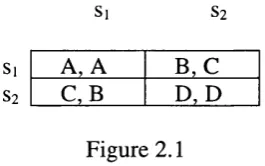
This paper looks at the consequences o f introducing ongoing mutations into an evolutionary model. The main result is that the set o f equilibria is drastically reduced in the limit as the mutation rate goes to zero. Consider a finite population that is randomly matched each period to play the 2 x 2 symmetric game o f figure 2.1.
Si S2
S] S2
A, A B ,C C ,B D .P ,
Figure 2.1
Coordination Game this will result in convergence to either the state 0 or N depending on the initial point. Without mutations the system will then remain there forever. If we now allow agents to change their strategy with some positive probability 8 independently o f each other, then the system will no longer get stuck in one o f the equilibrium states. In fact, there will be a positive probability of going from any state to any other, as any number o f simultaneous mutations can occur. We therefore have an irreducible and aperiodic Markov process, P, on state space S = (0 ,1 ,....,N ). Each transition probability, Pÿ, is a polynomial in 8. We now make use o f the characterisation o f the unique stationary distribution given in section 2.1.1.
The value u^ is constructed by taking the product o f transition probabilities along each z-tree and summing this over all z-trees. Hence u^ is also a polynomial in 8. The stationary distribution is just a normalisation o f the vector u and is given
uAe)
by n (e) = ( H |(e ),... where H ,(£ ) =
We are interested in li m |i( 8 ) . Let the low est power o f 8 in u^ be and
define L = min L . z e S ^
If L > L then > 0 as 8 ^ 0
If L = L then > f as e - > 0 where 0 < / < I
Hence the limit distribution |X = lim)Li(8) will put a positive probability on E->0
o f the lowest power. Let be the lowest power o f 8 in Pj^. W e call this the cost of the transition i- ^ j , since it is the minimum number o f mutations required for the transition. The cost o f a z-tree, h, is the minimum number o f mutations required
to move along it. This is given by c^ = ^ c.j . The low est power o f 8 in u^ will be
determined by the z-tree which has the low est cost. Thus L^= min c^.
heH^
Therefore L* will be determined by the state that has the lowest cost z-tree o f all states. So all we need to do to characterise the limit distribution is to find the state which has the lowest cost z-tree.
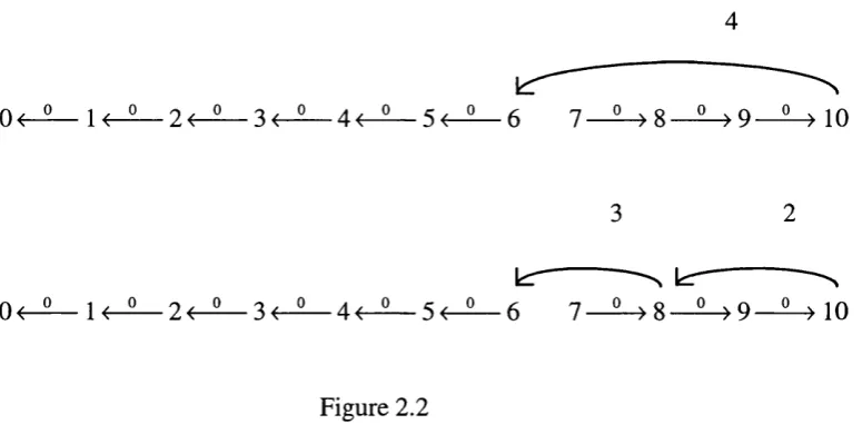
To illustrate the idea, consider the following example. A population o f 10 individuals are randomly matched to play the Coordination Game given in figure 1.2. The state o f the system at time t is given by the number o f agents playing s,, q^. Assume the dynamics are such that each period one agent revises his strategy: if seven or more agents play s,, the deterministic dynamics will move one place towards the state 10; if six or less play s,, the dynamics will move one place towards the state 0.
will move to =6. There are other ways o f moving to state 6. For example, we could have four o f the s, players and both o f the s^ players mutating. This requires six mutations. Note that in this case the smallest power o f 8 in is 2.
State 9 cannot have the minimum cost z-tree because it includes an arrow out o f state 10 which must have a positive cost. A 10-tree will not have this cost and there is a transition from 9 to 10 at zero cost. Therefore for every 9-tree there is a lower cost 10-tree. This is true for all states in the basin o f attraction o f state 10 and also for all states in the basin o f attraction o f state 0. So that leaves us with tw o candidates for minimum cost z-tree, state 0 and state 10. The minimum cost 0-tree is achieved by just enough mutations to get into its basin o f attraction.
0 < - ^ l < - ^ 2 < - ^ 3 f - ^ 4 f - ^ 5 < - ^ 6 7 — ^ 8 —^ 9 — ^ 10
Figure 2.2
Figure 2.2 illustrates that two jumps to get out o f the basin o f attraction will require more mutations than one jump since the dynamics will push back towards state 10. Similarly, the minimum cost 10-tree has a cost o f 7. Therefore
2.1.3 Young
Peyton Young goes one step further to show that we only need to consider the cost o f moving between the recurrent communication classes o f the unperturbed process. In the above example the unperturbed process is deterministic. In general the unperturbed process may follow a Markov chain, with recurrent communication classes which have the following properties: from any state x the process will move to a state which is in one o f these classes; once there the process will move between states within the class. If the perturbed process is irreducible, then the system can move between classes but this will involve a cost since mutations are required. Denote the classes by X , Xy Let n be the lowest cost o f moving from class i to j. N ow define a j-tree exactly as a z-tree but where the vertices are the indices (1,2,..., J). Let y j be the cost o f the
least cost j-tree and y (z) the cost o f the least cost z-tree. Then he shows
y (x) = y J for all x e X j. The intuition is easy to see. If we want the minimum
2.2 When Does Immigration Facilitate Efficiency.
In this section, we present a model o f local interaction with movement between locations. W e assume that agents are randomly matched with someone at the same location to play the game o f figure 2.3 in which A>C, D>B, A>D and A+B<C+D. Hence e,=(s,, s,) is the payoff-dominant equilibrium while e^ =(s^, s j is risk-dominant. The probability with which s, is played in the mixed-strategy equilibrium is q* = (D -B )/(A -C +D -B ) > 1/2.
Si S2
51 52
A, A B ,C
C ,B D ,D
Figure 2.3
Each period some agents are given the chance to move locations. We begin by looking at the case where there are two locations and strategy revision at each location is instantaneous. The analysis is then extended to the case of three locations and to the case where there is inertia in strategy revision.
2.2.1 Two Islands
However, an agent cannot move to an island that is full to capacity. If the number o f agents who wish to move to island i is greater than (N (l+d)-ni), where ni is the current number on the island, then only (N(l+d)-nj) o f them will be allowed to move. N is sufficiently large that the following set o f numbers are all integers, {N (l-d ), N (l+ d ), q*N, (l+ d )q*N , (l-d )q *N , (l-d )(l-q * )N , (l+ d )(l-q * )N } . One can think o f the following story underlying these dynamics. At the end o f each period players gather information on the proportion o f the population using each strategy on their island. With some positive probability, they also learn the proportions on the other island. At the beginning o f the next period they choose a location and strategy to use for that period. If they have no information about the other island then they stay where they are and choose the strategy that is a best reply to the proportions in the previous period. If they do learn the proportions on the other island then they will want to move if a best reply on the other island yields a higher expected payoff. If the island has spare capacity they will move and play the best reply. If it is full then they play a best reply on their current island.
The state space is
S = {(— ,--- ,«,):«] E (0,l,...,n,),n2 G (0 ,l,...,2 A -n , ),A(1 - J) <n^ < N(\ + d) } ,
rt, 2 A - « ,
where is the number playing strategy S\ on island i and ni is the number of
agents on island 1. Denote a state o f the system by s=(qi ,q2 ,n i)e S, where q, is
the proportion o f the population playing Si on islands i.
communication class. The recurrent communication classes are characterised latter.
Without mutations, the system will move to one of these classes and remain there. N ow assume that each agent mutates independently, with probability 8, with the consequence that a strategy^ is re-selected at random on their current island. This allows the system to m ove between classes and gives rise to the perturbed transition matrix where,
I N
(2.1) A=1
P^- is the ijth element o f P, the unperturbed transition Matrix.
Proposition 2.1:
P^ has a unique stationary distribution pfej andlim^^^
p (e)exists and is equal to one o f the stationary distributions o f P.
Proof:
Young (1993) shows that this is true if P^ is a ‘regular perturbation’ o f P.If P^ is a regular perturbation o f P then the following conditions must hold, i) P^ is aperiodic and irreducible
ii) l i m , _ P'u=Py
iii) P^j >0 for some 8 implies 3 r > 0 s.t. 0 X lim^^Q ^
From (2.1) conditions (ii) and (iii) are clearly satisfied. If P^j > 0 then r is
0 if Pij >0 or equal to the lowest value o f k such that c^k >0. We now show that P^
is aperiodic and irreducible. The diagonal elements o f are all positive. This is because in any state, there is a positive probability that nobody moves and that there are mutations that keep the same numbers playing each strategy on both islands. Hence is aperiodic. There is a positive probability o f going from any state to the class in which both islands coordinate on the same equilibrium. This simply requires a certain number o f mutations on each island. W e can then have any number o f agents on each island up to N (l+ d ) and for a given number of agents on each island, we can have any number playing each strategy, as there is a positive probability that nobody moves while a certain number mutate. It is therefore possible to go from any state to any other and the process is irreducible. QED.
Definition 2.1:
The set o f states in the support o flim^^^ fx(£)
will be called thelong-run equilibria.
Definition 2.2:
A k-tree, h, defined on state space S (the set o f recurrentcommunication classes), is a set o f ordered pairs, ( i ^ j ) i, j ^ S , such that each
state x ^ k is the initial point o f one arrow and from every state there is a path
which leads to k.
Let rij be the minimum number o f mutations required to go from class i to j. We know that such a number exists because P^ is irreducible. The cost o f a
k-tree is ^ r..
.
Proposition 2.2:
The long-run equilibria are the set o f states in the recurrentcommunication class which has the lowest cost k-tree.
For the proof the reader is referred to Young (1993). The intuition is clear. The long-run equilibria are the set o f states in the recurrent communication class that is easiest to flow into from all other recurrent communication classes. Hence to find the long-run equilibria we need to characterise the recurrent communication classes and the costs r^ o f moving between them and then find the class that has the lowest cost k-tree.
Recurrent communication classes.
One recurrent communication class is the set o f all states where qi =q2=0.
The basin o f attraction o f this class is {(q, , q2 ): q i< q * , q2<q* }, since best
replies wiU'^ lead both islands to the risk-dominant equilibrium. In this class the system will move between states where qi =q2=0 and ni e (N (l-d ), N(l-kd)), since agents move with a positive probability when they are indifferent and ni must lie in this range due to the capacity constraint.
N ow consider any initial condition with q i> q * and q2<q* . Best replies
will move the system towards qi =1 and q2=0. This will result in movement into island 1, since the higher payoff equilibrium is being played there. The system wül eventually move to the equilibrium state (l,0 ,N (l+ d )). Similarly the set o f states
with qi <q* and q2>q* form the basin o f attraction o f the equihbrium
(0 ,l,N (l-d )). The final possibility is for both populations to coordinate on the
payoff-dominant equilibrium. The basin o f attraction for this class is
{(qi , q2 ): q i> q * , qz>q* }, and the recurrent communication class is the set of
all states with qi=q2= l and n ie ( N ( l- d ) , N (l+ d )). The four recurrent
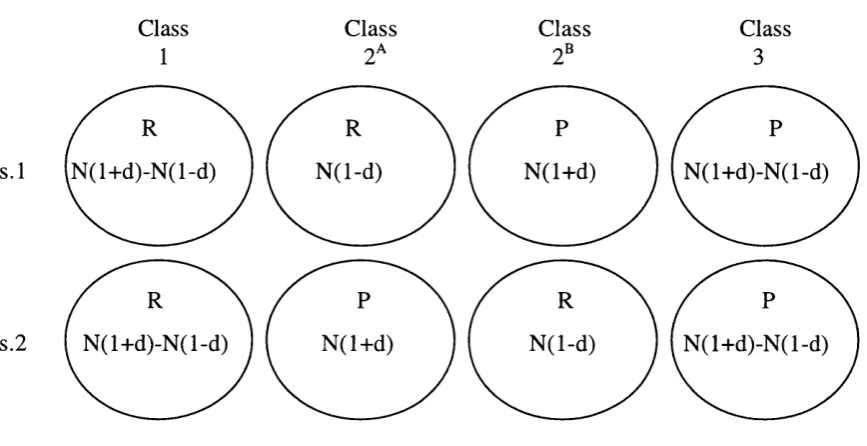
communication classes are illustrated in figure 2.4.
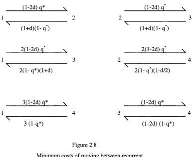
Minimum costs of moving between recurrent communication classes.
Consider the transition from class 1 to 2^. We want the minimum number o f mutations required to get into the basin o f attraction o f class two,
{(qi , q2 ): qi >q* , q2^q* }, from a state in class one, (0,0,ni). Hence we require
a proportion q* o f island 1 to mutate. N ow the less populated island 1 is, the lower the number o f mutations required to achieve this. The minimum value o f ni
is N (l-d ) so the minimum number o f mutations required is N (l-d ) q * . The dynamics will then m ove the system to the state (l,0 ,N (l+ d )). The cost o f moving back is N (l+ d ) (1-q*) since we require the system to move back to a state where qi < q* and island 1 is full to capacity.
Class
1
Class
o A
Is.l N (l+ d )-N (l-d )
Class nB
N (l-d )
Is.2 N (l+ d )-N (l-d ) N (l+ d )
Class 3
N (l+ d )
N (l-d )
N (l+ d )-N (l-d )
N (l+ d )-N (l-d )
Figure 2.4. Recurrent communication classes:
Row i o f circles illustrate the equilibrium played on island i in each o f the classes (risk-dominant, R or payoff-dominant, P), plus the range o f values of Ui that are consistent with the class.
(l-d )q A
( l + d ) ( l - q )
2 (l-d ) q* A
2 ( 1 - q )
(1-d) q' A
( l - d ) d - q )
Figure 2.5
Lemma 1:
The two location model has 4 recurrent communication classes. To find the class which has the minimum cost k-tree it is sufficient to fin d theminimum cost trees between ju st three classes, ruling out either 2^ or 2^ .
Proof:
Let rij denote the minimum cost o f the transition i ^ j .Then = r.^, r^, . = / e ( 1 , 2 , 3 ) .
Let h be a minimum cost k-tree. Adjust the tree so that at least one o f 2^
or 2® have no predecessors without changing the cost. This is easy to do since 1—>2^^ can be transferred to i —>2® (or vice versa) leaving 2^ with no predecessors. We can split the adjusted k-tree into two parts, a minimum cost k^-tree defined on the vertices (1,2,3) and 2^ added at minimum cost. It must be a minimum cost k^-tree because any adjustments which reduce the cost would also reduce the cost o f the k-tree but we started with a minimum cost k-tree. Hence we can find the minimum cost k-tree by first finding the minimum cost k^-tree and then adding a 2-state at minimum cost. This cost will be common to all k-trees and so does not need to be considered. QED
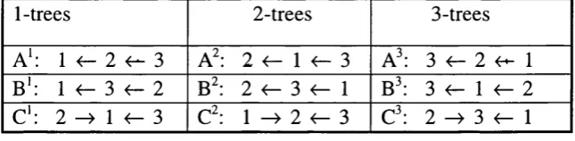
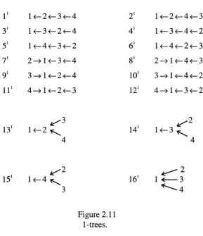
This leaves nine trees that we need to compare (3 for each communication class). These trees are illustrated in table 2.1.
1-trees 2-trees 3-trees
A ‘; 1 < - 2 3 A I 2 ^— 1 <— 3 3 2 4^ 1
B':
1 3 f - 2 2 3 1B^
3 <- 1 < - 2 C': 2 ^ 1 < - 3 C^: 1 2 « - 3 C^: 2 ^ 3 < - 1Proposition 2.3:
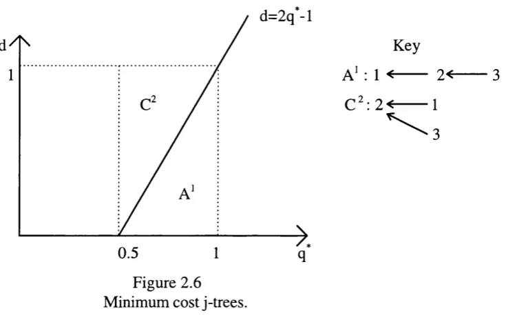
The long-run equilibria are:the set o f states in class 1 ifd < 2 q * -l,
and states 2^ and 2^ if d>2q^-l.
Proof:
From proposition 2.2, the long-run equilibria are the set o f states in the recurrent communication class which has the lowest cost k-tree. It is a simple exercise to see that the lowest cost 1-tree is A^: 1 <—2 <—3. The other two 1-trees include the transition 1 3, which has the same cost as but also include a transition from class 2 at some cost. Similarly, the lowest cost 3-tree is A^: 3 ^ 2 <— 1 as the other two 3-trees include the transition 3 <— 1, which has the same cost as A^. Finally, the lowest cost 2-tree is C^: 1 —>2<—3. The other two 2-trees include the transitions 3 —> 1 and 1 —> 3. In each case the cost is reduced by going directly to class 2.The only difference between the cost o f and A^ is in the transition
1 2
between classes 2 and 3. Since T2 3>T32 (as q * > —), C always has a lower cost.
This leaves two candidates for minimum cost k-tree, A^ and C^. The cost o f A^ is less than the cost o f if r2i<ri2. Hence class 1 has the lowest cost k-tree if
(l4-d)(l-q*) < (l-d)q* => d < 2q *-l.
If the inequality is reversed then class 2 has the minimum cost k-tree. QED. The long-run equilibria are illustrated in figure 2.6. Hence the long-run equilibria are the set o f states where everyone plays S2, the risk-dominant strategy