An Analysis of the Impact of Functional Programming Techniques on Genetic Programming

(1)

An Analysis of the Impact of

Functional Programming Techniques

on

Genetic Programming

G woing Tina Yu

A dissertation submitted in partial fulfillment o f the requirements for the degree of

D octor of Philosophy of the

U niversity of London.

Department o f Computer Science University College London

(2)

ProQuest Number: U642861

INFORMATION TO ALL USERS

The quality of this reproduction is dependent upon the quality of the copy submitted.

In the unlikely event that the author did not send a complete manuscript and there are missing pages, these will be noted. Also, if material had to be removed,

a note will indicate the deletion.

uest.

ProQuest U642861

Published by ProQuest LLC(2016). Copyright of the Dissertation is held by the Author.

This work is protected against unauthorized copying under Title 17, United States Code. Microform Edition © ProQuest LLC.

ProQuest LLC

789 East Eisenhower Parkway P.O. Box 1346

(3)

Abstract

Genetic Programming (GP) automatically generates computer programs to solve specified problems. It develops programs through the process o f a “create-test-modify” cycle which is similar to the way a human writes programs. There are various functional programming tech niques that human programmers can use to accelerate the program development process. This research investigated the applicability o f some o f the functional techniques to GP and ana lyzed their impact on GP performance.

Among many important functional techniques, three were chosen to be included in this research, due to their relevance to GP. They are polymorphism, implicit recursion and higher-order Junctions. To demonstrate their applicability, a GP system was developed with those techniques incorporated. Furthermore, a num ber o f experiments were conducted using the system. The results were then compared to those generated by other GP systems which do not support these functional features. Finally, the program search space o f the general e v e n - p a r i t y problem was analyzed to explain how these techniques impact GP performance.

(4)

Ackn o wiedgem ents

I would like to thank my supervisors, Chris Clack and Robin Hirsch, for their guidance and support. The department research student tutor, Mel Slater, has helped me out on many occa sions. 1 would like to thank him for his generous support.

Bill Langdon has been my mentor during this work. Bill introduced me to the field o f Genetic Programming at the beginning o f my Ph.D. study. Since then, he has continuously helped me with my work. This thesis has improved a great deal by his detailed comments and suggestions. I would like to thank him for his time and his patience with me.

David Fogel, Peter Angeline and John Koza have provided timely assistance and encour agement on many occasions. They have made me feel what I am doing is important. I would like to thank them for being so generous to a new comer in the field.

Evolutionary computation is a friendly field. Since the beginning o f this research, 1 have been lucky to receive support from many people. EP97 accepted my first paper, which was a great encouragement to me. Tom Westerdale has always made him self available when I needed inputs to my work. A t GP97, Nic McPhee showed keen interest in my work. I was pleasantly surprised to see that he had developed my work at GP98. During my investigation o f the GP schema theorem, Riccardo Poli has patiently answered my questions either through e-mail or in person. Peter Whigham, although he had never met me, has answered my ques tions many times through e-mail. I would like to thank them for being such good compatriots.

Ann and Paul Peterken have been my dearest English friends. They provided me a home in England during the three years o f my study. I would like to thank them for their kindness.

(5)

List of Figures

1.1 GP programs development process... 15

2.1 A derivation tree in a context-free grammar GP system ... 29

2.2 Explicit recursion versus implicit recursion ... 40

3.1 Crossover operation in a grammatically-based GP system ... 46

3.2 A derivation tree in the logic grammar GP system...47

3.3 Standard GP versus partial application program representation... 50

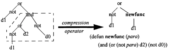
3.4 Compression operator in module acquisition...54

4.1 High-level system structure o f the functional GP system ...59

4.2 Curried format program tree for the IF-TEST-THEN-ELSE function...62

4.3 Curried format program tree with a 1 abstraction... 63

5.1 Search space versus solution space in dynamically typed G P...82

5.2 Search space versus solution space in strongly typed G P... 83

6.1 A program with nested X abstractions... 105

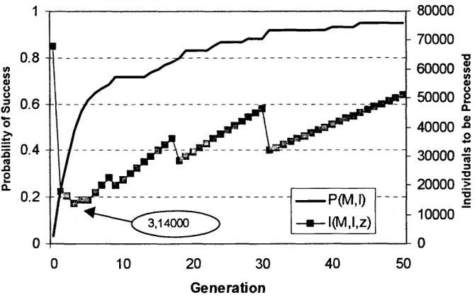
6.2 Performance curves for the general even-parity problem ... 106

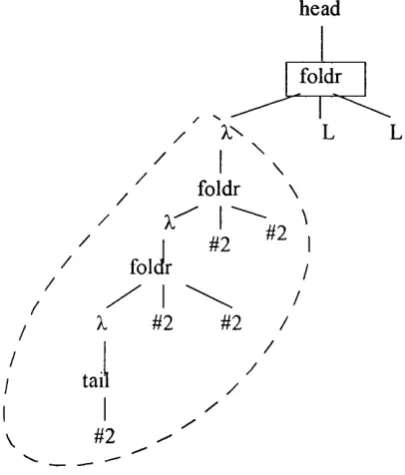
6.3 Structure abstraction grouping with foldr... 108

6.4 The evolution o f program structure grouping... 110

7.1 Structure abstraction in program tree hierarchy... 115

7.2 The foldr program tree structure...118

7.3 Program structures with 2 foldrs...119

7.4 Program structures with 1 foldr... 120

7.5 Program structures without f o l d r ... 120

(11)

7.7 Performance curves for the general e v e n - p a r i t y problem...126

A. 1 Constraint placement within stages o f evolutionary algorithms...158

A .2 Result summary charts...165

C. 1 Average fitness in the population for the artificial ant problem ...174

D. 1 Experimental results for the general e v e n - p a r i t y problem ... 177

D.2 Experimental results for the n t h program ... 179

D.3 Experimental results for the map program ... 182

(12)

List of Tables

4.1 Defaults for run-time errors in the functional GP system... 66

4.2 Examples o f functions and terminals with type in fo rm atio n ... 71

4.3 Examples o f dummy type variables instantiation... 72

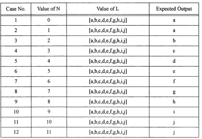
5.1 The 12 test cases for evolving nth program ... 88

5.2 The 4 categories o f nth programs with different run-time errors... 90

5.3 The 2 test cases for evolving map program... 91

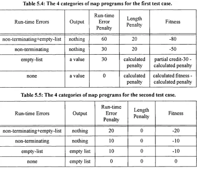
5.4 The 4 categories o f map programs for the first test case... 93

5.5 The 4 categories o f map programs for the second test case... 93

6.1 The 4 categories for general even-parity program s... 104

6.2 Performance summary for even-parity problem ... 107

6.3 Results o f 100,000 randomly generated even-parity programs 109 6.4 Generated correct general even-parity program s... I l l 6.5 Truth table for the X abstraction in the generated program s... I l l 7.1 Functions and terminals with their types... 117

7.2 16 Boolean rules found using random search... 122

7.3 foldr 11 (foldr 12 (head L) (tail L)) (tail (tail L ) ) ... 123

7.4 foldr 11 (foldr 12 (head L) (tail L)) L ... 123

7.5 foldr 11 (foldr 12 (head L) L) (tail L )... 123

7.6 foldr 11 (foldr 12 (head L) L) L ... 123

7.7 nand (foldr 11 (head L) L) (foldr 12 (head L) (tail L))... 123

7.8 nand (foldr 11 (head L) (tail L)) (foldr 12 (head L) L )... 123

(13)

7.10 nor (foldr 11 (head L) (tail L)) (foldr 12 (head L) (tail L ) ) ... 124

7.11 nor (foldr 11 (head L) L) (foldr 12 (head L) (tail L ))... 124

7.12 nor (foldr 11 (head L) (tail L)) (foldr 12 (head L) L ) ... 124

7.13 foldr 11 (fun (head L) (head L)) (tail L ) ... 124

7.14 Various techniques used to solve the e v e n - p a r i t y problem ... 125

A. 1 Classification o f constraint handling m e th o d s ... 156

A.2 Tableau o f the simple symbolic regression p r o b le m ... 162

A. 3 Summary o f experiment r e s u lts ... 164

C .l The artificial ant problem ... 173

(14)

Chapter 1 Introduction

Human computer programming involves a series of problem-solving activities. Firstly, the problem is analyzed and the parameters within the problem are defined. Secondly, a method to solve the problem is formulated. Finally, the solution is implemented and executed to solve the problem. These activities may be iterated during the programming process in order to solve the given problem.

Many modem programming techniques focus on the support o f these problem solving activities. Two popular examples are problem decomposition and contextual checking. Prob lem decomposition is a method known as “divide and conquer” ; it involves the subdivision o f a problem into smaller problems and the use o f the solutions to the smaller problems to con struct the overall solution. Contextual checking is a procedure to ensure the internal consis tency o f the program; this checking is normally carried out by an independent agent. For example, lexical/syntactic analyzers check that programs conform to the programming lan guage grammar while a type checker ensures that the types o f data and functions are consis tent with those specified by the programmers. The former technique provides guidelines to solve the problem while the later provides early warning o f program errors. Both o f them sup port a more effective program development process.

Modem functional programming languages provide a number o f unique techniques to support program development. Three o f these techniques are polymorphism, higher-order functions and implicit recursion - their details are described in Chapter 2. These techniques

(15)

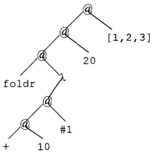
tive languages use function pointers to implement higher-order functions [Kemighan and Ritchie, 1988]. Implicit recursion is uniquely supported in functional languages through higher-order functions such as f o l d r , m ap and f i l t e r (see Section 2.3.7). It is not sup ported in other types o f programming languages. These three are powerful techniques, and have made program development an easier task [Hudak, 1989].

1.1 Genetic Programming as a Functional Programmer

The Genetic Programming (GP) [Koza, 1989, 1990, 1992, 1994a] paradigm is a problem solving method based on a computational analogy to natural evolution. In this method, com puter programs are automatically generated to solve the given problems. Initially, a popula tion o f programs is randomly created using functions and terminals appropriate to the problem domain. Each individual program is then measured in terms o f how well it solves the problem. This measure becomes the fitness o f the program. Next, the Darwinian principle o f survival o f the fittest is used to select programs for reproduction. The standard selection method is fitness-proportionate selection, where the probability o f an individual to be selected is equal to its normalized fitness value [Koza, 1992, page 97]. The programs which are selected from the current population are manipulated by genetic operations o f crossover

and mutation to generate new offspring programs. The crossover operator creates offspring using two parental programs while the mutation operator generates new offspring by altering one individual program. The generated new offspring programs constitute the new popula tion. Each individual in the new population is m easured for fitness and the process is repeated for many generations. Typically, the best program that appears in the last generation is desig nated as the result produced by GR

Consequently, there are three main phases in the GP problem solving method: 1. constructing the initial population o f computer programs;

2. evaluating each program in the population and assigning it a fitness value according to how well it solves the problem;

3. selecting “fit” programs from the current population to create new programs using genetic crossover and mutation. The new programs form a new population.

Phases 2 and 3 are iterated until the specified termination criterion is met. The best program generated at the end o f the process is the solution (or an approximate solution) to the problem.

(16)

are created based on the knowledge given about the problem (given in functions and term i nals). These programs are then tested on the problem. I f the results are not satisfactory, modi fications are made to improve the programs. This create-test-modify process is repeated until either a satisfactory solution is found or a specified condition is met.

Create

Modify j Done

Figure 1.1: GP programs development process.

Depending on the problems that GP is to solve, various issues can arise. For example the problem solution may not be able to be represented in a way which satisfies the “closure” property [Koza, 1992, page 81]. Another example is that a problem might be much more eas ily solved using recursion, yet GP has not been very successful in evolving recursive pro grams [Brave, 1996; Wang and Leung, 1996]. These issues limit the applicability o f GP. This thesis addresses these issues by introducing polymorphism, higher-order functions and implicit recursion to the GP paradigm. Extended with these techniques, GP is like a functional programmer who uses functional techniques to develop programs to solve the given problem.

Since polymorphism, higher-order functions and implicit recursion have benefited human programmers, we hypothesize that these functional programming techniques can also enhance G P’s ability in solving suitable problems. This hypothesis will be tested on the gen eral e v e n - p a r i t y problem and the map and the n t h programs.

1.2 Objectives

(17)

have enabled GP to solve these problems very efficiently. Finally, to establish guidelines for the application o f these techniques to other problems. This is partially achieved by analyzing program structures in the search space to identify how these techniques assist GP to find prob lem solutions. The guidelines are formulated accordingly.

1.3 Contributions

This research makes the following contributions:

1. It constructs a formal GP framework to evolve 1-calculus expressions.

• A single language with sufficient computation power to solve a wide variety o f prob lems is provided in GP. The language also provides a natural integration o f a module mechanism via X abstractions (see Chapter 4).

2. It demonstrates advantages provided by applying the following functional programming techniques to GP:

• polym orphism : presents the concept o f types in GP in great detail through the defini tion o f and the differentiation between untyped, dynamically typed and strongly typed

GP. The Strongly Typed Genetic Programming (STGP) [Montana, 1995] is formalized and extended to include various kinds o f type variables and higher-order function types. Moreover, the impact o f different type variables on GP search space is analyzed (see Chapter 5).

• im plicit recursion: provides recursion semantics in the evolved programs without explicit recursive calls. Previously, evolving recursive programs in GP has been diffi cult. This work not only identifies the issues that cause such a difficulty but also pro vides a solution, implicit recursion, to overcome the difficulty (see Chapter 6).

• h ig h er-o rd e r functions: supports an effective module mechanism for GP. In this approach, module creation is neither a random process nor determined in advance. Instead, it uses the knowledge (function type arguments) specified by the users in the higher-order functions to determine the m ost beneficial way to create modules. Most importantly, this work introduces a new term, structure abstraction, to describe the structure pattern emerging from the higher-order functions program representation. Structure abstraction not only enables GP to evolve a general solution to the e v e n - p a r i t y problem but also achieves greater efficiency than any other previous work (see Chapter 6).

(18)

guidelines for the application o f structure abstraction to other problems are outlined (see Chapter 7).

4. It presents a concept o f constraint handling based on the general framework o f evolu tionary algorithms (see Appendix A). This general approach provides an easy way to compare and contrast different constraint handling methods, e.g. dynamic typing versus strong typing (see Chapter 5). Moreover, the seesaw effect demonstrated in the experi ments gives a high level view o f the impact o f constraint handling on the evolutionary process, e.g. see the constraint handling for recursion error in Chapter 5.

1.4 Organization

Following this introductory chapter. Chapter 2 presents background in Genetic Algorithms, Genetic Programming and Functional Programming Languages. They are the foundation on which this work is based and from which it develops.

Chapter 3 summarizes related work. It is categorized into four areas: syntactic constraints using grammars, type constraints, modules and recursion. They are related to our work in evolving X calculus and in investigating the applicability and benefits o f the following func tional techniques to GP: polymorphism, higher-order functions and implicit recursion.

Chapter 4 describes the GP system which was developed with the mentioned functional techniques incorporated. Each component o f the system is presented, with the implementation details. The genetic algorithm used in the system and the programming language chosen to implement the system are explained. This chapter concludes with an example demonstrating the operation o f the system.

Chapter 5 presents the application o f polymorphism in GP. The concept o f types in GP is introduced through the definitions o f and differentiation between untyped, dynamically typed

and strongly typed GP. The limitation o f untyped GP in problem solving and the issues occur ring in dynamically typed GP are then summarized. This is followed by a list o f advantages that strongly typed GP can provide. The two different approaches o f strongly typed GP,

monomorphic and polymorphic GP, are then compared. This work advocates the use o f poly morphic GP, which is implemented by using three different kinds o f type variables. We ana lyze the impact o f these type variables on GP search space. Finally, two polymorphic programs are evolved to demonstrate that polymorphism has enhanced GP applicability to problems which are very difficult for GP without polymorphism to solve.

(19)

tion and its reuse is through implicit recursion. We first analyze GP issues in evolving recursive programs. Implicit recursion is then introduced as a solution to overcome these issues. We explain the 1 abstraction module mechanism and compare it with other module approaches. This program representation is then used to evolve general solutions to the e v e n - p a r i t y problem [Koza, 1992]. The experimental results show that this approach has enabled GP to find a solution with great efficiency. This chapter proposes that a program structure pattern, named "^structure abstraction’', is the cause o f the superior performance.

Chapter 7 investigates the impact o f structure abstraction on GP search. A formal defini tion o f structure abstraction is first presented. This is followed by a detailed description o f the application o f structure abstraction to the general e v e n - p a r i t y problem. The program structures and the solution structures in the search space are then analyzed. The results indi cate that structure abstraction serves as an engine o f hierarchical processing for GP search, hence allows the solution to be found very efficiently. Finally, the guidelines for the applica tion o f structure abstraction to other problems are provided.

Chapter 8 outlines our future work. Firstly, we will investigate the reason why type con strained GP is more efficient than standard GP on problems involving multiple types. Sec ondly, other forms of implicit recursion will be explored. Finally, we will apply structure abstraction to more problems.

The last chapter. Chapter 9, presents the summary and conclusion o f this thesis. This is followed by the bibliography.

In Appendix A, a concept o f constraint handling based on the general framework o f evo lutionary algorithms is presented. This approach provides an easy contrast and comparison between different constraint handling methods used in an evolutionary algorithm. Moreover, our experimental results demonstrate the importance o f constraint handling in evolutionary algorithms, for if the search space is not constrained properly, the evolution o f good solutions may be prevented.

Appendix B describes the method used to measure the performance o f the GP system in various experiments. It is essentially a brief summary o f Chapter 8 in [Koza, 1992].

Appendix C reports our experiments and their results on using a higher-order function program representation to solve the artificial ant problem [Koza, 1992].

(20)

Chapter 2 Background

The first part o f this chapter provides a brief introduction to Genetic Algorithms (GAs) [Hol land, 1992] from which GP is derived. In particular, we present the schema theorem [Holland,

1992] and the building block hypothesis [Goldberg, 1989], which were developed to explain how GAs search for problem solutions. Meanwhile, related criticisms are highlighted. This is followed by a summary o f the distinctive features o f GP and research conducted toward a GP schema theorem. The second half o f this chapter presents background knowledge in func tional programming languages, particularly in the area o f 1 calculus, polymorphism, higher- order functions and recursion. They are the functional techniques that this work applies to GP. This chapter provides background knowledge about how GP searches for problem solutions, thus enabling the analysis o f the impact o f functional techniques on GP performance.

2.1 Genetic Algorithms

GAs are search algorithms based on the mechanics o f natural selection and natural genetics. Genetic material is packed in a fixed-length string to represent an individual. A population consists o f many individuals. The natural selection scheme, survival o f the fittest, combined with two reproduction mechanisms (the traditional GA uses one-point crossover and point mutation while other GAs use different operators) are used to evolve better individuals. The GA evolutionary process uses the following 3 artificial operators to mimic natural evolution:

• Fitness-proportionate selection: Darwinian survival o f the fittest;

• One-point crossover: a sexual reproduction operator which generates offspring by inter changing sub-strings from two individuals;

(21)

These operators seem simple, yet they provide a powerful search algorithm which explores new search points with improved performance by exploiting historical information.

The schema theorem and the building block hypothesis were developed by [Holland, 1973; Holland, 1992] and [Goldberg, 1989] respectively to provide a theoretical framework for GAs. The schema theorem uses a mathematical formulation to explain why GAs are capa ble o f searching for problem solutions. This theorem is further expanded with the building block hypothesis to explain how partial solutions are carried down generation by generation to build overall solutions. However, these two works have been widely criticized recently. The details o f these two theoretical works and the related criticisms are presented in the fol lowing sections.

2.1.1 Schema Theorem

In [Holland, 1992], a schema is defined as a template describing a set o f points, from the search space o f a problem, that have certain specified similarities. Each schema is a string over an extended alphabet consisting o f the original alphabet (0 and 1) and a hash symbol (the “don’t care” symbol). For example, the schema “0##1” describes 4 similar points: “0001”, “0011”, “ 0101” and “0111”. In the conventional GA, the number o f individuals contained in the population is usually infinitesimal in comparison to the search space o f the problem. How ever, each individual in the population represents 2^ schemata, where L is the length o f the string. Consequently, the fitness-proportionate selection for reproduction, which explicitly operates only on the individuals present in the population, actually performs on a much larger number o f schemata implicitly. However, this claim has been criticized by [Macready and Wolpert, 1996].

With the fitness-proportionate selection, the expected number o f occurrences o f every schema in the next generation can be estimated. Suppose that at a given time t, there are m

individuals representing a particular schema H in the population. This is represented with the notation m(H,t). At time r+7, the expected number o f individuals representing the schema H

in the population, represented as E [ m ( H , t + 1 ) ] , is given as the following:

E[m(H,t + 1)] = (I)

m

(22)

als representing the schema to the average fitness o f the population. Put in another way, schemata with fitness values above the population average are expected to receive an increas ing number o f individuals in the next generation, while schemata with fitness values below the population average are expected to receive a decreasing number o f individuals in the next generation.

Assuming that the fitness o f a particular schema H remains above the average f(t) an amount c • / ( / ) where c is a constant, the equation can be rewritten:

+ 1)] = (1 + c) •

m{H,t)

(2)

f i t )

Only when the population is infinite and c is a stationary value, this equation represents a geo metric progression. This means that a schema with above-average fitness will appear in the next generation at an approximately exponential increasing rate over those generations. Hol land [1992] argued that this exponential increasing rate is the optimal way o f schemata pro cessing through his analysis o f the two-armed bandit problem described in the following subsection.

The Two-Armed Bandit Problem

In the two-armed bandit problem, there is a slot machine which has two arms. Furthermore, one o f the arms pays reward pj with variance and the other arm pays reward \x^ with vari ance cs\ where pj > P2- The objective is to get the most reward by playing the arm with higher reward more frequently (the arm with a pay-off p j). But how do we know which arm to play in each trial, since we have no knowledge about which arm is associated with the higher reward? Ideally, we would like to make a decision which can provide not only a good reward but also information about which is the better arm to play for the next trial. There is a trade o ff between these two wishes o f the exploration for knowledge and the exploitation o f that knowledge. Such a dilemma is a fundamental theme in adaptive systems. The two-armed ban dit problem is therefore a good candidate to study the optimal trials in any adaptive system such as GAs.

In an experiment, presume that a series o f trials have been conducted. The goal is to use the acquired knowledge to decide which is the better arm to play in the rest o f the trials. This experiment has an expected loss, L, playing the wrong arm, as the following equation:

(23)

N = total number o f trials in the experiments.

n = num ber o f trials that have been conducted on each o f the two arms with a total o f 2« trials.

q(n)= probability that the wrong decision is made after the 2n trials. Equation 3 identifies two sources o f loss:

• The first loss is a result o f choosing the wrong arm, the arm associated with the lower payoff, after performing the 2n trials. This means that we choose n wrong arms during the 2n trials and also during the rest o f the (N-2n) trials. There are a total o f

(n+(N-2n)) = (N-n) such trials.

• The second loss occurs when we select the correct arm, the arm associated with the bet ter payoff, after the 2n trials. This means that we have issued n trials choosing the wrong arm during the 2n trials with a probability o f (l-q(n)).

The objective is to allocate the N trials between the two arms so that the expected loss,

L {N ,ri), can be minimized. Holland [1973, 1992] has calculated that to allocate trials opti mally (in the sense o f minimal expected loss), an exponentially increasing number o f trials should be given to the observed better arm, i.e. the arm which receives the reward pi in the current trial.

In order to apply the result o f the two-armed bandit analysis to GAs, where multiple schemata are competing simultaneously, Holland expanded his analysis to the k-armed bandit problem. Holland [1992] demonstrated that the optimal solution to allocate the trials o f k

competing arms is similar to the solution o f the two-armed problem and argued that an expo nentially increasing number o f trials should be given to the observed best o f the k arms.

This result o f optimal allocation o f trials to the k-armed bandit can be applied to GAs by viewing the process o f GA search as a competition o f k schemata. Two schemata A and B with individual positions o, and 6, are competing with each other if for positions i =1,2..., /, at least one o f the i value has feature such that a - # #, b- # # and a - ^ b-. For example, the fol lowing four schemata are competing at locations 2 and 3:

# 0 0 # # 0 1 # # 1 0 #

# 1 1 #

(24)

the observed best schema, just as we give exponentially increasing trials to the observed best arm in the /r-armed bandit analysis.

This analysis o f the optimal allocation o f trials has been criticized by [Fogel, 1995, page 134]. First, it assumes the independent sampling o f schemata. In fact, m ost GAs employ cod ing strings such that schemata are not sampled independently [Davis, 1985]. Second, sam pling schemata in a way to minimize expected losses does not guarantee the discovery o f the global optimal solutions. Consider the two arms of a bandit, each having mean payoffs pj and P2 and each having variances o f a j and , assuming also that p j > P2 and c j « To minimize the expected loss (equation 3), all trials should be devoted to the first distribution because it has the larger mean. W hen the optimal solution is in the second distribution, it can never be discovered. For example, a schema A which represents 4 individuals each having fit ness 10 would have an average fitness o f 10. Another schema B which represents 4 individu als with fitness 0, 0, 0 and 20 respectively has an average fitness o f 5. The minimizing expected losses approach would choose to sample schema A. However, the optimal solution (with fitness 20) is described in schema B, which will not be found by sampling with the prin ciple o f minimizing expected losses. “Identifying a schema with above-average performance does not, in general, provide information about which particular complete solution, which may be described by very many schemata, has the greatest fitness. The single solution with the greatest fitness (i.e. the globally optimal solution) may be described in schemata with below-average performance. The criterion o f minimizing expected losses is quite conserva tive and may prevent successful optimization.” [Fogel, 1995].

With the assumption that the exponential increasing o f schemata with above-average fit ness from one generation to another provides the optimal way to explore the search space in mind, we are now back to the schema theorem. Notice that the schem a theorem states that the optimal schemata processing is achieved through the straightforward operation o f fitness pro portionate reproduction. Unfortunately, this selection operator doesn’t introduce any new individual to the population. If the population size is the same as the search space, this w on’t be a problem (and this GA will find a solution in generation 0 through random search). To explore new and better individuals, variation operators such as crossover and mutation are needed. These variation operators disrupt schemata during their process and will impact the schema growth from generation to generation.

(25)

crossover is performed within the defining length among the total o f /-I possible crossover locations (/ is the length o f the schema). Assume is the probability that the crossover is per formed, and the location o f crossover point is selected randomly, the probability that a schema survives from the disruption o f crossover, represented as is given in equation 4.

The inequity in equation 4 is due to the fact that crossover within the defining length o f a schema does not always disrupt the schema. For example, schema H is “ 11#####”. When crossover takes place between the first and the second positions o f two strings “ 1110101” (which schema //re p re se n ts) and “0100000”, the generated new string is “ 1100000” . The result o f the crossover does not disrupt schema / / , although the crossover takes place within the defining length o f the schema.

The next operator to consider is point mutation. The probability o f disrupting a schema H

due to mutation depends on the order o f the schema, represented in notation o(H). The order o f a schema is the number o f non-# symbols it contains. For example: “ 1#01” has order 3 while “#0#0” has order 2. Order is the number o f places where mutation can effect a schema. Assume is the probability that the mutation operation is performed and the mutation loca tion is randomly selected within an individual, the probability that a schema survives from the disruption o f mutation is the probability that all non-# symbol in the individual survive. This can be described in the following equation.

p / m ) = (1

(

3 )

Equation 6 gives the lower bound for the expected number o f individuals representing schema

H in the next generation under fitness-proportionate selection, one-point crossover and point mutation. It is the combination o f equation 1,4 and 5.

+ 1)] > -4 ^ • (1 ■ [ 1

Â 0

/ - I J

(6)

(26)

schemata with above average fitness, short defining length and small order will appear in the next generation at an exponentially increased rate, which in turn provides the best way o f schema processing, according to the analysis o f the two-armed bandit problem.

2.1.2 Building Block Hypothesis

The schema theorem perceives the operation o f GAs through the manipulation o f schemata. The schemata with short defining length, low order and high-fitness are sampled m ost favor ably because they have smaller disruption rates during crossover and mutation. In a way, GAs work by sampling these particular kind o f schemata (the building blocks), recombining, and reassembling them to form individuals o f potentially higher fitness. According to [Goldberg, 1989], the power o f GAs is due to the ability to find good building blocks and to propagate them from generation to generation at a rate close to the optimal rate. This is called the build ing block hypothesis.

Dissenting arguments against the schema theorem, two-armed bandit analysis and the building block hypothesis have been expressed a number o f times in the past and are addressed more profoundly in recent years. Since these topics are beyond the scope o f this thesis, only related works are listed below for interested readers. Salomon [1998] also pro vides a comprehensive review o f related issues.

• Both [Grefenstette and Baker, 1989] and [Muhlenbein, 1991] have criticized the schema theorem for not reflecting the real operation o f GAs.

• Altenberg [1995] also dismissed the merit o f the schema theorem in explaining GA per formance.

• Fogel and Ghozeil [1998] pointed out that the schema theorem overlooked the misallo- cation o f trials in the proeess o f stochastic effects.

• The main theoretical proof o f the incorrectness o f the two-armed bandit analysis was first offered in [Macready and Wolpert, 1996; Macready and Wolpert, 1998].

• Later, Rudolph [1997] presented a counter example to demonstrate that the fitness pro portionate selection method is not optimal in uncertain environments.

(27)

2.2 Genetic Programming

Genetic Programming (GP) [Koza, 1992] is an extension o f GAs. Similar to GAs, GP uses a central algorithm loop which applies the basic evolutionary-based genetic operators within a population o f individuals to search for solutions. The most common way used to differentiate GP from GAs is that GP uses a dynamic tree representation and the representation is inter preted as a program. In addition, there are a number o f emergent properties in GP that have distanced GP from GAs even further.

2.2.1 Genetic Programming Versus Genetic Algorithms

The following are emergent properties o f GP that have been identified by [Angeline, 1994; Altenberg, 1994a; Altenberg, 1994b; Banzhaf, Francone and Nordin, 1997].

Dynamic Tree Representation

With the variable length program tree representation, GP evolves program contents and struc tures at the same time. The search space o f GP is therefore more complicated than that o f the traditional GAs, where only the contents o f an individual are evolved. However, this property, strictly speaking, is not unique to GP. The tree representation is normally constrained to a maximum depth or a maximum number of tree nodes due to the virtual size o f a computer’s memory. In practice, the representation o f the “dynamic” tree is implemented using part o f a frxed-length bit string necessary to represent the tree. As the tree grows, more o f the bit string is used. This approach has been used by others to implement their GA work [Shaffer, 1987; Goldberg, Deb and Korb, 1990; Jefferson et al. 1992].

Complex Representation Interpretation

(28)

Syntax Preserving Crossover

The one-point crossover used in GAs is replaced with a subtree crossover in GP. This cross over operator preserves the syntax o f the programs by swapping only complete subtrees between two parent programs. Many concerns have been raised regarding to its impact on the GP evolutionary process. Supposedly, this operator should provide GP the search power to find a good problem solution. However, [O’Reilly and Oppacher, 1995] has reported the opposite results: this crossover operator seems to destroy rather than facilitate the construc tion o f problem solutions. To provide better performance, many alternative genetic operators have been proposed [O’Reilly and Oppacher, 1996; Angeline, 1997a; Chellapilla, 1997b; Harries and Smith, 1997; Poli and Langdon, 1998b].

Emergence o f Introns

A tendency o f GP program evolution is the growth o f program length, commonly known as “bloat” . Langdon and Poli [1997b] have argued convincingly that “such growth is inherent in using a fixed evaluation function with a discrete but variable length representation” . Briefly, the fixed evaluation functions quickly drive search to converge, in the sense o f concentrating the search on solutions with the same fitness as previously found solutions. In general, vari able length allows many more long representations o f a given solution than short ones o f the same solution. Consequently, the longer representations occur m ore often and representation length tends to increase.

Angeline [1998] also pointed out an obvious, yet ignored, reason o f bloat: subtree cross over promotes the recombining o f larger program structures. W hen a set o f 6 mutation opera tors is used to run three different problem experiments, Angeline showed that the program size does not grow as much as that using subtree crossover. This result is expected since 5 o f these 6 mutation operators either modify a single program point or a program link, i.e. result ing no change o f program size. The only exception is a subtree mutation which can potentially generate larger program trees. Consequently, program evolution using these 6 mutation oper ators does not cause the increase o f program size as much as that using subtree crossover.

(29)

unlike GAs where introns have to be designed into its representation [Levenick, 1991], introns in GP are emerged to its representation naturally through the dynamics o f the repre sentation.

2.2.2 Genetic Programming Schema Theorem

There are some theoretical works on defining the concept o f schem a for program trees and using them to define a schema theorem for GP [Koza, 1992; O ’Reilly and Oppacher, 1995; W higham, 1996b; Poli and Langdon, 1997; Rosea, 1997a]. Poli and Langdon [1998a] pro vided a good review o f schema definition by different researchers. Basically, there are two m ain approaches in schema definition; Non-rooted tree and Rooted tree. The following is based on their work with more detailed explanations.

Non-Rooted Tree Approach

In this approach, a schema is a non-rooted program tree. The same schema are allowed to be present multiple times within a program parse tree. Since GP program trees can have many different sizes and shapes, multiple occurrences o f the same schema can make the computa tion o f the probability o f schema disruption difficult. The formulation o f schema theorems for GP using this approach is therefore inconclusive.

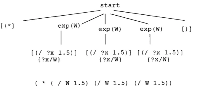
Koza [1992, page 117-118] made the first attempt to provide a schema definition for GP program trees. A schema H is represented as a set o f S-expressions. For example the schema

H = {(+ 1 x), x y )} represents all programs including at least one occurrence o f the expres sion (+ 1 x) and at least one occurrence o f (* x y ). Koza’s definition gives only the defining components o f a schema not their position, so the same schema can be instantiated in different ways, and therefore multiple times, in the same program tree. Koza didn’t provide a schema theorem for GP.

(30)

ways, and therefore multiple times, in the same program. For example the program (IF (+ 3 4) 3 4) ( - X 2)) instantiates the schema once while the program (AND (+ 3 4) (+ 3 4) (+ 3 4)

(-x y )) instantiates the schema three times because there are three ways to combine the two (+ 3 4) subtrees and one (-# #) fragment.

Based on the schema definition, the concept o f order and defining length in GP are devel oped. The order o f a schema is defined as the number o f non-# nodes in the subtrees or tree fragments contained in the schema. For example, the schema {(+ 3 4),(+ 3 4)} has order 6 and the schema {(- # #)} has order 1. The defining length is defined using two factors: the schema and its instantiation program. The defining length o f a schema is the number o f links included in the subtrees and tree fragments plus the links which connect them together in its schema instantiation program. For example, the schema {(+ 3 4),(+ 3 4)} and its instantiation program (IF (+ 3 4) (+ 3 4) (- x 2)) has defining length 4 (for schema) + 2 (for instantiation program) = 6. If a schema is instantiated in multiple programs in a population, the average number o f links to connect the schema’s subtrees for all the instantiated programs is used to calculate the defining length o f the schema.

Using these definitions o f schema, defining length and order, they developed a schema theorem for GP. In the theorem, the probability o f disrupting a schema due to crossover is not a constant but varies depending on the shape, size and the composition o f its instantiation pro grams. This is due to the fact that the defining length o f a schema depends on the way a schema is instantiated inside the programs sampling it. O ’Reilly and Oppacher argued that this variability o f disruption from generation to generation makes the propagation and the use o f building blocks (short, low-order relatively fit schemata) unattainable.

Whigham [1996b, Chapter 6] gave schema definition in his context-free grammar GP system. In his system, a program is represented as a derivation tree from a pre-defined gram mar. The crossover and mutation operators are constrained to produce only valid derivation trees. A schema is a partial derivation tree rooted in some non-terminal symbol nodes. The schemata represented in a program are a collection o f partial derivation tree (represented as production rules) organized into a single derivation tree (which represents the program). For example, consider the following derivation tree created using a context-free grammar:

and

B

(31)

s ::= andBB;

B ::= x;

B ::= y;

The program tree in Figure 2.1 can be created using the following derivation steps:

S

=>

andBB

=>

andxB

=>

andxx

Meanwhile, the following schemata are represented in this derivation tree associated with these steps:

=>

, B ^

, -S' =>

andBB, S

=>

andxB, S

=>

andBx, S

=>

andxx, B =>x

This definition o f schema doesn’t require a special symbol for d o n ’t care since every non-ter minal {S and B in this example) in a partial derivation tree implicitly represents all legal strings that can be derived from the non-terminals. Also, a schema can appear multiple times in the same program since a schema derivation tree can be extended by applying one or more of the pre-defined grammar rules. For example, the schema ^ => x is present twice in the program derivation tree. This is due to the absence o f position information in the schema def inition.

W higham's definition o f schema leads to a simple equation for crossover and mutation disruption o f schemata without the need o f defining length and order. However, as with that defined by O ’Reilly and Oppacher, the disruption probabilities vary depending on the size o f the derivation trees which the schema represents. To formulate his schema theorem, Whigham used the average disruption probabilities for all programs which a schema repre sents. This GP schema theorem differs from the one obtained by O ’Reilly and Oppacher as the concept o f schema is different. Whigham didn’t draw any conclusion related to the build ing block hypothesis.

Rooted Trees Approach

In this approach, a schema is a rooted program tree or tree fragment. With this position restriction, a schema can only be instantiated at most once within a program tree. The study o f the propagation o f the components o f the schema in the population is equivalent to analyzing the way the number o f programs sampling the schema changes over time.

(32)

and terminals specified in the schema. The above schema example has order 2. His schema theorem doesn’t use the concept o f defining length. Instead, the disruption o f a schema due to crossover is the summation o f the disruption o f all programs in the population that the schema represents. As an example, if there are 3 programs: (+ x x ), (+ ( -y I) x) and f+ f - x y j x j in the population which match the schema H, the disruption rate for the schema is the summation o f the disruption o f the three tree programs. The disruption o f each program depends on 1) the size o f the program, 2) its fitness and 3) the order o f the schema represented. Rosea didn’t provide conclusion regarding to building block hypothesis from his schema theorem.

Poli and Langdon [1997] defines a schema as a rooted tree fi'agment whose don’t care symbol (“ =”) can only be matched by a single function or terminal. This makes a schema / / represents only those programs which has the same shape as H and which have the same labels for the non-= nodes. The number o f non-= symbols is called the order o f a schema H,

while the total number o f nodes in the schema is called the length N(H) o f the schema. The number o f links in the minimum subtree including all the non-= symbols within a schema H

is called the defining length L(H) o f the schema. For example, the schema (+ (I = = ) x) has order 3 and defining length 2.

Using the concept o f order, length and defining length. Poli and Langdon formulated a schema theorem for a GP system using point mutation and one-point crossover. Point m uta tion replaces a function in a tree with another function with the same arity or replaces a term i nal with another terminal. One-point crossover works by selecting a common crossover point (the same position counting from the root o f the tree) in the parent programs and then swap ping the corresponding subtrees like the standard crossover. They have used the defined schema theorem to analyze the disruption o f two groups o f schemata: schemata representing programs with the same shape and size and schemata representing programs with different shape and size. The results indicate that these two groups o f schemata interact with each other during GP run to optimize program structure and contents. According to their study, two con jectures have been made:

• During the early stage o f GP run, the schema disruption rate is very high. The effect o f fitness-proportional selection is counteracted by the crossover disruption.

• In the absence o f mutation, after a while the population would start converging and the diversity o f program shapes and sizes would decrease. During this phase competing schemata normally have the same size and shape, which is very much like GAs.

There-1. R osea didn’t use a “don’t care” symbol since a schem a is a rooted and contiguous tree. A ll

(33)

fore, during this stage o f GP run schemata with above average fitness, low order and short defining length (building blocks) would have a low disruption probability.

The purpose o f formulating a schema theorem for GP is to provide an understanding o f how GP searches for problem solutions. Yet, as the validity o f the GA schema theorem is criti cized, the usefulness o f GP schema theorem is also under attack. In December o f 1997, a heated debate went on the genetic programming list [GP-List, 1997] about the existence o f building block, schema interpretation and the performance o f crossover versus mutation. In fact, using a different approach, an enumeration o f the program search space, [Langdon and Poli 1998a] has concluded that there is no building block in the artificial ant problem. Further more, they also demonstrated that the ability o f GP to use building blocks to compose prob lem solutions is not exhibited in the e v e n - p a r i t y problem [Langdon and Poli, 1998b]. We have used a similar approach to investigate the impact o f a higher-order function program representation on the GP search process. This work will be described in Chapter 7.

2.3 Functional Programming Languages

This section summaries functional programming languages work which is related to this research. The X calculus is presented first. This is followed by an overview o f types and poly morphism. A polymorphic X calculus is then given. Finally, two functional programming lan guages features, higher-order functions and recursion, are described at the end o f this section.

2.3.1 Lambda Calculus

The X calculus [Church, 1932-1933; Church, 1941] is usually regarded as the first functional language, although it was certainly not thought o f as programming language at the time, given that there were no computers on which to run the programs [Hudak, 1989]. Modem functional languages can be thought o f as the X calculus (in various forms) with a lot o f syntactic sugar.

X expressions are expressions in the 1 calculus. The abstract syntax o f the untyped X

expressions is as the following:

e : : = c built-in function or constant

I X identifier

I 0 2 application o f one expression to another I À X . e X abstraction

(34)

constants, for example +. This extended version is therefore chosen as it represents m odem functional languages more closely.

Expressions o f the form X x . e are called X abstractions which represent function defini tion. Expressions o f the form 6 2 are called applications which represent the application o f an expression to another expression. By convention, application is left-associative, so that

(e^ 6 2 6 3) is the same a s ( ( e i 6 2) 6 3). The following gives some examples o f X expressions:

a

+

1

b

(X X . + 1 x )

2.3.2 The Operational Semantics of the Lambda Calculus

This section provides the “calculation” part o f the X calculus: four conversion rules which describe how one X expression is converted into another. The operation o f substitution o f the expression M for the free variable x in the expression E, denoted as E[M/x], is first explained since it is used by three o f the four conversion rules.

The set o f free variables o f a X expression E, which is represented in notion Jv(E), is defined by the following rules:

/v ( c ) = { } = { ^ )

p ( \ x e ) = f v ( e ) - { x )

A variable x is free in E i î f x g f v { E ) .

Substitution with the expression M o f every free variable x i n a X expression E (denoted

E [M/x] ) is defined inductively by: c [M /x] = c

X [M /x] = M

(6] €2) [M /x] = e i[M /x ] 6 2[M /x] (Xx. e) [M /x] = Xx. e

(35)

The last rule is the m ost complicated one. It deals with name conflict and resolves it by m ak ing a name change. The following example demonstrates the application o f this last rule;

( &y . + X y) [ y / x ] - > ( I z . + x z ) [ y / x ] -> X z , + y z Now the terminologies are clear, the four conversion rules can be presented:

a -c o n v e rsio n : Xx. e <-> ^y. e[y/x], i f y ^ y v ( e ) P -conversion; (A,x. e)M <-> e[M /x]

r|-c o n v e rsio n : (A,x. e x ) <-> e, i f x ^ f v ( e )

0 -co n version: e v a l u a t i o n o f b u i l t - i n f u n c t i o n s The following gives examples o f the application o f these conversion rules:

(Xx. + x l )

A

(Xy. + y l )

(A.X. + X 1) 6 ( + 6 1)

{ X x . +

1

X) a . (+ 1 )

+ 1 2 è 3

Note that these four are conversion rules which allow the conversion to happen in either direction. When these rules are restricted to happen in one direction, these conversion rules are called reduction rules: a-reduction, p-reduction, T]-reduction and 5-reduction. A X expres sion can be reduced to another one by applying one o f the four reduction rules.

R e d u c tio n O r d e r

A X expression is in normal form if it can not be reduced further using p or rj rules. There are some X expressions which do not have normal form, such as:

(Xx. (X X) ) (Xx. (X X) )

where the only possible reduction leads to an identical term, thus the reduction process is non terminating.

Furthermore, some X expressions may or may not reach normal forms depending on the reduction order. For example, consider the following X expression:

(Xx.

3 ) (D D) w h e r e D i s

(Xx.

x x)

(36)

The Church-Rosser Theorem I [Church and Rosser, 1936] provides an answer for this question:

I f

62, then there exists an expression e, such that e^-^ e and

^2 ^ ^ •

Corollary:

No lambda expression can be converted to two distinct normal forms.

Informally, the corollary says that all reduction sequences which terminate will result in the same normal form. The next question is which reduction order is mostly likely to terminate and to find the normal form?

The Church-Rosser Theorem II [Church and Rosser, 1936] provides an answer for this question:

I f e Y

^2'

^2

normal form, then there exists a normal order reduction

from ej to

These two Theorems promise that there is at most one possible result and normal order reduc tion will find it if it exists. So, what is normal order reduction?

A normal order reduction is a sequential reduction in which, where there is more than one reducible expression (called a redex), the leftmost outermost one is chosen first. In con trast, an applicative order reduction is a sequential reduction in which the leftmost innermost

redex is reduced first. In the above example ( ( X,x. 3 ) ( D D)), normal-order reduces the Ix - redex first while the applicative-order would reduce the ( D D ) -redex first. Intuitively, nor mal- order performs reduction on the body o f a function first while applicative order performs reduction on the argument o f a function first. In this example, normal order reduction pro duces a result while applicative order reduction will loop forever.

2.3.3 Typed Lambda Calculus

To introduce types into the 1 calculus, the type language to be used has to be defined:

a : : = X basic type

I -> ( ? 2 function type

(37)

to value o f 0 2- Thus, the type o f application ( ^ 1 ' ^ ^ 2 ' ) is 0 2. M odifying the X calculus this way, a typed X calculus can be derived;

e : : = built-in fonction and constant

I identifier

I ( ^ ^ ^ application o f one expression to another

I (A, X*' . abstraction

The typed conversion rules are as the following:

T y p e d -a-c o n v ersio n : (Ax^' .e^) <-> /x ^ ' ]), i f ^

T yped-P -conversion: ((A x^' ) <-> /x ^ ' ].

T y p ed -r|-conversion: (Ax^' .e^ x ^ ' ) <-> e*^, i f x '^ '^ / v ( e ^ ) . Typed-Ô -conversion: e v a l u a t i o n o f b u i l t - i n f u n c t i o n s

The typed A calculus supports a type system which is like that used in monomorphic typed languages. Modern functional languages do better than this by supporting polymorphism. The next section introduces the concept o f polymorphism. A typed A calculus which supports polymorphism will be discussed in Section 2.3.5.

2.3.4 Types and Polymorphism

Static Versus Dynamic Versus Strong Typing

In programming languages, static typing means that the type o f every expression can be deter mined by static program analysis. This also means that before a program is executed, the type o f every expression is known. By contrast, dynamic typing doesn’t care about the type o f an expression until program execution time. Dynamically typed languages use a run-time type checker and a run-time error handler to either report or repair type errors. Static typing is a desirable feature because it allows type errors to be detected at compile time, hence provides greater execution-time efficiency.

(38)

[Cardelli and Wegner, 1985]. For example, they exclude generic procedures, such as sorting, that represent algorithms which are applicable to a range o f types.

Strong typing relaxes the restriction by allowing the exact type o f an expression to be unknown at program compiling time. However, all expressions have to be type consistent. A program that is type consistent at compile time is guaranteed to be executed without run-time type errors. Note that every statically typed language is strongly typed, but the reverse is not necessarily true.

Kinds of Polymorphism

Strong typing can be implemented in programming languages in two different ways. Conven tional typed languages, such as Pascal, are based on the idea that arguments o f functions and procedures have an unique type. Such languages are called monomorphic languages. By con trast, languages allow functions and variables to have m ore than one type.

Cardelli and Wegner [1985] have classified polymorphism as the following:

Polym orphism

.{param etric

umversaU

[

inclusion

a d

[ coercion

Universally polymorphic functions work on a large number o f types (all the types have a given common structure), whereas ad-hoc polymorphic functions only work on a finite set o f different and potentially unrelated types. With universal polymorphism, a polymorphic func tion would operate on arguments o f many types. However, this is not always true in ad-hoc polymorphism. An ad-hoc polymorphic function can be viewed as a small set o f monomor phic functions and the set can contain only one element. In terms o f implementation, a univer sally polymorphic function executes the same code for arguments o f any admissible types, whereas an ad-hoc polymorphic fimction may execute different code for different type o f argument.

An Analysis of the Impact of Functional Programming Techniques on Genetic Programming