Photovoltaic Cell and Module I-V Characteristic
Approximation Using Bézier Curves
Roland Szabo 1 and Aurel Gontean *
1 Applied Electronics Department, Politehnica University Timisoara, Timisoara 300006, Romania; [email protected] (R.S.); [email protected] (A.G.)
* Correspondence: [email protected]; Tel.: +40-745-121-383
Abstract: The aim of this work is to introduce new ways to model the I-V characteristic of a PV cell or PV module using straight lines and Bézier curves. This is a complete novel approach, Bézier curves being previously used mainly for computer graphics. The I-V characteristic is divided in three sections, modeled with lines and a quadratic Bézier curve in the first case and with three cubic Bézier curves in the second case. The result proves to be accurate and relies on the fundamental points usually present in the PV cell datasheets: 𝑉𝑜𝑐 (the open circuit voltage), 𝐼𝑠𝑐 (the short circuit current), 𝑉𝑚𝑝 (the maximum power corresponding voltage) and 𝐼𝑚𝑝 (the maximum power corresponding current) and the parasitic resistances 𝑅𝑠ℎ0 (shunt resistance at 𝐼𝑠𝑐) and 𝑅𝑠0 (series resistance at 𝑉𝑜𝑐). The proposed algorithm completely defines all the implied control points and the error is analyzed. The temperature and irradiance influence is also analyzed. The model is also compared using the least squares fitting method. The final validation shows how to use Bézier cubic curves to accurately represent the I-V curves of an extensive range of PV cells and arrays.
Keywords: PV cell; I-V characteristic; model; simulation; interpolation; Bézier curve; control points; least squares fitting method
1. Introduction
The forecast of the total PV installs, offered by Bloomberg New Energy Finance (BNEF) predicts an optimistic growth at 111 GW in 2018, rising to 121 GW in 2019, along with a polysilicon factory grow boom and module prices drop to US$0.30/W [1], [2]. This robust growth explains the high interest in PV research, modeling and simulation – along with design and development of PV equipment.
The electrical characteristics of the PV cell and PV modules have been of interest for several decades, and different models have been proposed. Phang and Chan [3] were among the first to propose a solution for PV cell parameter extraction. Garrido-Alzar [4] uses a double exponential model to extract the PV cell parameters using the experimental I-V curve. Villalva et al. [5] developed an algorithm to find the parameters defining the I-V characteristic for the single diode model of a PV cell, using the Newton-Raphson method and imposing a minimum error threshold for the maximum power point. Babu and Gurjar [6] introduce a simplified two-diode model for the PV module, while Cubas et al. [7] used the Lambert W-Function for finding the solar panel equivalent circuit parameters and they also proposed an LTSpice model according to their findings. Temperature influence is studied by Chander et al. [8]. Ishaque and Salam [9] use differential evolution to find the PV modules parameters.
Franzitta et al. provide extensive studies of the most widely used models both in single diode case [10] and for the double-diode version [11], introducing a criterion for rating the accuracy and usability of the analyzed models. In our previous paper [12], we proposed a complete SPICE model including all the parameters variation and selfheating. In a recent work, Cuce et al. [13] claim a good accuracy for their electrical model for a PV module and they also discuss energy and exergy efficiency as a reliable substitute for the fill factor. All the aforementioned works use an electrical model to describe the behavior of the circuit and rely on a specific circuit to generate the I-V characteristic of the PV cell or module.
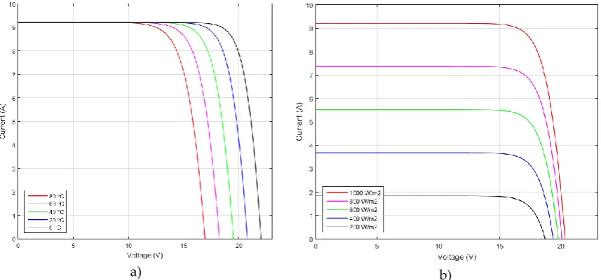
This paper introduces a new approach. This time, the cell or module are not involved at the electrical level, being defined by just the specific points 𝑃𝑠𝑐, 𝑃𝑚𝑝, 𝑃𝑜𝑐 and by the parallel and series resistances 𝑅𝑠ℎ0 and 𝑅𝑠0, specified at 𝐼𝑠𝑐 and 𝑉𝑜𝑐, respectively. Carefully inspection of the typical I-V characteristic of the PV module or PV cell (Figure 1a and 1b) shows a similar pattern in all curves. Our aim was to find a way to model it using smooth curves and datasheet information currently available.
a) b)
Figure 1. Typical PV module I-V characteristics, with 30 cells connected in series. a) at different temperatures (0 - 80 °C). b) At different irradiances (200 – 1000 W/m2).
Bernstein polynomials have been studied since the beginning of the 20th century and they form the foundation for Bézier curves [14]. The core applications for graphics came first in 1959 when the French mathematician Paul de Casteljau developed an algorithm able to evaluate a family of specific curves at Citroën. In 1962 the French engineer Pierre Bézier also used them to design automobile bodies at Renault and afterwards they got wide acceptance [15].
Bézier curves are largely used in computer graphics [16, 17] and also in time domain for smoothing the trajectory of the robotic arms, for an accurate gluing or welding path or for trajectory generation [18]. Further development for shape representation is proposed by Jalba et al. [19].
The current proposal analyses the use of Bézier curves [20] in order to accurately represent the I-V characteristic of a PV cell or module. A complete mathematical solution is provided, separately validated for a PV cell and a PV module and the error is analyzed. The results are also studied for different temperature and irradiances and finally compared with the ones offered by the least squares fitting method. In depth analysis of Bézier cubic curves fitting for 18 PV arrays and cells (from various manufacturers and different technologies) is also performed.
2. Definition of the Bézier Curves
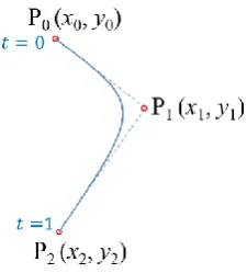
A quadratic Bézier curve (Figure 2) can be specified by three control points [15]: the curve goes through the ends 𝑃0 and 𝑃2 and approximates 𝑃1.
Figure 2. A quadratic Bézier curve representation. 𝑃0 and 𝑃2 are the end points, the control point 𝑃1 is
approximated and the curve is tangent to ̅̅̅̅̅̅𝑃0𝑃1 and ̅̅̅̅̅̅𝑃2𝑃1 segments at 𝑃0 and 𝑃2 respectively.
The curve equation is as follows [20]:
𝐵2(𝑡) = (1 − 𝑡)2𝑃
0+ 2𝑡(1 − 𝑡)𝑃1+ 𝑡2𝑃2 (1)
where 𝑡 varies between 0 and 1. Equation (1) can be expressed for the 𝑥 and 𝑦 coordinates:
{𝑥(𝑡) = (1 − 𝑡) 2𝑥
0+ 2𝑡(1 − 𝑡)𝑥1+ 𝑡2𝑥2 𝑦(𝑡) = (1 − 𝑡)2𝑦
0+ 2𝑡(1 − 𝑡)𝑦1+ 𝑡2𝑦2
(2)
The derivative of (1) is:
𝐵2′(𝑡) = 2(1 − 𝑡)(𝑃
1− 𝑃0) + 2𝑡(𝑃2− 𝑃1) (3)
At the end points, (3) becomes (4):
{𝐵2 ′(𝑡)|
𝑡=0= 2𝑃1− 2𝑃0 𝐵2′(𝑡)|
𝑡=1= 2𝑃2− 2𝑃1 (4)
A cubic Bézier curve (Figure 3) can be specified by four control points [15]: the curve goes through the ends 𝑃0 and 𝑃3 and approximates 𝑃1 and 𝑃2. The analytical expression of the curve is a cubic polynomial. The curve is tangent at 𝑃0 to 𝑃̅̅̅̅̅̅0𝑃1 and at 𝑃3 to 𝑃̅̅̅̅̅̅3𝑃2.
The equation for the Bézier cubic curve is [20]:
𝐵3(𝑡) = (1 − 𝑡)3𝑃0+ 3𝑡(1 − 𝑡)2𝑃1+ 3𝑡2(1 − 𝑡)𝑃2+ 𝑡3𝑃3 (5)
The previous equation can be expressed for the 𝑥 and 𝑦 coordinates:
{𝑥(𝑡) = (1 − 𝑡) 3𝑥
0+ 3𝑡(1 − 𝑡)2𝑥1+ 3𝑡2(1 − 𝑡)𝑥2+ 𝑡3𝑥3 𝑦(𝑡) = (1 − 𝑡)3𝑦
0+ 3𝑡(1 − 𝑡)2𝑦1+ 3𝑡2(1 − 𝑡)𝑦2+ 𝑡3𝑦3
(6)
The derivative of (5) is:
𝐵3′(𝑡) = 3(1 − 𝑡)2(𝑃
1− 𝑃0) + 6𝑡(1 − 𝑡)(𝑃2− 𝑃1) + 3𝑡2(𝑃3− 𝑃2) (7)
At the end points, (7) becomes (8):
{𝐵3 ′(𝑡)|
𝑡=0= 3𝑃1− 3𝑃0 𝐵3′(𝑡)|
Figure 3. A cubic Bézier curve representation. 𝑃0 and 𝑃3 are the end points, the control points 𝑃1 and
𝑃2 are approximated and the curve is tangent to 𝑃̅̅̅̅̅̅0𝑃1 and ̅̅̅̅̅̅𝑃2𝑃1 segments at 𝑃0 and 𝑃3 respectively.
3. Materials and Methods
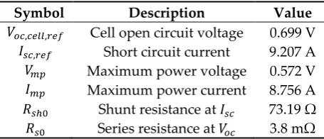
The first PV cell used in our work is a high efficiency, silicon monocrystalline 156 x 156 mm2 cell [21] and has the main characteristics summarized in Table 1.
Table 1. PV Cell main specifications on STC (1000W/m2, AM 1.5, 25°C).
Symbol Description Value
𝑉𝑜𝑐,𝑐𝑒𝑙𝑙,𝑟𝑒𝑓 Cell open circuit voltage 0.699 V 𝐼𝑠𝑐,𝑟𝑒𝑓 Short circuit current 9.207 A 𝑉𝑚𝑝 Maximum power voltage 0.572 V 𝐼𝑚𝑝 Maximum power current 8.756 A 𝑅𝑠ℎ0 Shunt resistance at 𝐼𝑠𝑐 73.19 Ω
𝑅𝑠0 Series resistance at 𝑉𝑜𝑐 3.8 mΩ
The MSMD290AS-36_EU Monocrystalline PV module [22] is well documented and studied by Cubas et al. [6]. Its main electrical data is listed in Table 2 and this information will be used in Section 4.4 to evaluate the influence of the temperature and irradiance to our Bézier curves based model.
Table 2. MSMD290AS-36_EU Module main specifications on STC (1000W/m2, AM 1.5, 25°C).
Symbol Description Value
𝑉𝑜𝑐,𝑚𝑜𝑑𝑢𝑙𝑒,𝑟𝑒𝑓 Cell open circuit voltage 44.68 V
𝐼𝑠𝑐,𝑟𝑒𝑓 Short circuit current 8.24 A
𝑉𝑚𝑝 Maximum power voltage 37.66 V
𝐼𝑚𝑝 Maximum power current 7.70 A
𝑅𝑠ℎ0 Shunt resistance at 𝐼𝑠𝑐 316 Ω
𝑅𝑠0 Series resistance at 𝑉𝑜𝑐 130 mΩ 𝑘𝐼 Current temperature coefficient 3.296 mA/K 𝑘𝑉 Voltage temperature coefficient -146.256 mV/K
𝑛𝑠 Number of series cell 72
4. Results
It must be stressed out that all the physical actual values involved in sections 4.1, 4.2 and 4.3 are specified at 25°C, being reference values. The irradiance is also standard (1000 W⁄m2). As it will be demonstrated in section 4.4., the same method is suitable for different temperatures and irradiances.
4.1. I-V Characteristic approximation with two segments and a quadratic Bézier Curve
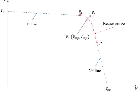
The first approximation implies five control points: 𝑃𝑠𝑐(0, 𝐼𝑠𝑐), 𝑃𝑎(𝑥𝑎, 𝑦𝑎), 𝑃𝑏(𝑥𝑏, 𝑦𝑏), 𝑃𝑐(𝑥𝑐, 𝑦𝑐) and 𝑃𝑜𝑐(𝑉𝑜𝑐, 0) and is made of two segment lines 𝐼̅̅̅̅̅̅𝑠𝑐𝑃𝑎 and 𝑃̅̅̅̅̅̅̅𝑏𝑉𝑜𝑐 and one quadratic Bézier curve defined by the endpoints 𝑃𝑎 and 𝑃𝑏 and the control point 𝑃𝑐 (figure 4).
Figure 4. Projected PV cell I-V characteristic approximation with two straight line segments and one quadratic Bézier curve.
It has already been proven [3] that the slopes of the lines can be written as (9) and (10):
𝑑𝐼 𝑑𝑉|𝑉=0
= − 1
𝑅𝑠ℎ0 (9)
𝑑𝐼 𝑑𝑉|𝑉=𝑉𝑜𝑐
= − 1
𝑅𝑠0 (10)
Thus, the equation for first line is (11):
𝐼 = 𝐼𝑠𝑐− 𝑉
𝑅𝑠ℎ0 (11)
By choosing 𝑥𝑎 in the linear region (eg 0.6𝑉𝑜𝑐), one can find 𝑦𝑎 from the above equation, so 𝑃𝑎 is completely defined.
For the second line, the next equation is valid (12):
𝐼 =𝑉𝑜𝑐− 𝑉
𝑅𝑠0 (12)
The 𝑃𝑐(𝑉𝑐, 𝐼𝑐) control point has therefore the coordinates defined by (13):
(𝑥𝑐 = 𝑉𝑐=𝑉𝑜𝑐𝑅𝑠ℎ0− 𝐼𝑠𝑐𝑅𝑠ℎ0𝑅𝑠0
𝑅𝑠ℎ0− 𝑅𝑠0 , 𝑦𝑐 = 𝐼𝑐 =
𝐼𝑠𝑐𝑅𝑠ℎ0− 𝑉𝑜𝑐
For 𝑥𝑏, it must be emphasized that its position is on the end of the curve, a realistic value being 0.9𝑉𝑜𝑐. The maximum power point is positioned on the second curve, so solving (14) gives 𝑡𝑚𝑝:
𝑡𝑚𝑝2 (𝑥
𝑎+ 𝑥𝑏− 2𝑥𝑐) + 2𝑡𝑚𝑝(𝑥𝑐− 𝑥𝑎) + 𝑥𝑎− 𝑉𝑚𝑝 = 0 (14)
Replacing the positive solution for 𝑡𝑚𝑝 in (2) yields 𝑦𝑏 as in (15):
𝑦𝑏 =(2𝑡𝑚𝑝− 𝑡𝑚𝑝 2 − 1)𝑦
𝑎+ 2𝑡𝑚𝑝(𝑡𝑚𝑝− 1)𝑦𝑐+ 𝐼𝑚𝑝
𝑡𝑚𝑝2 (15)
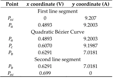
Now all the control points of the plot are completely defined. The results are summarized in Table 3. The application code written for the coordinate finding can be found here: http://tess.upt.ro.
Table 3. The control point coordinates when using two lines and one quadratic Bézier curve.
Point 𝒙 coordinate (V) 𝒚 coordinate (A) First line segment
𝑃𝑠𝑐 0 9.207
𝑃𝑎 0.4893 9.2003
Quadratic Bézier Curve
𝑃𝑎 0.4893 9.2003
𝑃𝑐 0.6070 9.1987
𝑃𝑏 0.6291 7.0181
Second line segment
𝑃𝑏 0.6291 7.0181
𝑃𝑜𝑐 0.699 0
The final plot is represented in Figure 5, where one can observe an excellent correspondence between the actual PV cell I-V characteristic, represented with black dots and the 𝑃̅̅̅̅̅̅̅𝑠𝑐𝑃𝑎 segment (blue line), a fair correlation for the second range, approximated by the Bézier quadratic curve (red line) and some modest results in the third region (magenta line).
The same conclusion arises from Figure 6, where the relative error has been plotted. It is worth mentioning that although the relative error is quite high above 0.64 V (0.92𝑉𝑜𝑐), the absolute error is in fact less than 0.7 A in a region where the cell normally should not operate.
Figure 6. Approximation errors are high over 0.64 V.
Looking for a more accurate model is the reason we came up with the second scenario, where the I-V characteristic is entirely modeled with cubic Bézier curves.
4.2. I-V Characteristic approximation with three cubic Bézier curves
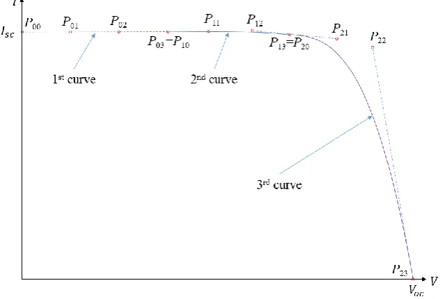
In order to have a general solution, we analyzed the case where all three regions are covered with cubic Bézier curves. This implies 12 control points (Figure 7), i.e. 24 coordinates to be found.
Figure 7. Projected PV cell I-V characteristic approximation with three cubic Bézier curves.
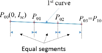
evenly arranged, with 𝑗 = {1,2}; 𝑘 = {1,2,3}. This leads to 𝑃01𝑥 =𝑃03𝑥 3
⁄ and 𝑃02𝑥=2𝑃03𝑥 3
⁄ . For the y
coordinates, 𝑃0𝑘𝑦= 𝐼𝑠𝑐−𝑃0𝑘𝑥 𝑅 𝑠ℎ0
⁄ , with 𝑘 = {1,2,3}. Now the first curve is completely defined.
Figure 8. First Bézier curve with the associated control points. The slope is exaggerated for a better understanding.
The second curve (Figure 7) is described by the control points 𝑃10= 𝑃03, 𝑃11, 𝑃12 and 𝑃13. We observed that 𝑃13𝑥 = 0.75𝑉𝑜𝑐 offers a very good fit of the curve for this type of PV cell. With the same evenly arrangement for the x coordinates, 𝑃1𝑘𝑥= 𝑃10𝑥+𝑘(𝑃13𝑥− 𝑃10𝑥)
3
⁄ , with 𝑘 = {1,2}. 𝑃11is also
located in the linear region of the I-V curve, so 𝑃11𝑦= 𝑃03𝑦−𝑃11𝑥⁄𝑅𝑠ℎ0. This leaves 𝑃12𝑦 and 𝑃13𝑦 as unknowns at this stage.
The third curve (Figure 7) is described by the control points 𝑃20= 𝑃13, 𝑃21, 𝑃22 and 𝑃23(𝑉𝑜𝑐, 0). Using the same assumptions as for the second curve, 𝑃2𝑘𝑥= 𝑃20𝑥+𝑘(𝑃23𝑥− 𝑃20𝑥)⁄3, with 𝑘 = {1,2}. It is obvious that 𝑃20𝑥= 𝑃13𝑥 and 𝑃23𝑥= 𝑉𝑜𝑐. The segment 𝑃̅̅̅̅̅̅̅̅22𝑃23 is tangent to the curve at the point 𝑃23, so 𝑃22𝑦=(𝑉𝑜𝑐− 𝑃22𝑥)𝑅
𝑠0
⁄ . This leaves 𝑃21𝑦 as an additional unknown at this step.
For continuity reasons, 𝑃̅̅̅̅̅̅̅̅12𝑃13 and 𝑃̅̅̅̅̅̅̅̅20𝑃21 segments belong to the same line. This implies that the derivatives of the second curve at 𝑃13 and of the third curve at 𝑃20 are equal (16):
3𝑃13𝑦− 3𝑃12𝑦= 3𝑃21𝑦− 3𝑃20𝑦 (16)
Which means that:
𝑃21𝑦= 2𝑃13𝑦− 𝑃12𝑦 (17)
The control point 𝑃11 is placed on the second curve, so (18) can be written:
𝑉11= 𝑃11𝑥= (1 − 𝑡11)3𝑃
10𝑥+ 3𝑡11(1 − 𝑡11)2𝑃11𝑥+ 3𝑡112(1 − 𝑡11)𝑃12𝑥+ 𝑡113 𝑃13𝑥 (18)
Solving the previous equation and keeping only the real solution for 𝑡11, (19) is also valid:
𝐼11= 𝑃11𝑦= (1 − 𝑡11)3𝑃10𝑦+ 3𝑡11(1 − 𝑡11)2𝑃11𝑦+ 3𝑡112(1 − 𝑡11)𝑃12𝑦+ 𝑡113𝑃13𝑦 (19)
Finally, the graph also goes through the MPP point 𝑃𝑚𝑝(𝑉𝑚𝑝, 𝐼𝑚𝑝), yielding equation (20):
𝑉𝑚𝑝= (1 − 𝑡𝑚𝑝)3𝑃20𝑥+ 3𝑡𝑚𝑝(1 − 𝑡𝑚𝑝)2𝑃21𝑥+ 3𝑡𝑚𝑝2 (1 − 𝑡
𝑚𝑝)𝑃22𝑥+ 𝑡𝑚𝑝3 𝑃23𝑥 (20)
Keeping only the real solution for 𝑡𝑚𝑝, (21) is also valid:
𝐼𝑚𝑝= (1 − 𝑡𝑚𝑝)3𝑃20𝑦+ 3𝑡𝑚𝑝(1 − 𝑡𝑚𝑝)2𝑃21𝑦+ 3𝑡𝑚𝑝2 (1 − 𝑡
𝑚𝑝)𝑃22𝑦 (21)
Table 4. The control point coordinates when using three cubic Bézier curves.
Point 𝒙 coordinate (V) 𝒚 coordinate (A)
First Bézier cubic curve
𝑃00 0 9.207
𝑃01 0.1165 9.206
𝑃02 0.2330 9.204
𝑃03 0.3495 9.202
Second Bézier cubic curve
𝑃10 0.3495 9.202
𝑃11 0.4078 9.197
𝑃12 0.4660 9.210
𝑃13 0.5243 9.074
Third Bézier cubic curve
𝑃20 0.5243 9.074
𝑃21 0.5825 8.939
𝑃22 0.6408 8.616
𝑃23 0.6990 0
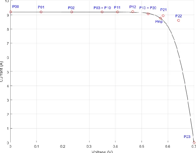
Figure 9 shows the location of the control points with respect to the I-V characteristic of the PV cell. The control points 𝑃00, 𝑃01, 𝑃02, 𝑃03= 𝑃10 and 𝑃11 are collinear and with 𝑃𝑚𝑝, are all being placed on the I-V characteristic.
Figure 9. PV cell I-V characteristic (black line, continuous) and the position of the 12 computed control points (red markers).
Figure 10. I-V characteristic of a PV cell modeled with three cubic Bézier curves, defined by 12 control points.
The relative error of the Bézier modeled I-V characteristic against the actual data taken from [12] is shown in Figure 11. It must be emphasized that in the 0 … 0.94 𝑉𝑜𝑐 range, the relative error is below 1%. Above 0.94 𝑉𝑜𝑐 the absolute error is less than 72mA, while the reference 𝐼𝑠𝑐= 9.207A.
Figure 11. The relative error of our model compared with the actual data. Good performance can be observed in the 0…0.5 V interval and near 𝑉𝑚𝑝. Higher errors occur near 𝑉𝑜𝑐 for low output currents.
4.3. Data fitting using the least squares method
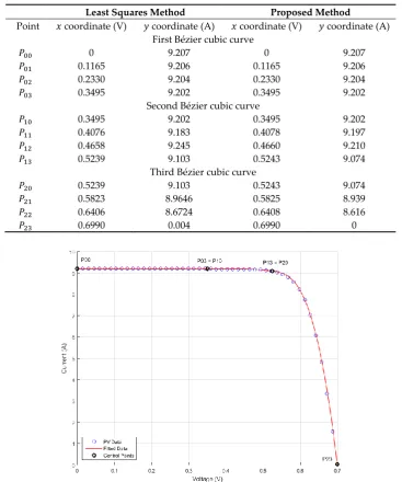
for Bézier curve fitting. In Section 4.2 we have shown that for the studied PV cell, the best results arise when the 𝑥 coordinates of the middle end points are set at 0.5𝑉𝑜𝑐 and 0.75𝑉𝑜𝑐 respectively. A similar conclusion arises if the least squares method is used for the same cell modeling. Running the least squares method for the MSMD290AS-36_EU Monocrystalline PV module proved that the minimum error occurs when the control end points are set again at 0.5𝑉𝑜𝑐 and 0.75𝑉𝑜𝑐 respectively. Table 5 summarizes the data fitting results for the same PV cell used in sections 4.1 and 4.2, where the results from the two approaches are very close. The graphical representation of the date fitting is given in Figure 12, where just the endpoints are represented.
Table 5. Control point coordinates comparison. On the left, the least squares method is used for computation, on the right the same values as in Table 4 are listed.
Least Squares Method Proposed Method
Point 𝑥 coordinate (V) 𝑦 coordinate (A) 𝑥 coordinate (V) 𝑦 coordinate (A) First Bézier cubic curve
𝑃00 0 9.207 0 9.207
𝑃01 0.1165 9.206 0.1165 9.206
𝑃02 0.2330 9.204 0.2330 9.204
𝑃03 0.3495 9.202 0.3495 9.202
Second Bézier cubic curve
𝑃10 0.3495 9.202 0.3495 9.202
𝑃11 0.4076 9.183 0.4078 9.197
𝑃12 0.4658 9.245 0.4660 9.210
𝑃13 0.5239 9.103 0.5243 9.074
Third Bézier cubic curve
𝑃20 0.5239 9.103 0.5243 9.074
𝑃21 0.5823 8.9646 0.5825 8.939
𝑃22 0.6406 8.6724 0.6408 8.616
𝑃23 0.6990 0.004 0.6990 0
Figure 12. Bézier approximation using the least squares method.
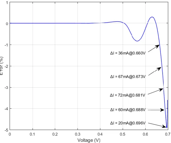
Figure 13. The relative error of the least squares method Bézier based approximation compared with the actual data. The absolute error ∆𝐼 = 𝐼𝐵𝑒𝑧𝑖𝑒𝑟− 𝐼 is also indicated.
4.4. Parameters variation
In order to further validate the proposed method, in this section we analyze the temperature and irradiance influence for the MSMD290AS-36_EU Monocrystalline PV module. An extensive study of the parameters influence over the PV cell can be found in [12]. It is important to notice that the Bézier approximation is not related to any of these parameters variation, just to the specified points 𝑃𝑠𝑐, 𝑃𝑚𝑝, 𝑃𝑜𝑐 and the parasitic resistances 𝑅𝑠ℎ0 and 𝑅𝑠0 as already stated. The challenge becomes in this case the finding of the new position for the control points and the new values for the parasitic resistances.
Villalva et al. [5] accurately describe the short circuit current variation as in (22):
𝐼𝑠𝑐 = (𝑅𝑠ℎ+ 𝑅𝑠
𝑅𝑠ℎ 𝐼𝑠𝑐,𝑟𝑒𝑓+ 𝑘𝐼∆𝑇) 𝐺
𝐺𝑟𝑒𝑓≈ (𝐼𝑠𝑐,𝑟𝑒𝑓+ 𝑘𝐼∆𝑇) 𝐺
𝐺𝑟𝑒𝑓 (22)
Ishaque and Salam [9] propose for the 𝑉𝑜𝑐,𝑐𝑒𝑙𝑙 the following variation (23):
𝑉𝑜𝑐,𝑐𝑒𝑙𝑙 = 𝑉0𝑐,𝑐𝑒𝑙𝑙,𝑟𝑒𝑓+ 𝑎 𝑘𝑇
𝑞 𝑙𝑛 𝐺 𝐺𝑟𝑒𝑓
+ 𝑘𝑣∆𝑇 (23)
Equation (23) proved to be too conservative in this case, as larger 𝑉𝑜𝑐,𝑐𝑒𝑙𝑙 variations were observed. A better approximation is the empirical law (24):
𝑉𝑜𝑐= 29.579 + 2.1934 ln 𝐺 (24)
A possible way for defining 𝑅𝑠ℎ behavior is suggested in [12], as in (25) with 𝑘𝑅𝑠ℎ estimated as 8 for the best fit.
𝑅𝑠ℎ= 𝑅𝑠ℎ,𝑟𝑒𝑓( 𝑇𝑟𝑒𝑓
𝑇 ) 𝑘𝑅𝑠ℎ
(25)
For 𝑅𝑠, a linear variation law (26) is given in [12] with 𝛼𝑅𝑠= −0.01K−1, again for the best fit:
Figure 14 shows the irradiance influence for the I-V module characteristic, where the approximated data using our proposed method is plotted with solid lines and the experimental data is represented with markers. 𝐼𝑠𝑐, 𝑉𝑜𝑐, 𝑅𝑠ℎ and 𝑅𝑠 were computed using (22), (24), (25) and (26) respectively.
Figure 14. Bézier approximation of the I-V irradiance dependent characteristics for the MSMD290AS-36_EU monocrystalline PV module. The lines represent the computed curves, whereas the markers represent the actual data.
The temperature dependent Bézier curves resulted from our algorithm compared with the actual data are introduced in Figure 15. Once again, the results show a very good correlation between the modeled data and the actual data.
4.5. Final validation
In order to definitely test whether the proposed method is applicable to common PV cells and modules, a selection of 18 cases have been analyzed at reference conditions, based on information found in their technical data [30-44], synthesized in Table 6. The selection includes 3 mono-crystalline PV arrays (1-3), 9 poly-crystalline arrays (4-11 and 13) and 1 poly-crystalline PV cell (12), a thin-film array (14), one Heterojunction with Intrinsic Thin layer (HIT, 15) 2 amorphous silicon glass arrays (with different see-through degrees, respectively 10% and 30%, 16 and 17) and eventually an amorphous Silicon cell (18).
Table 6. Datasheet technical data for the analyzed 18 PV cells and modules [30-44].
# PV Type Tech 𝒏𝒔 𝑽(𝑽) 𝒐𝒄 𝑽𝒎𝒑
(𝑽) 𝑰𝒎𝒑 (𝑨) 𝑰𝒔𝒄 (𝑨) 𝒌𝑽 (𝐕/𝐊) 𝒌𝑰 (𝐀/𝐊) 1 Shell SP-70 Mono 36 21.4 16.5 4.24 4.7 -0.076 0.002 2 Isofoton I150 InDach Mono 36 22.6 18.5 8.12 8.7 -0.1026 0.00365 3 Bosch M245 3BB Mono 60 37.8 30.11 8.14 8.72 -0.11718 0.002703 4 MSP300AS-36.EU Poly 72 44.48 37.42 8.02 8.58 -0.14678 0.003432 5 Kyocera KG200GT Poly 54 32.9 26.3 7.61 8.21 -0.123 0.00318 6 Kyocera KC85T Poly 36 21.7 17.4 5.02 5.34 -0.0821 0.00212 7 Kyocera KD135SX_UPU Poly 36 22.1 17.7 7.63 8.37 -0.08 0.00502 8 Kyocera KD245GH-4FB2 Poly 60 36.9 29.8 8.23 8.91 -0.133 0.00535 9 Sharp ND-224uC1 Poly 60 36.6 29.3 7.66 8.33 -0.13176 0.004415 10 Shell S36 Poly 36 21.4 16.5 2.18 2.3 -0.076 0.001 11 Solarex MSX-60 Poly 36 21.1 17.1
3.5 3.8 -0.08 0.003 12 Solarex MSX-60 - cell Poly 1 0.586 0.475 -0.00222
13 Amerisolar AS-6P 300W Poly 72 44.7 36.7 8.19 8.68 -0.14751 4.86E-03 14 Shell ST40 Thin-Film 36 23.3 16.6 2.41 2.68 -0.1 0.00035 15 Sanyo HIT-240 HDE4 HIT 60 43.6 35.5 6.77 7.37 -0.109 0.00221 16 Onyx 1200x600 Ref10
aSi glass 72 47 32 0.9 1.11 -0.0893 0.000999
17 Onyx 1200x600 Ref30 0.63 0.74 0.000666
18 6.5Wp L Cel aSi cell 1 2.2 1.6 4.09 5.1 -0.00836 0.00612
Using the Villalva algorithm [5], the main parameters were computed and listed in Table 7. For the last 3 cases, due to different technology, interesting values for the diode ideality factor 𝑎 occur.
Table 7. Computed values for main parameters of the analyzed PV cells and modules.
Table 8 lists the control points computed for Bézier curve fitting, where in all cases the control end points are set at 0.5𝑉𝑜𝑐 and 0.75𝑉𝑜𝑐 respectively. Just two 𝑥 coordinates are presented, as the others are evenly
spaced and can be easily computed. Selected plots of the PV devices are presented in Figure 16.
Table 8. Control points coordinates of the analyzed PV cells and modules.
x coord. (V) y coordinates (A)
# 03 13 00 01 02 03 11 12 13 21 22
1 10.628 15.931 4.732 4.684 4.637 4.588 4.538 4.606 4.360 4.212 2.575 2 11.295 16.930 8.703 8.690 8.678 8.663 8.635 8.696 8.508 8.210 8.125 3 18.870 28.285 8.735 8.706 8.678 8.649 8.604 8.697 8.453 8.529 5.997 4 22.224 33.312 8.586 8.547 8.509 8.470 8.443 8.453 8.370 7.684 9.991 5 16.425 24.620 8.223 8.194 8.167 8.137 8.094 8.178 7.930 7.909 5.930 6 10.845 16.256 5.343 5.335 5.327 5.318 5.298 5.350 5.212 5.200 4.168 7 10.975 16.451 8.401 8.3301 8.260 8.189 8.128 8.178 7.946 7.918 6.273 8 18.415 27.603 8.928 8.883 8.841 8.796 8.749 8.812 8.595 8.581 7.029 9 18.228 27.362 8.354 8.298 8.243 8.187 8.133 8.191 7.967 7.954 6.288 10 10.940 16.399 2.300 2.300 2.300 2.299 2.287 2.331 2.226 2.180 1.367 11 10.527 15.779 3.808 3.784 3.760 3.736 3.715 3.733 3.649 3.599 3.241 12 0.293 0.438 3.809 3.786 3.763 3.739 3.718 3.738 3.652 3.608 3.204 13 22.336 33.479 8.686 8.667 8.649 8.630 8.606 8.650 8.525 8.411 8.209 14 11.565 17.335 2.700 2.680 2.666 2.642 2.606 2.669 2.275 1.868 0.969 15 21.720 32.557 7.397 7.336 7.274 7.213 7.168 7.185 7.063 7.200 5.950 16 23.500 35.225 1.110 1.0717 1.0343 0.995 0.971 0.978 0.775 0.578 0.289 17 23.500 35.225 0.740 0.723 0.707 0.689 0.677 0.686 0.542 0.403 0.201 18 1.100 1.649 5.100 4.928 4.760 4.584 4.456 4.506 3.949 3.372 1.786
In the second column of Table 9, the average of the current (𝐼) relative error is displayed in order to evaluate the fit quality. Maximum current error (absolute and relative values) is listed in each case with the coordinates where it appears. The maximum power point is also investigated as an absolute and relative error and finally the computed value is listed. The current (𝐼) relative error is below 1.18% in all cases, and the 𝑃𝑚𝑝 relative error is even better (lower than 1% in all cases).
Table 9. Computed errors for the analyzed PV cells and modules.
Current (𝑰) Error Max. Power (𝑷𝒎𝒑) Error
# Avg.Rel. (%) Coordinates Abs. (mA) Rel. (%) Abs. (W) Rel. (%) Comp. (W) 𝑉 (V) 𝐼 (A)
(a) #3 Bosch M245 3BB
(b) #7 Kyocera KD135SX_UPU
(c) #10 Shell S36
(d) #12 MSX-60 Single Cell
(e) #16 Onyx Ref 10
(f) #18 6.5Wp L Cell
5. Discussion
In all studied cases, the 𝑥 coordinates can be evenly spaced. Both for the PV cells and for the PV modules, the first Bézier cubic curve was very close to a straight line and ended at 𝑥03= 0.5𝑉𝑜𝑐, while the middle curve ended at 𝑥13= 0.75𝑉𝑜𝑐. The relative error is less than or equal to 1.18% for all the studied PV devices.
The differences between the results obtained with the proposed method and the least squares method are negligible (less than 1% for all coordinates). 𝑅𝑠 and 𝑅𝑠ℎ can be easily derived from the manufacturer’s datasheet, using for example the method proposed by Vilallva et al. [5]. In most cases 𝑅𝑠ℎ is close to 𝑅𝑠ℎ𝑜 (Table 7). Larger differences occur for the series parasitic resistance: for the same PV cell. For different irradiances and temperatures, the section 4.4 provides all the necessary formulae.
In most cases 𝑉𝑚𝑝 > 𝑃13𝑥. The method was also valid for Onyx Ref 10, Onyx Ref 30 and 6.5Wp L Cell, where the previous relation was not satisfied.
In relation with the Maximum Power Point Tracking (MPPT), it must be emphasized that the Bézier curves are inherently smooth. This reduces the risk for the algorithm to get stuck in some false area/minimum of the curve. Furthermore, the generation of the Bézier curves being so easy, MPPT simulation can be further simplified.
6. Conclusions
A novel method for modeling a PV cell or a PV module I-V characteristic has been introduced. To the best of our knowledge, Bézier curves were not used to model the I-V characteristic of PV devices before. The method proved good accuracy and was validated both in the case of a single PV cell and in the case of a whole PV module, for different technologies and manufacturers. The method was also used in the case of varying irradiance and temperature. The proposed method can be used for implementing hardware solar array simulators, for teaching or remote study. It is far more easy to use the proposed method to find the I-V characteristic of a PV cell or module when compared with solving the exponential equations associated with the single or double diode model largely used today. A common microcontroller can compute the points on the I-V curve with a minimum of resources, inherently increasing the computing speed and the response of the system.
The advantage of our method relies in the ease of I-V characteristic generation: if we exclude 𝑉𝑜𝑐 and 𝐼𝑠𝑐, only 10 different values (𝑃23𝑥= 𝑉𝑜𝑐, 𝑃00𝑦= 𝐼𝑠𝑐, 𝑃01𝑦, 𝑃02𝑦, 𝑃03𝑦, 𝑃11𝑦 , 𝑃12𝑦, 𝑃13𝑦, 𝑃21𝑦, 𝑃22𝑦) have to be stored – SAS manufacturers usually use 1024 or more double points to accurately define the I-V characteristic. Alternate use is for any graphical plot of the I-V (and subsequently P-V) curves. Furthermore, little knowledge of the device itself is required, as only common data from the datasheet is needed.
Acknowledgments: This work was supported by both the Romanian National Authority for Scientific Research and Innovation, CNCS/CCCDI-UEFISCDI within PNCDI III, project number PN-III-P2-2.1-PED-2016-0074 and by Politehnica University Timisoara, according to the Administration Board research policy.
Author Contributions: Both authors have contributed to this research. Aurel Gontean conceived and designed the study and carried out the simulations. Roland Szabo analyzed the data. Aurel Gontean wrote the paper and reviewed the manuscript. Both authors read and approved the manuscript.
Conflicts of Interest: The authors declare no conflict of interest.
Nomenclature
Main Symbols
𝑎 Diode ideality factor 𝐺 Actual irradiance
𝐺𝑟𝑒𝑓 Reference irradiance, 1000 W/m2
𝐼 Output current
𝐼𝑠𝑐 Short circuit current
𝐼𝑠𝑐,𝑟𝑒𝑓 Short circuit current 25°C
𝑘 Boltzmann constant
𝑘𝐼 Current temperature coefficient, A/K
𝑘𝑉 Voltage temperature coefficient, V/K
𝑘𝑅𝑠ℎ 𝑅𝑠ℎtemperature exponent
𝑛𝑠 Number of series cells
𝑃𝑚𝑝= 𝑉𝑚𝑝𝐼𝑚𝑝 Maximum output power
𝑞 Electron charge 𝑅𝑠 Series resistance
𝑅𝑠,𝑟𝑒𝑓 Series resistance at 25°C
𝑅𝑠0 Series resistance based on I-V characteristic slope close to 𝑉𝑜𝑐
𝑅𝑠ℎ Parallel (shunt) resistance
𝑅𝑠ℎ,𝑟𝑒𝑓 Parallel (shunt) resistance, at 25°C
𝑅𝑠ℎ0 Parallel (shunt) resistance based on I-V characteristic slope close to 𝐼𝑠𝑐
𝑇 Internal temperature, [K] 𝑇𝑟𝑒𝑓 Reference temperature 298.15 K
∆𝑇 = 𝑇 − 𝑇𝑟𝑒𝑓 Temperature difference
𝑉 Output voltage 𝑉𝑜𝑐 Open circuit voltage
𝑉𝑜𝑐,𝑟𝑒𝑓 Open circuit reference voltage at 25°C
𝑉𝑜𝑐,𝑐𝑒𝑙𝑙 Solar cell open circuit voltage
𝑉𝑜𝑐,𝑐𝑒𝑙𝑙,𝑟𝑒𝑓 Solar cell open circuit reference voltage at 25°C
𝑉𝑚𝑝 Output voltage at maximum power point
Abbreviations
AM Air Mass
MPPT Maximum Power Point Tracking
PV Photovoltaic
SAS Solar Array Simulator
STC Standard Test Conditions (cell temp. 25°C; irradiance 1000 W/m2; air mass 1.5)
Greek Symbols
𝛼𝑅𝑠 Series resistance temperature coefficient (linear law)
References
1. 4Q 2017 Frontier Power Market Outlook, https://about.bnef.com/blog/4q-2017-frontier-power-market-outlook/ (accessed on 3 January 2018).
2. Solar PV 2018, https://www.pv-magazine.com/2017/12/01/solar-pv-2018-installs-of-111-gw-a-polysilicon-factory-boom-and-0-30w-for-modules-2/ (accessed on 3 January 2018).
3. Phang, J.C.H.; Chan, D.S.H.; Phillips, J.R. Accurate Analytical Method For The Extraction Of Solar Cell Model Parameters, Electron Lett1984, 20(10), pp. 406 – 408, DOI: 10.1049/el:19840281.
4. Garrido-Alzar, C.L. Algorithm for extraction of solar cell parameters from I-V curve using double exponential mode, Renew Energy 1997, 10 (2-3), pp. 125-128, https://doi.org/10.1016/0960-1481(96)00049-3. 5. Villalva, M.G.; Gazoli, J.R.; Filho, E.R. Comprehensive Approach to Modeling and Simulation of
Photovoltaic Arrays, IEEE Trans. Power Electr.2009, 24, pp. 1198–1208.
6. Babu, B.C.; Gurjar, S. A novel simplified two-diode model of photovoltaic (PV) module, IEEE J Photovolt 2014, 4(4), 2014, pp. 1156-1161, DOI: 10.1109/JPHOTOV.2014.2316371.
7. Cubas, J.; Pindado, S.; de Manuel, C. Explicit Expressions for Solar Panel Equivalent Circuit Parameters Based on Analytical Formulation and the Lambert W-Function, Energies2014, 7, pp. 4098–4115.
9. Ishaque, K.; Salam, Z. An improved modeling method to determine the model parameters of photovoltaic (PV) modules using differential evolution (DE), Sol Energy 2011, 85(9), pp. 2349 – 2359, DOI: 10.1016/j.solener.2011.06.025.
10. Franzitta, V.; Orioli, A.; Di Gangi, A. Assessment of the Usability and Accuracy of the Simplified One-Diode Models for Photovoltaic Modules, Energies2016, 9, 1019, DOI:10.3390/en9121019.
11. Franzitta, V.; Orioli, A.; Gangi, A.D. Assessment of the Usability and Accuracy of Two-Diode Models for Photovoltaic Modules, Energies2017, 10, 564, DOI:10.3390/en10040564.
12. Gontean, A.; Lica, S.; Bularka, S.; Szabo, R.; Lascu, D. A Novel High Accuracy PV Cell Model Including Self Heating and Parameter Variation, Energies2018, 11, 36, doi:10.3390/en11010036.
13. Cuce, E.; Cuce P.M.; Karakas I.H.; Bali, T. An accurate model for photovoltaic (PV) modules to determine electrical characteristics and thermodynamic performance parameters, Energ Convers Manage2017 146, pp. 205–216, https://doi.org/10.1016/j.enconman.2017.05.022.
14. Farin, G. A History of Curves and Surfaces in CAGD, in Handbook of Computer Aided Geometric Design; Farin, G.E.; Hoschek, J., Kim, M.S. Eds.; Elsevier, Amsterdam, The Netherlands, 2002; pp. 1–22, ISBN 978-0-444-51104-1, https://doi.org/10.1016/B978-0-444-51104-1.50035-6.
15. Farin, G. Curves and Surfaces for CAGD. A Practical Guide, 5th Edition, Academic Press, San Francisco, CA, USA, 2002, pp. 81 – 95, ISBN: 1-55860-737-4, https://doi.org/10.1016/B978-1-55860-737-8.50032-6.
16. Mortenson, M.E. Geometric modeling, 3rd Edition, Industrial Press, South Norwalk CT, USA 2006, ISBN 978-0-831-13298-9.
17. Farin, G. Shape Representation, in Wiley Encyclopedia of Electrical and Electronics Engineering, Published Online: 13 Jul 2007, http://onlinelibrary.wiley.com/doi/10.1002/047134608X.W7525.pub2/full, ISBN: 978-0-471-34608-1, DOI: 10.1002/047134608X.
18. Tromba, D.; Munteanu, L.; Schneider, V.; Holzapfel, F. Approach trajectory generation using Bézier curves, 2015 IEEE International Conference on Aerospace Electronics and Remote Sensing Technology (ICARES), 3-5 Dec. 2015, DOI: 10.1109/ICARES.2015.7429835
19. Jalba, A.C.; Wilkinson, M.; Roerdink J. Shape representation and recognition through morphological curvature scale spaces, IEEE Trans Image Process, 2006 15 (2), pp. 331 - 341, DOI: 10.1109/TIP.2005.860606. 20. Prautzsch, H.; Boehm, W.; Paluszny M. Bézier and B-Spline Techniques, Spinger, Berlin, Germany, 2002, pp.
9 – 57, ISBN 3-540-43761-4.
21. 156 mm Monocrystalline Mono Solar Cell 6 x 6. Available online: https://www.aliexpress.com/item/50pcs-lot-4-6W-156mm-mono-solar-cells-6x6-150feet-Tabbing-Wire-15feet-Busbar-Wire-1pc/1932804007.html (accessed on 21 Sep 2017).
22. MünchenSolar M Series Monocrystalline MSMDxxxAS-36.EU Datasheet, https://cdn.enf.com.cn/Product/pdf/Crystalline/559cd7e85436f.pdf (accessed on 31 Jan 2018)
23. Mugnaini, D. Bézier Curve with draggable control points. Draw, manipulate and reconstruct Bézier Curves, version 1.11, Available online: https://www.mathworks.com/matlabcentral/fileexchange/51046-bézier-curve-with-draggable-control-points (accessed on 30 Dec 2017)
24. Garrity, M. Bézier Curves and Kronecker's Tensor Product, posted 13 October 2014, Available online: https://blogs.mathworks.com/graphics/2014/10/13/bézier-curves/, (accessed on 31 Dec 2017)
25. Khan, M. Cubic Bézier Least Square Fitting, version 1.4, https://www.mathworks.com/matlabcentral/fileexchange/15542-cubic-bézier-least-square-fitting,
(accessed on 30 December 2017).
26. Wolberg, J. Data Analysis Using the Method of Least Squares. Extracting the Most Information from Experiments, 2006 Springer-Verlag Berlin Heidelberg, ISBN 978-3-540-25674-8, DOI 10.1007/3-540-31720-1
27. Hansen pC.; Pereyra V.; Scherer G. Least Squares Data Fitting with Applications, JHU Press, Baltimore, USA, 2013, ISBN 978-1-421-40786-9.
28. Shao, L.; Zhou, H. Curve Fitting with Bézier Cubics, in Graphical Models and Image Processing, Volume 58, Issue 3, May 1996, Pages 223-232, https://doi.org/10.1006/gmip.1996.0019.
29. Zhao, L.; Jiang, J.; Song, C.; Bao, L.; Gao, J., Parameter Optimization for Bézier Curve Fitting Based on Genetic Algorithm, in: Tan Y., Shi Y., Mo H. (eds) Advances in Swarm Intelligence, ICSI 2013, Lecture Notes in Computer Science, vol 7928. Springer, Berlin, DOI: https://doi.org/10.1007/978-3-642-38703-6_53. 30. Shell SP70 Photovoltaic Solar Module, Product Information Sheet,
31. Isofoton I-150 InDach Solar Panel specifications, http://www.posharp.com/i-150-indach-solar-panel-from-isofoton_p337595585d.aspx (accessed on 15 Mar 2018)
32. Bosch Solar Module c-Si M 60 Model M245 3BB, http://www.bosch-solarenergy.de/media/us/alle_pdfs_1/technische_dokumente_3/datenblaetter_1/kristalline_module_6/p_6 0_eu30014_1/Bosch_Solar_Module_c_Si_M_60_EU30014_en_Europe.pdf (accessed on 16 Mar 2018)
33. München Solarenergie GmbH MSP300AS-36.EU,
http://www.secondsol.de/handelsplatz/herstellerdatenblatt/photovoltaikmodule/Polykristallin/M%C3%B Cnchen%20Solarenergie%20GmbH/MSP300AS-36.EU.htm (accessed on 16 Mar 2018)
34. Kyocera KC200GT, High Efficiency Multicrystal Photovoltaic Module, https://www.kyocerasolar.com/dealers/product-center/archives/spec-sheets/KC200GT.pdf (accessed on 16 Mar 2018)
35. Kyocera KC85T, High Efficiency Multicrystal Photovoltaic Module, https://www.kyocerasolar.com/dealers/product-center/archives/spec-sheets/KC85T.pdf (accessed on 17 Mar 2018)
36. Kyocera KD245GH-4FB2 High Efficiency Multi-Crystalline Photovoltaic Module, http://www.australiansolar.com.au/images/KD245GH-4FB2.pdf (accessed on 17 Mar 2018)
37. Kyocera KD135SX_UPU Technical Data,
http://www.datasheetspdf.com/pdf/846173/KYOCERA/KD135SX-UPU/1 (accessed on 17 Mar 2018) 38. Sharp ND-224UC1 (224W) Solar Panel Technical Data,
http://files.sharpusa.com/Downloads/Solar/Products/sol_dow_ND224UC1.pdf (accessed on 17 Mar 2018) 39. Shell Solar Revised 2nd Ed.
http://www.efn-uk.org/l-street/renewables-lib/solar-reports/index_files/Shell-Solar.pdf (accessed on 18 Mar 2018)
40. Solarex MSX-60 and MSX-64 Photovoltaic Modules Technical Data, https://www.solarelectricsupply.com/media/custom/upload/Solarex-MSX64.pdf (accessed on 18 Mar 2018)
41. Amerisolar AS-6P Technical Data,
https://www.acosolar.com/amfilerating/file/download/file_id/448/?___store=solar_all (accessed on 18 Mar 2018)
42. Sanyo HIT-240 HDE4 Technical Data, http://future-energy-solutions.co.uk/wp-content/uploads/2014/10/Panasonic-Datasheet-HIT-240W.pdf (accessed on 18 Mar 2018)
43. Onyx 1200x600 ref10 Technical Data, http://onyxsolardownloads.com/docs/ALL-YOU-NEED/Technical_Guide.pdf (accessed on 17 Mar 2018)