systems
Florimond Guéniat, Lionel Mathelin, and Luc R. Pastur
Citation: Physics of Fluids (1994-present) 27, 025113 (2015); doi: 10.1063/1.4908073 View online: http://dx.doi.org/10.1063/1.4908073
View Table of Contents: http://scitation.aip.org/content/aip/journal/pof2/27/2?ver=pdfcov Published by the AIP Publishing
Articles you may be interested in
Molecular dynamics investigation of nanoscale cavitation dynamics J. Chem. Phys. 141, 234508 (2014); 10.1063/1.4903783
A Lagrangian subgrid-scale model with dynamic estimation of Lagrangian time scale for large eddy simulation of complex flows
Phys. Fluids 24, 085101 (2012); 10.1063/1.4737656
The effects of non-normality and nonlinearity of the Navier–Stokes operator on the dynamics of a large laminar separation bubble
Phys. Fluids 22, 014102 (2010); 10.1063/1.3276903
A dynamic global-coefficient subgrid-scale model for large-eddy simulation of turbulent scalar transport in complex geometries
Phys. Fluids 21, 045109 (2009); 10.1063/1.3115068
A dynamic mode decomposition approach for large
and arbitrarily sampled systems
Florimond Guéniat,1,2Lionel Mathelin,1and Luc R. Pastur1,2
1LIMSI-CNRS, 91403 Orsay Cedex, France 2Paris Sud University, 91400 Orsay Cedex, France
(Received 6 June 2014; accepted 2 February 2015; published online 19 February 2015)
Detection of coherent structures is of crucial importance for understanding the dynamics of a fluid flow. In this regard, the recently introduced Dynamic Mode Decomposition (DMD) has raised an increasing interest in the community. It allows to efficiently determine the dominant spatial modes, and their associated growth rate and frequency in time, responsible for describing the time-evolution of an observation of the physical system at hand. However, the underlying algorithm requires uniformly sampled and time-resolved data, which may limit its usability in practical situations. Further, the computational cost associated with the DMD analysis of a large dataset is high, both in terms of central processing unit and memory. In this contribution, we present an alternative algorithm to achieve this decomposition, overcoming the above-mentioned limitations. A synthetic case, a two-dimensional restriction of an experimental flow over an open cavity, and a large-scale three-dimensional simulation, provide examples to illustrate the method. C 2015 AIP Publishing LLC.
[http://dx.doi.org/10.1063/1.4908073]
I. INTRODUCTION
Identification of coherent structures is nowadays a pivotal instrument for understanding the phenomenology and dynamics of a fluid flow. A powerful analysis tool, the dynamic mode decom-position (DMD), has recently been introduced.19,20 Dynamic modes reveal spatial coherent
struc-tures associated with temporal spectral components, including temporal growth rates. It has been shown in Ref.3 that Dynamic Mode Decomposition is connected to discrete Fourier transform, while14discussed the connection between DMD and Koopman analysis, inherited from the dynam-ical system theory. Dynamic modes are therefore informative of the dynamdynam-ical skeleton of a flow. DMD has been successfully applied to a wide range of systems, in particular, fluid flows such as cavity flows,9,20,22or jet flows,21,23among others. Some recent developments include error analysis of the identified growth rates,7and improvements on the approximation method.3,11
Dynamic Mode Decomposition requires time-resolved data, uniformly sampled in time. The time interval must be chosen small enough so as to resolve all time-scales of interest of the under-lying dynamics. This sampling strategy brings severe constraints on the measurement workflow. As an example, consider the typical situation where the observable (sample) is a two-dimensional (2-D), two-component (2-C), velocity field acquired with a Particle Imagery Velocimetry (PIV) technique. Standard in PIV are fields of 1000×1000 pixels. Suppose the highest frequency of interest in the flow field is 200 Hz, a mild assumption, the Shannon-Nyquist criterion imposes a sampling frequency above 400 Hz to resolve the fast time scales of the flow. With 12-bit images, the resulting data rate is then already above 1 GB/s. Further, if the Fourier spectrum is wide-banded, the timespan of the acquisition procedure has to be large to capture the low frequency components. The combination of a high sampling frequency and a long acquisition sequence then quickly results in intractable constraints, both on the measurement chain hardware and the computational resources. This, of course, also applies when considering time-resolved datasets from numerical computations. Another limitation is that observation data could be corrupted from external or intrinsic sources, say from the experimental setup. As a typical example, one can think of acquisition failure or
1070-6631/2015/27(2)/025113/17/$30.00 27, 025113-1 ©2015 AIP Publishing LLC
corrupted images in PIV. Physically irrelevant information is then introduced when correcting such perturbations and adversely affects the standard DMD accuracy.
In this paper, we address these above-mentioned limitations. The method we present can essen-tially rely on asubsetof the observation data, both in the spatial and time domains, hence naturally handling corrupted or missing data and arbitrary sampling. The resulting small and scattered dataset is suitably handled by techniques focusing the scarce available information on the dominant approx-imation modes by exploiting the compressibility of the decomposition in the retained format. The selection of the subset could rely on Fourier spectra estimated with a compressed sensing technique, see Ref.5, among many others for an introduction to the theory. To avoid the computational cost associated with the compressed sensing problem, a suboptimal criterion based on statistics of the time-series is employed. Thanks to working on a subset of the original data, the computational burden is, sometimes drastically, alleviated compared to the standard DMD method, consequently allowing very large flow fields, and/or systems with a wide spectrum, to be analyzed. The key of the proposed method is to decouple the identification of the dominant temporal scales from their associated spatial modes.
Preliminary results of the present contribution were introduced in Ref.10. A recent effort,11 discusses the use of compressed sensing to select dominant DMD modes. Our method is different in the sense that it is not ana posterioriapproach relying on a standard DMD, and hence subjected to its limitations, but instead directly determines the dominant dynamic modes from an (almost) arbitrary dataset.
After the standard DMD algorithm is briefly recalled in Sec. II, the different aspects of the proposed method are introduced in Sec. III. They are illustrated and compared with a standard DMD analysis on a synthetic 2-D dataset and a 2-D space- and time-resolved experimental dataset from the flow over an open cavity in Sec.IV. A three-dimensional numerical simulation, involving more than 2×10⁶spatial degrees-of-freedom, is also considered to illustrate the applicability of the
present approach to large-scale situations. Closing remarks conclude the paper in Sec.V.
II. DYNAMICAL MODE DECOMPOSITION
In this section, we briefly recall the dynamic mode decomposition algorithm. More details can be found in Refs.19and20.
We are interested in characterizing the linear, time-invariant, operatorAmapping a real-valued observation vectorun∈Rnpof the physical system at hand at timetnto the observationun+1when
a time∆thas elapsed,tn+1=tn+∆t. Rearranging a sequenceKB(u1. . .uN)∈Rnp×NofN
snap-shots in matricesK1B(u1. . .uN−1)andK2B(u2. . .uN)∈Rnp×(N−1)results in characterizing the
properties ofAsuch that
AK1=K2. (1)
Introducing the economy-size singular value decomposition (SVD) of K1≡UΣW∗, withW∗ the
Hermitian transpose ofW, Eq. (1) leads to
AUBUU∗AU=U U∗K2WΣ−1
CS
. (2)
The matrixSBU∗K2WΣ−1is similar to A, the approximation of Ain the column space ofK1, so that its eigenvalues{λk}k are eigenvalues of A, and eigenvectors{ϕk}k of S are related to
eigen-vectors{φk}k (i.e., dynamic modes) of Aviaφk ≡Uϕk,∀k. Sinceλs are complex, they express
as
λk=ρkexp
(√
−1ωk∆t
)
, ∀k. (3)
Any eigenvalue is hence related to a frequency fk=ωk/2π and each spatial mode φk is,
III. IDENTIFICATION OF DYNAMIC MODES FROM ARBITRARY DATA
A. Efficient use of the available data
As discussed in the Introduction, the standard dynamic mode decomposition approach pre-sented above is restricted to data available in a strict format since the sampling must be uniform in time (so that the snapshots matrix K can be associated with a Krylov matrix) and the entire spatial field is considered. In many situations, the resulting decomposition exhibits some dynamic modes which are dominant with respect to some others and one is typically interested in char-acterizing these dominant modes only—in a nutshell, the real part ℜ[φk] of a spatial mode φk
considered as dominant lies in a cone of small mean angle∠kBN−1Nn ∠k,nfrom the snapshots,
with∠k,n∈[−π, π], cos(∠k,n)=ℜ[φk]∗un ∥un∥2−1 ∥ℜ[φk]∥
−1
2 . When the spectrum of the
decom-position is sparse, in the sense that only a limited number of modes is responsible for describing most of the dynamics, the number of dominant modes is small and they hence require only a small amount of information to be determined. It results that the standard Krylov matrix K contains significantly more information than actually needed for this objective. This also suggests a route for a tractable DMD when the dataset is very large and cannot be processed by a standard DMD.
The key of the method we now expose is to extract information relevant for the dominant modes from scarce data (small dataset). To this end, the determination of the spectral features of the dominant modes is decoupled from the approximation of their spatial description, in contrast with the standard DMD where the two aspects are intricately coupled in the eigenproblem issued from Eq. (2).
To proceed, we rely on an alternative description of the dataset in a similar spirit as in Ref.3. The DMD analysis leads to a decomposition of the observable on a spatial basis with complex temporal coefficients,
u(tn)Cun≈ Nmd
k=1
ρn ke
√
−1ωkn∆tφ k≡
Nmd
k=1
λnkφk, (4)
withNmdis the number of modes retained for the approximation andtngiven astn=n∆t,n∈N.
The dataset K can then be approximated in terms of spatial modes {φk} Nmd k=1 ∈C
np and temporal coefficients{λk}
Nmd
k=1 ∈C. From Eq. (4), the set of snapshotsKmay be expressed as
K =MΛ+Res, (5)
whereRes∈Cnp×Nis a residual,M ∈Cnp×Nmdcontains theNmddominant spatial modes,
M B φ1. . .φNmd
,
(6)
andΛ∈CNmd×N is a pseudo-Vandermonde matrix containing the associated N
mdtemporal coeffi
-cients, ΛB * . . . . . . . ,
λ11 λ21 · · · λ1N λ12 λ22 · · · λ2N
..
. ... . .. ...
λ1N
md λ
2
Nmd · · · λ N Nmd + / / / / / / / -. (7)
B. Non-uniform sampling
One can relax the constraint on the uniform sampling in time and account for snapshots sampled at arbitrary times. When dealing with a non-uniform sampling, the standard DMD algo-rithm fails since Eq. (1) does then not hold. However, for an arbitrary timetn∈R, the
approxima-tion (4) writes
utn≈λ
tn 1 φ1+λ
tn
2 φ2+. . .+λ
tn
NmdφNmd, ∀tn∈R, (8)
and the, now alternant, matrixΛnow reads Λ= * . . . . . . . , λt1
1 λ
t2
1 · · · λ
tN 1 λt1
2 λ
t2
2 · · · λ
tN 2
..
. ... . .. ...
λt1
Nmd λ
t2
Nmd · · · λ
tN Nmd + / / / / / / / -, (9)
where{t1,t2, . . . ,tN}∈RNis arbitrary. Without loss of generality, we set the time reference tot1so
thattref← t1,tn← tn−tref,1≤n≤N.
The approximation of the dynamics of the system can then be derived from matricesΛandM. Provided the norm, in the Frobenius sense, of the residualResis small,Mcan be well approximated from Eq. (5) by
M ≈KΛ+. (10)
Substituting M from (10) in (5) leads to K≈KΛ+Λ+Res, with Λ+ the Moore-Penrose pseudo-inverse ofΛ.Λis then determined by minimizing the Frobenius norm of the residualRes,
Res≈K IN−Λ+Λ
,
(11)
and spatial modes{φk} Nmd k=1 ∈C
npfollow immediately from Eq. (10).
The temporal information of theNmddominant modes is entirely given byλB λ1. . .λNmd
∈
CNmd and then requires no more than 2 Nmd pieces of information to be estimated. A very low
numberNof snapshots is then sufficient in principle.
Since a low number of modes is supposed dominant, the temporal spectrum of the system at hand is sparse in a Fourier basis (few dominant frequencies) and can then be well approxi-mated from a limited number of snapshots via a residual norm minimization under a cardinality constraint as justified by the compressed sensing theory for the linear situation.1,2,5 In particular, the Shannon-Nyquist sampling limitations do not apply in this context and an observable with a wide-banded, but sparse or even just compressible, spectrum can be effectively retrieved via this technique as the provided examples will demonstrate in Sec.IV. Instead of a penalty on the effective cardinality of the set of dominant DMD modes, we here directly choose the number of approximation modesNmd. It results in an optimization problem such as
λ∈arg min
λ∈CNmd
K (
IN−Λ
( λ )+ Λ(λ )) F , (12)
with entries ofΛcomputed fromλ, cf. Eq. (9). The modes are then given byM=KΛ+. Notice that, sinceΛ∈CNmd×N, the matrixΛ+Λis a square, rank-N
md, matrix of size N×N. Since Nmd≪N, Λ+Λ is highly rank-deficient and cannot get close to IN in the sense of ∥·∥F for any λ. Upon
evaluation of the economy-size QR decomposition of the snapshot matrix,Q RQR= K,Q∈Rnp×N
andR∈RN×N, and since left-multiplication of a matrix by a unit-normed column matrix does not
change its Frobenius norm, the optimization problem (12) finally reduces to
λ∈arg min
λ∈CNmd
R (
IN−Λ
( λ )+ Λ(λ )) F , (13)
which only involves matrices of the size of the number of snapshotsN, rather than the sizenpof the
snapshots themselves.
This approach allows to rely on scarce data, requiring only a low number of snapshotsN and hence resulting in tractable matricesR, IN, andΛ. SinceNmdis low, the optimization problem is
low-dimensional and can be efficiently solved, either inR2Nmdwith algorithms possibly as simple
as the derivative-free Nelder-Mead method,12 used in the present work or directly in
CNmd, see
C. Large dataset
1. General comments
Similarly to datasets with a large number of snapshots, performing a standard DMD analysis on a dataset with large snapshot vectors such as those from, say, 3-D flow fields, is computation-ally challenging. In the typical case where np≫N, the overall computational cost of the SVD,
as required by the standard DMD algorithm, is O npN2
, which may be prohibitive in case of 3-D space and time-resolved datasets from direct numerical simulations. Similarly, the amount of memory needed for the SVD may limit the use of standard DMD.
Further, while the QR decomposition of the Krylov matrix K makes optimization problem (13) independent of the size of the snapshots, and hence potentially suitable for large fields, an
np×N-matrix still needs be stored in memory to achieve the QR decomposition, even using
incremental algorithms.
The Takens’ theorem28suggests that the time series of a well observable quantity may contain
the full dynamics of the underlying dynamical system. Since the spatial support associated with a given time evolution pattern is often large, as shown by Robinson,17a space-decimated observable vector may then be a relevant approximation to capture the temporal features of the flow. As already discussed in Secs. III A andIII B, the dominant features of the flow are often described by a few degrees of freedom and scarce data may suffice to accurately approximate them. This idea is further supported by the fact that the Koopman operator—which has been shown to be related to the DMD in the sense that the DMD algorithm results in the estimation of the eigenvalues of the Koopman operator associated with the dynamics14,19—is defined only by the dynamical flow and should therefore be independent from the choice of the observable. Changing the observable does then not change the eigenvalues of the evolution operatorA.
We now further improve upon the NU-DMD algorithm introduced in Sec. III B. Our strat-egy is to decimate the original datasetK by selecting a low numbernp of components,np<np. Consequently, space-decimated observablesun∈R
npare constructed, and a new, smaller, dataset
K
np∈R
np×N follows. A DMD, or NU-DMD, analysis is then carried-out on the resulting small
dataset. The NU-DMD optimization problem (Eq. (13)) now formulates as31
λ ∈arg min
λ∈CNmd
K
np IN−Λ+Λ
F
, (14)
M=KΛ+. (15)
Since the optimization problem (14) involves small matrices (both N andnp are small), this algorithm allows the computation of a few dominant modes with low computational requirements.
2. Subset selection
The selection of the spatial components of K retained in the space-decimatedK
np must be such that their cardinalitynpis low, allowing for a computationally efficient optimization problem
(14), while retaining relevant temporal information so that the frequency and growth rates of the dominant modes can be accurately estimated. The subset selection problem can then formulate as finding the set of indicesJ =j1,j2, . . . ,jnp
, 1≤ ji∈N≤np, so thatλderived fromK
npvia (14) is a good approximation ofλderived from K via (12). The idea is to cluster spatial components whose dynamics are similar. One must then determine the dominant Fourier spectrum of the discrete time series of components of the observable,
u(i)(t)=(u(i)(t1)u(i)(t2). . .u(i)(tN)
)T
∈RN, (16)
with 1≤i ≤np. In case the sampling is non-uniform in time, as considered in Sec. III B, a
discrete Fourier transform cannot be applied. One then resorts to a minimization problem to determine the Nf dominant Fourier modes that best approximate the time-series in the form
u(i)(t)≈Na
k a
(i)
k exp
(√
−1ωkt
)
,∀1≤i ≤np,
a(i)∈ arg min a (i)∈ CNa
u(i)(t)− ℜΨa(i)
2
,
s.t. card(a
(i)) =Nf,
(17)
withNf <min{Na,N}typically chosen asNf =Nmd,Nathe cardinality of the retained Fourier
ba-sis,a(i)B(
a1(i). . .a(Ni)
a
)T
,Ψ∈CN×Na, andΨ
n,kBexp( √
−1ωktn
)
the sensing matrix. This opti-mization problem may be solved with an orthogonal matching pursuit algorithm, see for instance,29
or its more sophisticated variants. Once thenp dominant spectra
a(ji) np
i=1are estimated (possibly
in parallel since the np problems (17) are non-coupled), a clustering algorithm can be employed
to classify and cluster the collection
a(1),a(2), . . . ,a(np) in a(j1),a(j2), . . . ,a(jn p)
. The retained components are hence given by the coefficient vectors closest to their cluster centroid. In this work, the standard K-means algorithm is used to this aim.8
3. A suboptimal relaxation
The above approach allows to rigorously select a subset of spatial components of the snap-shots such that the dominant temporal dynamics of the original dataset K is best preserved. It handles situations where the sampling is arbitrary in time and where a discrete Fourier transform can then not be applied. However, while the resulting compressed-sensing-based problems (17) are non-coupled, such an approach may be computationally intensive in cases the time series are long (largeN). A fast, while still accurate, alternative is hence proposed.
Frequencies denote the typical number of oscillating events that statistically occur during a given time. The identification of frequencies of interest from complex (e.g., noisy) time series, by mean of statistical techniques, has been intensely discussed in the signal processing literature.15,26,30
We propose to cluster spatial components with similar statistical features in time. The time series of a given spatial component is treated as realizations of a random variable and its dynamics are characterized by the corresponding probability density function (pdf).6,24By clustering spatial components with similar pdfs, components with similar dynamics, in a statistical sense, are iden-tified. This idea is further supported by the fact that the DMD is linked to the Koopman operator, originally introduced to quantify statistical properties of dynamical systems.4,13
A large amount of realizations (i.e., snapshots) is needed to estimate the pdf while computing the first Nmcentral moments, Nm≪N, only requires limited information and can be estimated
with embarrassingly parallelizable computations. The strategy we then adopt is to cluster spatial components with respect to their estimated statistical moments. Two criteria assess the relevance of the identification. For Nm large enough, there is a unique pdf associated with the moments of
the time series if Krein’s condition holds.27Alternatively, one can estimate Pisarenko’s dominant frequencies,15and compare with the clustering resulting from the classification step.
This clustering scheme allows to seamlessly handle the case of non-uniform sampling in time. Note that it is suboptimal in the sense that two time-series exhibiting the same Fourier spectrum may have different first statistical moments, potentially preventing them to be assigned to the same cluster. However, the above criteria bring some guarantees that two series of different dynamics will not be assigned to the same cluster.
IV. RESULTS
FIG. 1. Spatial-temporal diagram of the synthetic velocity field. Colors indicate the value of the velocity.
A. Synthetic system
A synthetic field is used as a benchmark for assessing the performance of the NU-DMD algo-rithm. The chosen synthetic field, introduced in Dukeet al.,7is a model for a 1-D, linear instability and allows full control on the frequency f ≡ω/2πand on the spatialγand temporalσgrowth rates of the resulting dynamics,
u(x,t)=u0(1+ξ)sin(2πκx−ωt)exp(σt+γx). (18)
The observableuis made ofnppoints uniformly sampled in space in [0,2], with a stepδx. The
dataset consists ofNrealizations of the observable, sampled everyδt=1/(N−1)within[0,1], i.e.,
tnB(n−1)δt. The(x,t)domain is discretized on anp×N grid. The pulsationω is 20, i.e., the
frequency f =ω/2π≃3.18. The wavenumberκ, the initial amplitudeu0, and spatial growth rateγ
are all unitary. The temporal growth rate is set toσ=0.75. The white, uniformly distributed, multi-plicative noiseξ∼U([−1,1])is introduced to mimic an actual observable from an experiment. The number of components of the velocity field is fixed tonp=2001, and the number of snapshots is
N=2000. The synthetic flow is represented in Fig.1in a(x,t)-diagram.
We set the Noise to Signal Ratio (NSR=max|ξ|) to 5% and randomly selectNr(ranging from
10 to N) snapshots from the original dataset (with no specific order). The subset selection step is then applied to this dataset, in order to keepnp(ranging from 10 tonp) spatial points. We compare
the results of our NU-DMD algorithm with a standard DMD applied to the Nr first snapshots of
the original dataset, and to the same nDMD
p =np spatial points as taken for the NU-DMD algo-rithm. As can be appreciated from Figs.2and3, the frequency fNU−DMDand the temporal growth
σNU−DMD identified by the NU-DMD are usually significantly more accurate. For small datasets
np/np≪1 and/orNr/N≪1
, the relative error in the identified f andσ by NU-DMD may be several orders of magnitude lower than that computed with the standard DMD algorithm. For some degenerated cases, i.e., whennp<Nror whenNris too small, the DMD algorithm fails to identify
FIG. 2. Relative errorϵf=
f−f
/fon the identification of the frequencyf, in a log10scale, of the dominant mode with
DMD (left) and NU-DMD (right), both relying on anp×Nrdataset.
FIG. 3. Relative errorϵσ=|σ−σ|/σon the identification of the growth rateσ, in a log10scale, of the dominant mode with
DMD (left) and NU-DMD (right), both relying on anp×Nrdataset.
frequencies and growth rates while the NU-DMD captures the right frequency and growth rate with as low asNr=10 snapshots and relying onnp=10 spatial points only.
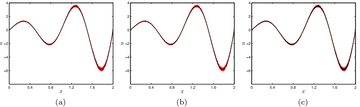
Once the dominant frequency is identified, the corresponding spatial mode is reconstructed via Eq. (10). The mode associated with the main frequency is recovered with a good accuracy even when relying on a drastically reduced subset, see Fig.4where it is plotted as estimated from datasets of different sizes.
The stability of both the DMD and the NU-DMD algorithm under noise corrupting the data is also investigated. The accuracy of the identified dominant frequency when the noise to signal ratio varies is given in TableI. The NU-DMD appears to be very robust with respect to noise and more accurate than DMD in the estimation of the main frequency.
B. Application to a cavity flow
The flow over an open cavity exhibits dynamical features of interest for illustrating our method. The most energetic phenomenon is due to self-sustained oscillations of the impinging mixing layer.18 Such oscillations result from the feedback loop formed, on one hand, by the
Kelvin-Helmholtz vortices convected downstream to the cavity trailing corner, and, on the other hand, by the instantaneous feedback from the pressure field, from trailing to leading edge, induced by the impingement of vortices. As a result, power spectra are organized around a few narrow peaks (most often a single peak at frequency f), with Strouhal numbers f L/U∞close to multiples of 1/2, where
Lis the cavity length andU∞is the incoming velocity.
1. Two-dimensional experimental flow
We first consider an experimental incompressible open cavity flow with aspect ratioL/H=1.5 (depth H=50 mm), Reynolds number Re=U L/ν≃8800, and span-wise aspect ratio of 6. A typical power spectrum, in the configuration of the flow, is shown in Fig.5(b). PIV measurements
FIG. 4. In black, real part of the dominant spatial mode identified by (a) a standard DMD of the whole dataset. (b)
NU-DMD algorithm, withNr/N=5.0×10−2andnp/np=5.0×10
−2. (c) NU-DMD,N
r/N=5.0×10−4,np/np=5.0×10 −4.
TABLE I. Errorϵf=
f−f
/fon the identification of the frequency with a standard DMD applied to theNrfirst snapshots
of the original dataset, and with a NU-DMD applied toNrrandomly selected snapshots, with respect to the noise to signal
ratio.
NSR 5.0×10⁻³ 5.0×10⁻² 5.0×10⁻¹
DMD NU-DMD DMD NU-DMD DMD NU-DMD
Nr/N=0.01 5.2×10⁻⁴ 5.9×10⁻⁵ 1.3×10⁻² 7.3×10⁻⁴ 2.7×10⁻¹ 4.7×10⁻³
Nr/N=0.1 3.6×10⁻⁴ 2.3×10⁻⁵ 2.1×10⁻³ 8.8×10⁻⁵ 3.8×10⁻¹ 2.7×10⁻³
Nr/N=1.0 5.8×10⁻⁵ 3.1×10⁻⁶ 9.1×10⁻⁴ 7.7×10⁻⁵ 4.1×10⁻² 5.8×10⁻⁴
in a vertical (x, y)-plane provide time-resolved 2-D, 2-C velocity fields (see Fig.5(a)for a visuali-zation of the flow in the observation plane). The dataset is formed ofN =5000 fields with a spatial grid ofnp=7018 points.
To illustrate the NU-DMD algorithm,Nrsnapshots taken at random from the full PIV dataset,
hence at random times, are considered. The algorithm is applied to the fluctuating part (zero time-averaged) of this Nr-snapshot dataset. The influence of the number of spatial components
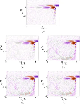
np used in the NU-DMD algorithm is also investigated. The spatial mode associated with the fre-quency of the shear layer from both a standard DMD (N samples uniform in time) and NU-DMD (with varying number of snapshots and retained spatial components) is shown in Fig. 6. When the snapshots are not sampled uniformly in time, the DMD method cannot be applied while the NU-DMD still correctly identifies the flow field dominant modes. Further, very few snapshots are necessary for the dominant features to be accurately identified with this technique since retain-ing only one snapshot among 500 (Nr/N=2.0×10−3 with Nr=10) and one spatial point over
700 (np/np=1.4×10 −3 with
np=10) still results in a decent approximation of the dominant shear-layer mode, see Fig. 6(e). In order to quantify the discrepancy, the absolute value of the relative difference between the amplitude of the NU-DMD and DMD modes is plotted Fig.7for the dominant mode. The modes have been set in phase and the errorϵmodehas been normalized by the
norm of the corresponding component of the DMD mode. The error for theith component is hence defined, in the general case, as
ϵmodei(x, y,z)B
φi,NU-DMD(x, y,z)−φi,DMD(x, y,z)
φi,DMD
2
, i∈{x, y,z}. (19)
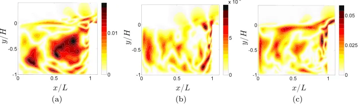
The NU-DMD spatial modes are given by the pseudo-inverse solution Eq. (14) and spatial fields in the null-space ofΛcan then not be resolved. Further, a small frequency differenceδf between, say, the exact dominant frequency and that estimated via NU-DMD will affect the spatial modesM by a contribution associated with that low frequencyδf via Eq. (14). It results that the discrepancy is most visible where the energy of the flow at these low frequencies is large. However, it is seen that it remains below a few percents throughout the spatial domain.
FIG. 5. (a) Snapshot of the flow in the observation plane (vorticity field). (b) Power spectral density of the cavity flow produced by averaging the individual spectra at each spatial points of the velocity field.
FIG. 6. Dominant mode identified by (a) standard DMD (N snapshots ofnp components). (b) NU-DMD algorithm, withNr/N=1.0×10−1andnp/np=1.4×10
−1. (c) NU-DMD,N
r/N=1.0×10−1,np/np=1.4×10
−3. (d) NU-DMD,
Nr/N=2.0×10−3,np/np=1.4×10
−1. (e) NU-DMD,N
r/N=2.0×10−3,np/np=1.4×10
−3. Colors indicate the value
of the vorticity.
The retained spatial points, with their associated cluster supports, are plotted in Fig. 8 for
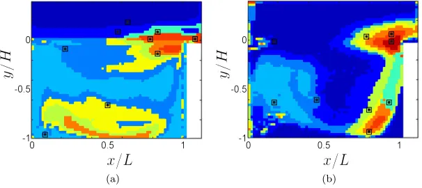
np=10, and in Fig.9fornp=20. As expected, physically relevant areas are discriminated, i.e., the shear-layer, the incoming flow, the flow along the downstream wall, and the inner-flow recircula-tion. Fourier spectra associated with centroids are, by construction, different, see Fig.10where they are plotted for some clusters. The supports of the identified clusters correspond to regions of space where the relative influence of the shear layer (high frequency) and the inner-flow (low frequencies) varies.
The clustering step is robust in the sense that the supports of the identified clusters fornp=10, Fig.8, foliate into smaller and nested supports when np=20, Fig.9. In particular, the topology of the clusters is comparable and no significant new region arises in the clusters support when classifying with a finer description.
FIG. 7. Relative differenceϵmode, see Eq. (19), between the dominant mode identified by a standard DMD and the NU-DMD
algorithm. (a) NU-DMD algorithm, withNr/N=1.0×10−1andnp/np=1.4×10
−1. (b) NU-DMD,N
r/N=1.0×10−1,
np/np=1.4×10−3. (c) NU-DMD,Nr/N=2.0×10−3,np/np=1.4×10
−1. (d) NU-DMD,N
r/N=2.0×10−3,np/np= 1.4×10⁻³.
suboptimal method presented in Sec.III C 3, see Fig.8, hence justifying the proposed suboptimal clustering step scheme as a suitable and relevant proxy for an accurate clustering, robust with respect to the sampling. Our suboptimal method took about 60 s of central processing unit (CPU) time to classify the whole flow field while the minimization of thenpcost functions in Eq. (17) of a
compressed sensing approach would require a very significant computational effort.
The accuracy of the estimation of the dominant frequency f by the NU-DMD algorithm when varying the amount of available information is given in Table IIin terms of relative error
ϵf =|fNU−DMD−fDMD|/fDMD. The quality of the identification of spatial modesφcan be estimated
from the quantification of their main feature, i.e., the amplified travelling waves in the shear layer.
FIG. 8. Illustration of the clustering step proposed in Sec.III C 3.np=10. Black dots indicate spatial components associated
to centroids selected during the clustering process. Colors indicate the different clusters. (a) x-velocity component. (b)
y-velocity component.
FIG. 9. Illustration of the clustering step proposed in Sec.III C 3.np=20. Black dots indicate spatial components associated
to centroids selected during the clustering process. Colors indicate the different clusters. (a) x-velocity component. (b)
y-velocity component.
FIG. 10. x-velocity component power spectral densities associated with the cluster centroids.np=10.
FIG. 11. Fourier-based subset selection. Illustration of the clustering step.np=10. Black dots indicate spatial components
associated to centroids selected during the clustering process. Colors indicate the different clusters. (a)x-velocity component.
TABLE II. Accuracy of the dominant frequency and the wavenumber identification of the shear layer mode by the NU-DMD
algorithm.ϵfB|fNU−DMD−fDMD|/fDMD,ϵκBκNU−1−DMD−κ
−1 DMD
/κ−1
DMD. The DMD is here computed with the maximum
information (Nsnapshots ofnpcomponents) and hence serves as reference.
np/np=0.14 np/np=0.0014
ϵf ϵκ ϵf ϵκ
Nr/N=0.1 8.0×10⁻⁴ 8.0×10⁻³ 3.2×10⁻³ 4.0×10⁻²
Nr/N=0.002 6.9×10⁻⁴ 4.0×10⁻² 6.9×10⁻⁴ 4.1×10⁻²
The main characteristic of these impacting vortices is their wavenumberκ, which can be determined by fitting the velocity profileu(x, y), at some giveny =y0, with the theoretical profile of a spatially
developing instability,
ut h(x, y0)=v0+v1exp(σx)cos(κx+ϕ), (20)
where σ is the spatial growth, ϕ is a reference phase, and {v0,v1} are normalization factors.
It results in identification of the wavenumber by the NU-DMD algorithm with an error ϵκ=
κ−1
NU−DMD−κ −1 DMD
/κ−1
DMDof about 4%, see TableII.
2. Three-dimensional numerical simulation
We now consider the numerical simulation of a three-dimensional incompressible open cavity flow with aspect ratio L/H=2 (depth H=50 mm), Reynolds number Re=U L/ν≃4000 and span-wise aspect ratio of 2, with periodic spanwise boundary conditions. The numerical simulation provides time-resolved three-dimensional (3-D) three-component (3-C) velocity fields (see Fig.12
for a snapshot of the flow in the symmetry(x, y)observation plane. For the sake of readability, colors have been saturated). The dataset is formed ofN=500 snapshots of the velocity field, with a spatial grid of np=2 033 130 points. Details about the numerical simulation can be found in
Ref.16.
The spatially averaged velocity field power spectrum is shown in Fig.13. It exhibits a series of dominant features around a reduced frequency of about 1. In order to assess the applicability and accuracy of the NU-DMD algorithm,Nr=50 (Nr/N =0.1) snapshots of the velocity field are
taken at random from the full DNS dataset, hence at random times. The algorithm is applied to the fluctuating part (zero time-averaged) of thisNr-snapshot dataset. The number of spatial points kept
for the clustering step isnp=100 (np/np=4.9×10 −5).
The main computational bottleneck of the NU-DMD is the identification of the clusters since the classification step in the K-means algorithm (see Sec.III C 2) takes approximately 40 000 s of total CPU time on a desktop computer, and about 4 GB of memory. While the minimization of thenpcost functions in Eq. (17) in a compressed sensing approach would constitute an intractable
computational effort, the evaluation of the central moments in the suboptimal approach proposed in
FIG. 12. Snapshot of the flow in the symmetry plane. Colors encode the velocity field magnitude. (a)x-velocity component.
(b)y-velocity component. (c)z-velocity component. Colors have been saturated in figure (a) in order to make the cavity
internal flow more visible.
FIG. 13. Spatially averaged power spectrum density of the velocity field, from the DNS of the 3-D cavity flow.
Sec.III C 3only requires a few seconds. For illustration and comparison purpose, a DMD using the standard method19,20is also computed. Its evaluation requires over 40 GB of memory and more than 320 000 s of total CPU time. It is hence out-of-reach for a desktop computer and had to be computed on an HPC machine.
The supports of the clusters are plotted in Fig. 14in the(x, y)symmetry plane of the cav-ity. Clusters of the x- and y-components of the velocity field are reminiscent of those of the two-dimensional case discussed in Sec.IV B 1(compare with Fig.8). Both the shear layer and the incoming flow are dynamically well separated (cluster-wise) from the rest of the flow.
Similarly to the two-dimensional case, Sec.IV B 1, dominant DMD modes are associated to oscillations of the shear-layer. The dominant mode, as derived both from the standard DMD algo-rithm and the present NU-DMD approach, is plotted in Fig.15for illustration in terms of isosur-faces of theQ-criterion forQ/(U/L)2∈{1,2}(left) andQ/(U/L)2∈{−1,−2}(right). A very good agreement between the reference, computationally very intensive, DMD method and the NU-DMD approach is observed. A few snapshots, as well as a dramatically reduced number of points in space, are hence sufficient to compute a decent approximation of the dominant DMD mode. The mode associated with the dynamics of the shear layer is plotted in Fig.16in a 2-D plane both from the NU-DMD and the DMD approach. The relative errorϵf B|fNU−DMD−fDMD|/fDMDin the
identifi-cation of the frequency is less than 1.9×10⁻²while the relative errorϵκ=κ−1 DMD−κ
−1 NU−DMD
/κ−1 DMD
in the wavenumber of the shear-layer, evaluated via Eq. (20) as in Sec. IV B 1, is less than 4.4×10⁻³, again illustrating the accuracy of the present method.
In order to quantify the discrepancies between DMD and NU-DMD, the absolute value of the difference between the amplitude of the dominant DMD and NU-DMD mode as defined in Eq. (19) is plotted Fig.17. The modes have been set in phase and the error has been normalized by the norm of the corresponding component of the DMD mode. Differences remain inferior to a few percents and are mainly observed within the cavity for thez-component. As in the 2-D case, patterns typical of inner-flow structures at low frequency are discernible within the cavity on the spatial mode, as
FIG. 14. Illustration of the clustering step introduced in Sec.III C 3.np=100. Colors indicate the different clusters. (a)
FIG. 15. Isosurfaces of positive (left column) and negative (right column)Qcriterion. Top row (respectively, bottom row) corresponds to the DMD (respectively, NU-DMD) dominant shear-layer mode.
FIG. 16. Slice of the dominant mode, identified by a standard DMD (top line, real part of the mode,N snapshots ofnp
components) and the NU-DMD algorithm (bottom line, real part of the mode, withNr/N=0.1 andnp/np=4.9×10
−5).
First, second and last column correspond tox-,y- andz-velocity components respectively. Colors encode the magnitude of
the velocity field.
FIG. 17. Slice of relative differenceϵmode, see Eq. (19), between the dominant mode identified by a standard DMD and the
NU-DMD algorithm. Left, middle and right plots correspond to thex-,y-, andz-velocity component respectively.
discussed in Sec.IV B 1. Further, since thez-component of the velocity fields stored inK is small and carries little energy, the affected part of the mode has a larger relative impact compared to that of the x- and y-component. While not done here, a suitable relative normalization of the different components of the snapshots would balance their contribution to the Frobenius norm in Eq. (12) and result in a better relative accuracy of thez-component.
V. CONCLUSION
We have presented a method for efficiently computing dynamic modes in case of datasets of very large size, where direct computations on the resulting Krylov matrix are out-of-reach, and/or from a system arbitrarily sampled in time, where a standard DMD analysis does not apply. The method essentially formulates the problem in an optimization setting and decouples the estimation of the temporal description from the spatial description. This allows to handle very general datasets, with essentially no restriction on the sampling strategy or the size of the snapshots. With an appro-priate sampling strategy, both very low and very high frequency contents can be retrieved without the need of a large number of snapshots. Further, spatial correlations in space of the observable are exploited to estimate frequencies and growth rates of the dynamic modes from a smaller dataset obtained via a clustering algorithm based on the estimated Fourier spectrum of each component of the spatial field. While the estimation of the dominant Fourier spectra, expected to be compressible, naturally lends itself to a compressed sensing framework, a more computationally friendly imple-mentation relying on statistics of the time series is here used. The effective dataset is small and the resulting NU-DMD method is computationally efficient.
The method has been illustrated on a synthetic flow, exhibiting a 1-D linear instability, and on the experimental dataset of 2-D PIV fields of a 3-D open cavity flow. A large-scale three-dimensional configuration, involving more than 2×10⁶degrees-of-freedom for each snapshot, was
also considered. In all of these cases, spatial modes, frequencies, and growth rates were accurately recovered, even when relying on as low as about 0.1% of the original spatial field and 0.2% of the original snapshots as needed by the standard DMD.
The present NU-DMD method hence constitutes a valuable and widely applicable tool for analyzing physical systems from a dataset of observables with very mild constraints (sampling strategy, missing snapshots, small dataset, etc.).
ACKNOWLEDGMENTS
This work was partially funded by theDigiteo FLUCTUSproject.
1E. Candès and J. Romberg, “Quantitative robust uncertainty principles and optimally sparse decompositions,”Found.
Com-put. Math.6(2), 227–254 (2006).
2E. Candès and T. Tao, “Near-optimal signal recovery from random projections: Universal encoding strategies?,”IEEE Trans.
Inf. Theory52(12), 5406–5425 (2006).
3K. Chen, J. Tu, and C. Rowley, “Variants of dynamic mode decomposition: Boundary condition, Koopman, and Fourier
4J. Ding and A. Zhou,Statistical Properties of Deterministic Systems(Springer, 2010).
5D. Donoho, “Compressed sensing,”IEEE Trans. Inf. Theory52(4), 1289–1306 (2006).
6T. Dreeben and S. Pope, “Probability density function/monte carlo simulation of near-wall turbulent flows,”J. Fluid Mech.
357, 141–166 (1998).
7D. Duke, J. Soria, and D. Honnery, “An error analysis of the dynamic mode decomposition,”Exp. Fluids52, 529–542 (2012).
8A. Gersho and R. Gray,Vector Quantization and Signal Compression(Springer, 1992).
9F. Guéniat, L. Pastur, and F. Lusseyran, “Investigating mode competition and three-dimensional features from
two-dimensional velocity fields in an open cavity flow by modal decompositions,”Phys. Fluids26, 085101 (2014).
10F. Guéniat, L. Pastur, and L. Mathelin, “Snapshot-based flow analysis with arbitrary sampling,” Procedia IUTAM10, 59
(2014).
11M. Jovanovi´c, P. Schmid, and J. Nichols, “Sparsity-promoting dynamic mode decomposition,”Phys. Fluids26(2), 024103
(2014).
12J. C. Lagarias, J. A. Reeds, M. H. Wright, and P. E Wright, “Convergence properties of the Nelder-Mead simplex method
in low dimensions,”SIAM J. Optim.9, 112–147 (1998).
13I. Mezi´c, “Spectral properties of dynamical systems, model reduction and decompositions,”Nonlinear Dyn.41, 309–325
(2005).
14I. Mezi´c, “Analysis of fluid flows via spectral properties of the Koopman operator,”Annu. Rev. Fluid Mech.45, 357–378
(2013).
15V. Pisarenko, “The retrieval of harmonics from a covariance function,”Geophys. J. Int.33(3), 347–366 (1973).
16B. Podvin, Y. Fraigneau, F. Lusseyran, and P. Gougat, “A reconstruction method for the flow past an open cavity,”J. Fluids
Eng.3(128), 531–540 (2006).
17J. Robinson, “A rigorous treatment of ‘experimental’ observations for the two-dimensional Navier-Stokes equations,”Proc.
R. Soc. A457(2008), 1007–1020 (2001).
18D. Rockwell and E. Naudascher, “Self-sustained oscillations of impinging free shear layers,”Annu. Rev. Fluid Mech.11,
67 (1979).
19C. W. Rowley, I. Mezi´c, S. Bagheri, P. Schlatter, and D. S. Henningson, “Spectral analysis of nonlinear flows,”J. Fluid
Mech.641, 115–127 (2009).
20P. Schmid, “Dynamic mode decomposition of numerical and experimental data,”J. Fluid Mech.656, 6–28 (2010).
21P. Schmid, “Application of the dynamic mode decomposition to experimental data,”Exp. Fluids50(4), 1123–1130 (2011).
22A. Seena and J. Sung, “Dynamic mode decomposition of turbulent cavity flows for self-sustained oscillations,”Int. J. Heat
Fluid Flow32(6), 1098–1110 (2011).
23O. Semeraro, G. Bellani, and F. Lundell, “Analysis of time-resolved PIV measurements of a confined turbulent jet using
pod and Koopman modes,”Exp. Fluids53(5), 1203–1220 (2012).
24P. V. Slooten and S. Pope, “Advances in pdf modeling for inhomogeneous turbulent flows,”Phys. Fluids10(1), 246–265
(1998).
25L. Sorber, M. Van Barel, and L. De Lathauwer, “Unconstrained optimization of real functions in complex variables,”SIAM
J. Optim.22(3), 879–898 (2012).
26P. Stoica and T. Soderstrom, “Statistical analysis of music and subspace rotation estimates of sinusoidal frequencies,”IEEE
Trans. Signal Process.39(8), 1836–1847 (1991).
27J. Stoyanov, “Krein condition in probabilistic moment problems,”Bernoulli6, 939–949 (2000).
28F. Takens, “Detecting strange attractors in turbulence dynamical systems and turbulence,”Lect. Notes Math.898, 366–381
(1981).
29J. Tropp and A. Gilbert, “Signal recovery from random measurements via orthogonal matching pursuit,”IEEE Trans. Inf.
Theory53(12), 4655–4666 (2007).
30D. Tufts and R. Kumaresan, “Estimation of frequencies of multiple sinusoids: Making linear prediction perform like
maximum likelihood,”Proc. IEEE70(9), 975–989 (1982).
31Whenever N<
np, the optimization problem (14) may be advantageously substituted with λ∈
arg min λ∈CNmd
R
np(IN−Λ+Λ) F
, withQ npR
np
QR
= K np.