Abstract—With the advent of the Internet of Things, the security of the network layer in the Internet of Things is getting more and more attention. Traditional intrusion detection technologies cannot be well adapted in the complex Internet environment of the Internet of Things. Therefore, it is extremely urgent to study the intrusion detection system corresponding to today's Internet of Things security. This paper presents an intrusion detection model based on improved Genetic Algorithm and Deep Belief Network. Facing different types of attacks, through multiple iterations of the GA, the optimal number of hidden layers and number of neurons in each layer are generated adaptively, so that the intrusion detection model based on the DBN achieves a high detection rate. Finally, the NSL-KDD dataset was used to simulate and evaluate the model algorithm. Experimental results show that the improved intrusion detection model combined with DBN can effectively improve the recognition rate of intrusion attacks and reduce the complexity of the network.
Keywords—Internet of Things security; Intrusion detection; Deep Belief Network; Genetic Algorithm
I. INTRODUCTION
ith the rapid development, Internet of Things (IoT) technology has been widely used, from traditional equipment to common household appliances, which has greatly improved our quality of life [1].
However, IoT systems have become an ideal target of cyber attackers because of its distributed nature, large number of objects and openness [2-5]. In addition, because many IoT nodes collect, store and process private information, they are apparent targets for malicious attackers [6]. Therefore, to maintain the security of the IoT system is becoming a priority of the successful deployment of IoT networks [7].
To detect intruders is one important step in ensuring the security of the IoT networks. Intrusion detection is one of
Submission Date: 2019-02-04
This work was supported by the National Natural Science Foundation of China (no. 61673259).
Ying Zhang*, Ph.D, Professor, he is a faculty of College of Information Engineering, Shanghai Maritime University, Shanghai 201306, China, E-mail: [email protected]
Peisong Li, master student, he studies in the College of Information Engineering, Shanghai Maritime University, Shanghai 201306, China. E-mail: [email protected].
Xinheng Wang, Ph.D, Professor, IEEE Senior Member, he is a faculty of School of Computing & Engineering, University of West London, London W5 5RF, UK, E-mail: [email protected].
*: The correspondent author.
several security mechanisms for managing security intrusions, which can be detected in any of four layers of IoT architecture shown in Fig. 1. The Network Layer not only serves as a backbone for connecting different IoT devices, but also provides opportunities for deploying network-based security defense mechanisms such as Network Intrusion Detection Systems (NIDS) [8].
There are many intrusion detection methods, such as methods based on statistical analysis [9], cluster analysis [10], artificial neural network [11] or deep learning [12]. Among these methods, intrusion detection based on deep learning performs better than other methods [13]. The reason is that deep learning has strong abilities, such as self-learning, self-adaptation, good generalization, and detection against unknown attack behavior.
For the deep learning algorithm, a network structure may have a great detection accuracy for one attack type, but it may not have a good detection effect when facing other attacks. Therefore, we hope to design a self-adaptive model to change the network structure for different attack types, so that our intrusion detection model can maintain a high detection rate continuously.
In the past few years, there has been very little research on the optimization of the IoT intrusion detection model based on deep learning. And, there has not been a unified solution for the selection of the number hidden layer and the number of neurons. Most of the research is based on trial and error and on pruning or constructive methods [14], the network structure and the performance cannot be guaranteed. The random selection of the number of hidden neurons might some problems.
In this paper, a new IoT intrusion detection model is proposed by introducing genetic algorithm into deep belief network to optimize the number of hidden layers and neurons in a hidden layer.
By applying the improved genetic algorithm, for different types of attacks, the optimal number of hidden layers and neurons in a hidden layer can be iteratively generated, and the network complexity can be reduced as much as possible while ensuring the detection rate. The solution of these two problems of deep network can make the intrusion detection system have a greater improvement in performance.
In this paper, we will firstly introduce the related work of intrusion detection based on machine learning in Section II. Then we will introduce the proposed algorithm model in Section III. In Section IV, we show the experimental results and compared it with other methods. This paper is concluded in Section V.
Intrusion Detection for IoT Based on Improved
Genetic Algorithm and Deep Belief Network
Ying Zhang*, Peisong Li and Xinheng Wang
Personalize Information Service
Cloud computing, Intelligence computing
Internet Mobile Communication Network
RFID, Sensor, GPS
Application Layer
Support Layer
Network Layer
Perceptual Layer
Network Security Management
IDS
Fig. 1 IoT architecture
II. RELATED WORK
The intrusion detection technology based on machine learning method can be divided into two major categories: intrusion detection based on artificial neural networks and intrusion detection based on deep learning [15].
Intrusion detection based on artificial neural network is generally divided into three sub-categories of neural networks: supervised, unsupervised and hybrid. The main type of supervised neural networks are multilayer feed-forward (MLFF) neural networks. Ryan et al. [16] used MLFF neural network to detect anomaly based on user behavior. However, supervised neural networks depend on training of a large number of data sets. Sometimes the distribution of training data sets is not balanced, which makes the MLFF neural network easily reach the local minimum value, and thus the stability is low. Detection rate of low-frequency attack is a key factor in judging the quality of the detection model. The detection accuracy of MLFF neural network is low for low-frequency attacks.
The main advantage of the unsupervised artificial neural networks is that new data can be analyzed without tagging data in advance. Yu et al. [17] introduced a theoretical foundation for combining individual detectors with Bayesian classifier combination. This ensemble is fully unsupervised and does not require labeled training data, which in most practical situations is hard to obtain. The Self-Organizing Feature Map (SOM) used in [18] is an unsupervised learning method that extracts features from normal system activity and identifies statistical changes from normal trends. However, for low-frequency attacks, the detection accuracy of unsupervised neural network is also low.
The third category is the hybrid neural network, e.g., FC-ANN proposed in [19] is such a model. The FC-ANN method introduces fuzzy clustering techniques into general artificial neural networks. Using fuzzy clustering techniques, the entire training set can be divided into small, low-complex subsets. Therefore, based on these subsets, the stability of the individual neural network can be improved and the detection accuracy can be improved as well, especially for the detection of low-frequency attacks. Ma et al. [20] proposed a novel approach called SCDNN, which combines spectral clustering (SC) and deep neural network (DNN) algorithms. It provides an effective tool of study and analysis of intrusion detection in large networks. Chiba et al. [21] proposed a cooperative and
hybrid network intrusion detection system (CH-NIDS) to detect the attacks by sensing the network traffic.
In [22], based on Back Propagation neural networks (BPNN), a discussion was made on the selection of the number of hidden layers. It is believed that the training set must be analyzed before the design of the neural network to correctly estimate the similarity between the number of neurons and the number of hidden layers.
At present, there are many intrusion detection technologies based on deep learning. Yin et al. [23] proposed a deep learning approach for intrusion detection using recurrent neural networks (RNN-IDS) which is Suitable for high-precision classification model modeling. Abolhasanzadeh [24] proposed a method for detecting attacks in big data using Deep Auto-Encoder. Gao et al. [25] trained the deep belief network (DBN) as a classifier to detect intrusions. Similarly, Alom et al. [26] also utilized the capabilities of DBN to detect intrusions through a series of experiments.
However, the above articles mainly select the specific network structure through many attempts, and these methods are random and irregular. The selected network structure may not be optimal and suitable for complex network environment.
Compared with traditional neural networks, DBN has the advantages of multi-layer structure and pre-training with fine-tuning learning methods. These advantages enable DBN to extract the deep attributes of training set, thus the problems existing in the traditional neural network intrusion detection methods are solved, such as low training efficiency, easy to fall into the local optimum and the need of large amount of tag data [27].
Many researchers put their effort in analyzing the solution to the problem that how many neurons are kept in the hidden layer in order to obtain the best result. Liu et al. [28] proposed a novel and effective criterion based on the estimation of the signal-to-noise-ratio figure (SNRF) to optimize the number of hidden neurons in the neural networks to avoid overfitting in the function approximation. Rivals and Personnaz [29] used techniques based on least squares estimation and statistical tests for estimating the number of neurons in the hidden layer. Mao and Huang [30] used a data structure preserving (DSP) algorithm to fix the hidden neuron. It is an unsupervised neuron selection algorithm. Doukim et al. [31] proposed a technique to find the number of hidden neurons in an MLP network by using coarse-to-fine search technique, which is applied in skin detection. This technique includes binary search and sequential search. In [32], to fix hidden neurons, 101 various criteria are tested based on the statistical errors. At last the selected
criterion for the NN model is 2 2
(4n +3) / (n −8), where n is the number of input parameters. The results show that the proposed model improves the accuracy and minimal error.
different training types including low-frequency attacks and other types of attacks. The corresponding different network structures are obtained by iterative evolution through GA, thereby detection rate is improved.
III. GA OPTIMIZED DBN MODEL
This paper presents an intrusion detection model by a combined GA and DBN. Through multiple iterations of the GA, an optimal network structure is produced. The network structure contains the number of hidden layers and the number of neurons in each layer. This structure is then applied to deep belief network for intrusion detection.
A. Improved genetic algorithm
Genetic Algorithm is known to be an ideal technique for finding optimal solutions to various problems.
1) Population initialization
The purpose of initialization is to generate an initial population randomly for subsequent genetic manipulation. For a simple training set, up to three hidden layers are enough to get a good detection rate. Binary coding is the most common coding method in genetic algorithm, so we encode the number of nodes in the three hidden layers directly in the binary chromosome. The length of chromosome is 18 bits: the first 6 bits are reserved for the first hidden layer, the subsequent 7-12 bits and 13-18 bits are for the second and the third hidden layers respectively, as shown in Fig. 2:
Fig. 2 Chromosome schematic
A chromosome represents a network structure, which has at most three hidden layers and at least one hidden layer. Each layer has 6 bits. The value of each bit is a binary number 0 or 1. The converted decimal number is the number of neurons in a layer. According to the rules of thumb, it is shown that an acceptable number of neurons in the hidden layer could be the size between the input layer and output layer. Therefore, when the population is initialized, we must ensure that the number of nodes in each layer is smaller than the number of input features and greater than the number of output features.
I≤N≤O (1) where I is the size of the input layer, O is the size of the output layer and Nis the number of neurons in the hidden layer.
If a chromosome has two layers, then 1-6 bits and 7-12 bits are between 000010 and 101000. The 13-18 bits are 000000.
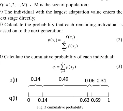
2) Improved selection
The selection operation is to select excellent chromosomes from the current population and prepare for crossover and mutation. As the fitness of candidate individuals increases, the probability of being selected increases. In general, a method of roulette wheel selection based on proportional fitness assignment (also known as Monte Carlo method) is used.
However, one drawback of this method is that the selection based on the generated random number that may lead to some
individuals with high fitness is eliminated. Therefore, we made an improvement: Firstly, we will select the individuals with the greatest fitness value to ensure that they can enter the next stage, and then select the remaining individuals according to the method of roulette. This improvement ensures that the best individuals will not be eliminated.
The specific operations are as follows:
⑴ Calculate the fitness of each individual in the population (i 1, 2, , M)
f = ⋯ ,M is the size of population;
⑵ The individual with the largest adaptation value enters the next stage directly;
⑶ Calculate the probability that each remaining individual is passed on to the next generation:
1 ( ) ( )
( ) i i N
j j
f x p x
f x
= =
∑
(2)
⑷ Calculate the cumulative probability of each individual:
1 ( ) i
i j
j
q p x
=
=
∑
(3)Fig. 3 cumulative probability
⑸ Generate a uniformly distributed pseudo-random number r in the interval [0, 1];
⑹ If r < q(1),select the individual 1,if not,select the individual k when q[k-1]<r≤q[k];
⑺ Repeat ⑷-⑹ M-1 times.
3) Improved crossover
Crossover using partially matched crossover (PMC), the traditional method is to exchange randomly selected segments from two adjacent chromosomes. However, the two adjacent chromosomes, selected by a roulette, are sometimes the same, so two chromosomes remain unchanged after the crossover operation, and thus this crossover operation has no effect. So we take the interval crossover, which is as shown in Eq. 4, for example, if we have n chromosomes, we cross the first one with (n/ 2 1)+ th , the second one with
(n/ 2+2)th, and so on.
c th (n/ 2 ) ,th 1, 2, , / 2
i cross with i i n
= + = … (4)
where c representing the individuals generated after the intersection.
Fig. 4 Crossing chromosomes with different hidden layers
4) Mutation
The mutation operation is to change a certain bit in the chromosome. It can use the random search ability of mutation operator. When the operation result is close to the optimal solution neighborhood, it can quickly converge to the optimal solution.
5) Elite retention strategy
Crossover and mutation may lead to the loss of the optimal individuals in the next generation, and this phenomenon will occur in the evolutionary process frequently. In order to prevent the loss of the best individuals of the current population, which results in that the Genetic Algorithm cannot converge to the global optimal solution, an “elite retention” strategy is introduced in this paper. After each mutation operation, the best individual Α in this generation is compared with the best individual Β that has appeared in the evolution process so far. As shown in Eq. (3), If Β is greater than Α , Β replaces the worst individual in this generation and goes to the next generation, Α goes to the next generation directly. If Α is equal or greater than Β , Α goes to the next generation directly. This process is shown in Eq. 5.
{
, ,A if A B C
Band A if A B
≥ =
< (5) where C represents the one which goes to the next generation.
B. Setting of Fitness function
The goal of our model is to obtain a structure with a high detection rate. Therefore, the selection of the fitness function needs to consider the detection rate of the deep belief network:
corrent 100% all
N P
N
= × (6)
where P represents the detection rate, Ncorrect represents the
number of correctly classified data andNall represents the total
number of data. In this case a network structure with a high detection rate can be retained more easily. At the same time, we also need to consider reducing the number of hidden layers as much as possible on the premise of ensuring the detection rate, because the more layers, the longer the training time will take. In addition to this, under the premise of meeting the accuracy requirements, the structure should be as compact as possible, and the network structure should not be too complicated. Also, experimental results in [23] show that the number of neurons in first and second hidden layers should be kept nearly equal so that the network can be trained easily.
We show the complexity between multiple hidden layers by calculating the standard deviation, σ:
1
1 N ( )2
i
x i
N µ
σ =
−
=
∑
(7)where xi represents the number of neurons in the th
i hidden
layer,µ represents the average of the number of neurons in each layer,and N is the total number of samples.
In order to visually display the complexity, we normalize the standard deviation as:
min max min
σ σ
σ
σ σ
∗ −
=
− (8) So we use the following equation to calculate the fitness function:
f w1 p w2 l w3 (1 σ ) ∗
= × + × + × − (9) where prepresents the detection rate of the current deep belief network, within the range of [0, 1], l is the reciprocal of the number of hidden layers in the network, the smaller the number of hidden layers, the larger the reciprocal value is, and the range is [0, 1]. σ∗ is the standard deviation after normalization, within the range of [0, 1]. And f is the fitness value, and should be within the range [0, 1]. w1, w2and w3 are weights.
After continuous testing, we finally take w1=0.995 ,
2 0.005
w = and w3=0.005.
f 0.99 p 0.005 l 0.005 (1 σ∗)
= × + × + × − (10)
By using Eq. 10, individuals with higher detection rates, fewer hidden layers and smaller complexity can be more easily retained, so we can obtain structures with high detection rates, few hidden layers and low complexity easily.
The improved GA flow chart is shown in Fig. 5:
Fig. 5 improved GA flow chart
C. Restricted Boltzmann Machines
pre-processed data, processing and abstracting high-dimensional data [33].
1) Parameter learning
In RBM, v represents all visible units and h represents all hidden units. To determine the model, we only need to obtain three parameters of the model: θ = {W, A, B}.There are weight matrix W, visible layer element bias A and hidden layer element bias B, respectively.
Suppose an RBM has n visible cells and m hidden cells, vi
represents the ith visible unit, i
h represents the jth hidden unit,
and its parameter form is:
{ , }
n m i j
W w R×
= ∈ (11)
wherewi j, represents the weight between the ith visible cell
and the jth hidden cell;
{ m} i
A= a ∈R (12)
whereai represents the bias threshold of the ith visible cell;
{ n} j
B= b ∈R (13)
wherebj represents the bias threshold of the th
j visible cell.
For a set of ( , )v h under a given state, assuming that both visible and hidden layer obey Bernoulli distribution, the energy formula of RBM is:
1 1 1 1
( , | )
n m n m
i i j j i ij j
i j i j
E v h θ a v b h v W h
= = = =
= −
∑
−∑
−∑ ∑
(14)where, θ={W a bij, ,i j} is a parameter of the RBM model, and the energy function indicates that there is an energy value between the value of each visible node and that of each hidden layer node.
After the exponential and regularization of the energy function, the joint probability distribution formula can be obtained that the node set of visible layer and the node set of hidden layer are in a certain state respectively ( , )v h :
( , | )
( , | )
( ) E v h
e P v h
Z
θ
θ
θ
−
= (15)
( , | ) ,
( ) E v h
v h
Z θ e− θ
=
∑
(16)Where, Z( )θ is a normalized factor or partition function, representing the sum of the energy exponents of all possible states of the node set of the visible layer and the hidden layer.
The derivation of likelihood function is often used to get the parameters. Given the joint probability distribution ( , | )P v h θ ,
the marginal distribution ( | )P v θ of the node set of the visible layer can be obtained by summation over all states of the hidden layer node set:
( | ) 1 ( , | )
( )
E v h
h
P v e
Z
θ
θ θ
−
=
∑
(17)Marginal distribution represents the probability that the set of nodes in the visible layer is in a certain state distribution.
Due to the special layer-layer connection and inter-layer connectionless structure of RBM model, it has the following important properties:
① Given the state of the visible cell, the activation states of each hidden layer cell are conditionally independent. At this time, the activation probability of the jth hidden element is:
( j 1| ) ( j i ij) i
P h = v =σ b +
∑
v W (18)② Correspondingly, when the state of the hidden element is given, the activation probability of the visible element is also conditional independent:
( i 1| ) ( i ij j) j
P v = h =σ a +
∑
W h (19)where, ( )σ x is the sigmoid function.
2) solving parameters
To determine RBM model, it is necessary to solve the three parameters of the model: θ={W a bij, i, j}.
The parameter solution uses the logarithmic likelihood function to take the derivative of the parameter.
As we know from ( | ) 1 ( , | )
( )
E v h
h
P v e
Z
θ
θ θ
−
=
∑
, energy E isinversely proportional to probability P, and E is minimized by maximizing P.
The common method to maximize the likelihood function is the gradient rise method, which refers to the modification of parameters according to the following formula:
θ θ µ ln ( )P v θ
∂
= +
∂ (20)
This iteration maximizes the likelihood function P and minimizes the energy E.
The format of logarithmic likelihood function: ln ( )P vs , vs represents the input data of the model, and a single sample is first analyzed here, that is, s
v is the th
s sample in the data set. Then take the derivatives of the parameters in {W a bij, i, j}
respectively:
,
ln ( )
( 1 | ) ( ) ( 1 | )
s
s s
i j i j
v i j
P v
P h v v P v P h v v
w
∂
= = − =
∂
∑
(21)ln ( ) ( ) s s i i v i P v
v P v v
a
∂
= −
∂
∑
(22)ln ( ) ( 1 | ) ( ) ( 1 | )
s s i i v i P v
P h v P v P h v
b
∂
= = − =
Since the second term of the above three equations contains P(v), P(v) still contains parameters, so we solve it by Gibbs sampling.
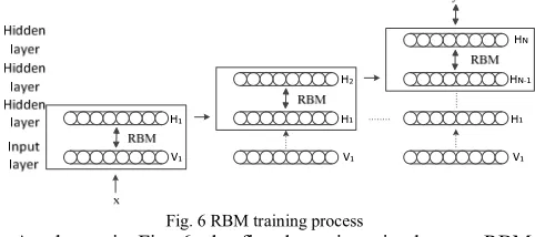
D. DBN for intrusion detection
DBN module is mainly divided into two steps in the training phase:
(1) Each RBM is trained separately, characterized by unsupervised and independent, to ensure that feature information is retained as much as possible when mapping feature vectors into different feature spaces.
In training a single RBM, weight updates are performed with gradient descent via the following equation:
ij(t 1) ij(t) log( ( )) ij
p v
w w
w
η∂
+ = +
∂ (24)
where p v( ) is the probability of a visible vector, which is given by:
( , ) 1
( ) E v h h
p v e
Z
−
=
∑
(25)Z is the partition function (used for normalizing) and E v h( , ) is the energy function assigned to the state of the network.
The observed joint distribution of the input value xand hidden layerHkis modeled as follows:
2
1 1 1
0
( , , , ) ( ( | )) ( , )
N
N k k N N
k
P x H H P H H P H H
−
+ −
=
=
∏
… i (26)
where x=H0 , P H( k−1|Hk) is a conditional distribution of
visible units in theklayer with the condition of hidden units of RBM. P H( N−1,HN) is the visible-hidden joint distribution at
the top level of the RBM. This process is illustrated in Fig. 6.
Fig. 6 RBM training process
As shown in Fig. 6, the first layer is trained as an RBM, assigning thex input toV1as the visible layer.
The input data obtained from the first layer is characterized as the second layer’s data. Two ways exist, average activation
1 0
( 1 | )
P H = H or sample P H( 1|H0).
Once an RBM is trained, another RBM is "stacked" atop it, taking its input from the final trained layer. The new visible layer is initialized to a training vector, and values for the units in the already-trained layers are assigned using the current weights and biases. The new RBM is then trained with the procedure above. This whole process is repeated until the desired stopping criterion is met [34].
Finally, this process is repeated until to the last layer. This is a Deep Learning method.
(2) The last layer of the DBN is the BP neural network. The feature vector of upper RBM is used as an input vector to train
an entity classifier under supervision. Since the RBM of each layer can only ensure its own weight corresponding to the feature vector is optimal after the first step training, our ultimate goal is to make the overall weight corresponding to the feature vector as optimal. So according to the characteristics of the BP neural network, the BP neural network can propagate error information from the top layer to the bottom layer of RBM. If fine-tune the DBN network is finely tuned, a global optimization could be achieved.
The number of hidden layers and the number of neurons in each layer in the deep belief network are determined by the algorithm model we constructed earlier.
E. Algorithm flow
The algorithm flow is summarized as:
Step1: Initialize the population and generate different number of hidden layers and the number of neurons in each layer randomly;
Step2: Calculate the fitness value according to Eq. 8, chosen by the roulette method, and keep the optimal individual in the present; interval crossover; variation;
Step3: "Elite" retains, retaining individuals with the greatest fitness value during evolution;
Step4: Determine if the maximum number of iterations has been reached. If reached, the generated network structure is retained, otherwise iterate Step2- Step3 again;
Step5: Use the optimal network structure for the deep belief network and train the intrusion detection model.
Step6: Classify the testing set by the trained DBN module, and finally match the classification result with the category information of the testing set to check the accuracy of the classification.
Backward propagation
Restricted Boltzmann Machines, RBM
Backward propagation network,BP
Standard tag information
Output data (Intrusion detection results)
N selection
crossover
mutation
“Elite”
retention
Maximal genetic algebra? Start
End Optimal network structure Y Input data
According to the results, the network
structure is constantly optimized.
Fig. 7 Algorithm model flow chart
The pseudocode of the algorithm is expressed as follows:
Algorithm: Intrusion Detection Model
--f1 : the individual with greatest fitness value in this generation --fbest :the best individuals that emerged during evolution --L : the number of hidden layers
--N : the number of nodes in every hidden layer 1: Initialization
2: Calculate the fitness value of initial population
3: f 0.99 p 0.005 l 0.005 (1 σ ) ∗
= × + × + × −
4: for I from 1 to 50 5: selection 6: crossover 7: mutation
8: calculate the fitness value 9: find out the individual f1 10: compare with the 1f and thefbest 11: if f1> fbest
12: fbest← f1
13: keepf1in the next iteration 14: else
15: keepf1in the next iteration 16: set fbestin the next iteration
17: dalete the one with smallest fitness value 18: end if
19: if I = 50 20: broadcast fbest
21: get theLandNfromfbest 22: end if
23: end for 24: for I from 1 to L
25: training the th
I RBM 26: end for
27: Training the BP, fine-tune the RBM 28: Test DBN with test set
IV. EXPERIMENTAL SIMULATION
A. Experimental data
KDDCUP99 [35] and NSL-KDD are the most commonly used datasets in the intrusion detection research. We used NSL-KDD intrusion dataset which is available in csv format for model validation and evaluations. The dataset composes of the attacks shown in Table 1, and identified as a key attack in IoT computing. Sherasiya and Upadhyay (2016) point out that IoT objects are also exposed to such types of attacks. Furthermore, Sherasiya and Upadhyay (2016) point out that the data that IoT objects exchange are of the same value and importance, or occasionally more important than a non-IoT counterpart [36].
According to the analysis of KDDCUP99 and its latter version NSL-KDD, malicious behaviors (attacks) in network-based intrusions can be classified into the following four main categories:
Probe: when an attacker seeks to only gain information about the target network through network and host scanning activities.
DoS (denial of service): when an attacker interrupts legitimate users’ access to the given service or machine. U2R (User to Root): when an attacker attempts to escalate a
limited user’ privilege to a super user or root access (e.g. via malware infection or stolen credentials).
R2L (Remote to Local): when an attacker gains remote access to a victim machine imitating existing local users.
TABLE I
The attacks in NSL-KDD dataset
Main class Sub class (attacks)
in train set
New sub class (attacks) in test set
DoS Back, land,
Neptune, Smurf, pod, teardrop
Apache2, Mailbomb, Processtable
Probe Imap, multhop,
phf, spy, warezclient, warezmaster, ftp write, guess passwd
Mscan, Saint
U2R Buffer overflow,
perl, loadmodule, rootkit
Httptunnel, Ps, Sqlattack, Xterm
R2L Ipsweep, nmap,
portsweep, satan
Sendmail, Named, Snmpgetattack, Snmp guess, Xlock, Xsnoop, Worm
algorithm in detecting unknown or uncommon attacks. The original dataset consists of 125,973 records of train and 22,544 records of test, each with 41 features such as duration, protocol, service, flag, source bytes, destination bytes, etc. The traffic distribution of NSL-KDD dataset is shown as in the Table 2.
TABLE II
The traffic distribution of NSL-KDD dataset
Traffic Training test
Normal 67343 9711
DoS 45927 7458
Probe 11656 2754
R2L 995 2421
U2R 52 200
Total 125973 22544
In order to make the classification result more accurate and meet the standard conditions of the DBN’s input data set, the data set needs to be normalized. Normalization techniques are necessary for data reduction since it is quiet complex to process huge amount of network traffic data with all features to detect intruders in real time and to provide prevention methods. The method used in this paper is the Min-Max normalization method, also known as deviation standardization, which is a linear change to the original data, mapping the resulting value to [0, 1], the conversion function is as follows:
* X Min
X
Max Min
− =
− (27) where Max is the maximum value of the sample data, and Min is the minimum value of the sample data.
Below is a summary of the metrics we adopted to evaluate the detection method:
Predicted: normal Predicted: attack
Actual:normal TN FP
Actual:attack FN TP
TP TN
ACC
TP TN FP FN
+ =
+ + +
TP DR
TP FN
= +
FP FAR
TN FP
= +
TP Precision
TP FP
= +
( )
TP Recall
TP FN
= +
where, accuracy (ACC) is the percentage of true detection over total data instances; detection rate (DR) represents ratio of intrusion instances; false alarm rate (FAR) represents the ratio of misclassified normal instances; Precision represents how many of the returned attacks are correct; Recall represents how many of the attacks does the model return.
FP: false positive, TP: true positive, TN: true negative, FN: false negative.
B. SIMULATION ENVIRONMENT
The experiment was conducted using MATLAB R2016a running on a personal computer (PC). GA optimized DBN model is trained with the training sets and then evaluated using the test set.
C. SIMULATION RESULTS
First, we need to set the number of generations of the genetic algorithm.
fi
tn
e
s
s
v
a
lu
e
Fig. 8 Genetic algorithm iterative results
It can be seen from Fig. 8 that as the number of iterations increases, the fitness value increases, and when the number of iterations exceeds 50, the curve tends to be stable, and the fitness value no longer increases with the number of iterations. Therefore, we set the genetic algebra of the genetic algorithm to 50 generations.
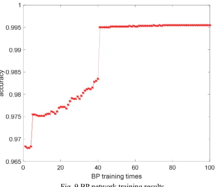
Secondly, set the training times for the BP network.
a
c
c
u
ra
c
y
Fig. 9 BP network training results
From Fig. 9, we can see that when the number of training exceed 80 times, the curve is basically stable, and with the increase in the number of training, the classification accuracy rate no longer increases significantly and wasted training time in vain, so we set the BP network training epochs to 80.
a
c
c
u
ra
c
y
Fig. 10 RBM training results
From Fig. 10 we can see that the training times of RBM have little effect on the classification accuracy rate, there is no obvious increase or decrease trend, so we set the RBM training epochs to 10.
Finally, we use DoS, R2L, Probe, U2R four classes of attacks as intrusion attack training sets respectively. Through an improved genetic algorithm, the optimal network structure for each type of attack is obtained, the iterative process for each type of attacks is shown in Fig. 11:
0 10 20 30 40 50
generations
0.97 0.975 0.98 0.985 0.99 0.995
DoS R2L Probe U2R
Fig. 11 Iterative results with different attacks
We decode the optimal chromosome generated by the iteration, and then get the optimal network structure as shown in Table 3:
TABLE III
Optimal network structure for different types of attacks
Number Attack Network Structure
A DoS 41-18-12-2
B R2L 41-31-2
C Probe 41-26-2
D U2R 41-38-2
The network structure of the deep neural network includes the input layer, hidden layer, and output layer. Because each record in the data set has 41 features, the size of input layer is 41; the output has two characteristics: normal and abnormal, so
the size of output layer is 2. The middle is hidden layer. For data sets with different attack types, the different optimal network structure is generated by multiple iterations of the genetic algorithm. For example, shown in table 1, if DoS is used as a training set, the optimal network structure obtained is A, the structure is 41-18-12-2.
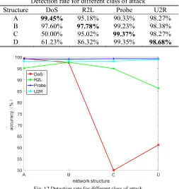
Intrusion detection is performed on four classes of attacks using the A-D network structures respectively, and their detection rates are calculated. Shown in table 4:
TABLE IV
Detection rate for different class of attack
Structure DoS R2L Probe U2R
A 99.45% 95.18% 90.33% 98.27%
B 97.60% 97.78% 99.23% 98.38%
C 50.00% 95.02% 99.37% 98.27%
D 61.23% 86.32% 99.35% 98.68%
a
c
c
u
ra
c
y
(
%
)
Fig. 12 Detection rate for different class of attack
It can be seen from Fig. 12, for a certain type of network structure generated by the certain type of attack, the detection rate of this type of network is higher than other network structures. For example, shown in Fig. 12, the DoS detection rate of network structure A generated by DoS as a training set is significantly higher than that of other structures; the R2L detection rate of network structure B generated by R2L as a training set also significantly higher than that of other structures. The classification accuracy of Probe and U2R is relatively high under all the four network structures, so the comparison results are not very significant. It can be seen that the network structure adaptively generated by the genetic algorithm has a higher detection rate than other network structures.
At the same time, we compared our method with the methods TANN, FC-ANN, SA-DT-SVMS, and BPNN proposed by others. Because all four methods use the KDDCUP99 data set, the test results are comparative. The results obtained are compared with the above methods and summarized in the following table:
TABLE V
Classification accuracy of each method
Method DoS R2L Probe U2R
TANN 90.94% 80.53% 94.89% 60.00%
SA-DT-SVMS 100.00% 93.22% 98.36% 80%
BPNN 80.35% 89.12% 89.12% 25.58%
GA-DBN 99.45% 97.78% 99.37% 98.68%
a
c
c
u
ra
c
y
(
%
)
Fig. 13 classification accuracy of each method
It can be seen from Fig. 13 that the proposed GA-DBN method has reached a very high level for the detection of four types of attacks. The classification accuracy of DoS is higher than 99%, and the classification accuracy of R2L, Probe and U2R is also significantly higher than other methods.
The performances of detecting different attack in the following table:
TABLE VI
The traffic distribution of NSL-KDD dataset ACC
(%) DR
(%) FAR
(%)
Precision
(%)
Recall
(%)
DoS 99.45 99.7 0.8 99.20 99.7
Probe 99.37 99.4 0.7 99.30 99.4
R2L 97.78 93.4 7.3 92.75 93.4
U2R 98.68 98.2 1.8 98.20 98.2
V. CONCLUSION
Through GA, the optimal individuals can be generated. DBN can effectively process high complex and high dimensional data, and the classification results are very good. So in this paper, the improved genetic algorithm combined with a deep belief networks, GA performs multiple iterations to produce an optimal network structure, DBN then uses the obtained network structure as an intrusion detection model to classify the attacks. In this way, facing different attacks, the problem of how to select an appropriate network structure when using deep learning methods for intrusion detection is solved, and thus it improves the classification accuracy and generalization of the model, and reduces the complexity of network structure.
This method has many advantages: on the one hand, the specific network structure generated for specific attack types is higher in classification accuracy than other network structures, which can reach more than 99%. On the other hand, for small training sets, such as U2R, the classification accuracy of our
algorithm is also significantly higher than other methods. In addition, as the model complexity is reduced, the training time of DBN can be reduced without affecting the accuracy of model classification.
In addition, the algorithm combining GA and DBN model not only can be used in intrusion detection in the IoT, also can be applied to other situations, such as classification and recognition. For different training sets, an optimal network structure is adaptively generated for classification. Moreover, for small training sets, high classification accuracy can also be achieved, which helps to find low-frequency attacks in intrusion detection systems. In the future, we will consider to optimize the other parameters of the deep network, reduce the training time and improving the accuracy.
REFERENCES
[1] Q. Jing, A. V. Vasilakos, J. Wan, J. Lu, and D. Qiu, “Security of the Internet of Things: perspectives and challenges,” Wireless Networks, vol. 20, pp. 2481–2501, 2014.
[2] A. Abduvaliyev, A.K Pathan, J. Zhou, R. Roman and W. Wong, “On the
Vital Areas of Intrusion Detection Systems in Wireless Sensor Networks”, Communications Surveys & Tutorials, IEEE vol. 15, pp. 1223-1237, 2013.
[3] S. Sicari, A. Rizzardi, L. A. Grieco, and A. Coen-Porisini, “Security, privacy and trust in internet of things: The road ahead,” Computer Networks, vol. 76, pp. 146–164, 2015.
[4] M. Farooq , M. Waseem , A. Khairi , and S. Mazhar , "A Critical Analysis on the Security Concerns of Internet of Things (IoT),” Perception, vol. 111, pp. 1-6, 2015.
[5] Tuhin Borgohain, Uday Kumar, Sugata Sanyal, “Survey of Operating Systems for the IoT Environment”, arXiv preprint arXiv:1504.02517, vol. 6, pp. 2479-2483, 2015
[6] H HaddadPajouh, A Dehghantanha, R Khayami, KK Choo, “A deep
Recurrent Neural Network based approach for Internet of Things malware threat hunting”, Future Generation Computer Systems, vol. 85, pp. 88–96, 2018.
[7] M Conti, A Dehghantanha, K Franke, S Watson, “Internet of Things Security and Forensics: Challenges and Opportunities”, Elsevier Future Generation Computer Systems Journal, vol. 78, pp. 544-546, 2017.
[8] H. H. Pajouh, R. Javidan, R. Khayami, D. Ali, and K. K. R. Choo, “A
two-layer dimension reduction and two-tier classification model for anomaly-based intrusion detection in iot backbone networks,” IEEE Transactions on Emerging Topics in Computing, vol. PP, no. 99, pp. 1–1, 2016.
[9] W. Lee and S. J. Stolfo. Data mining approaches for intrusion detection. In Proceedings of the 7th USENIX Security Symposium, San Antonio, TX, pp. 120–132, January 1998.
[10] L. Khan, M. Awad, and B. M. Thuraisingham. A new intrusion detection
system using support vector machines and hierarchical clustering. VLDB J., 16(4):507–521, 2007.
[11] E. Hodo, X. Bellekens, A. Hamilton, P. L. Dubouilh, E. Iorkyase, C. Tachtatzis, and R. Atkinson, “Threat analysis of iot networks using artificial neural network intrusion detection system,” in 2016
International Symposium on Networks, Computers and
Communications (ISNCC), May 2016, pp. 1–6.
[12] A. Diro and N. Chilamkurti, ‘‘Distributed attack detection scheme using deep learning approach for Internet of Things,’’ Future Generat. Comput. Syst., vol. 282, pp. 761–768, May 2017.
[13] R. Beghdad, “Critical study of neural networks in detecting intrusions,” Computers and Security, vol. 27, pp. 168-175, 2008.
[14] S. Mukkamala, G. Janoski, and A. Sung. “Intrusion detection using neural networks and support vector machines,” Proceedings of the International Joint Conference on Neural Networks (IJCNN’02), Honolulu, HI, USA, pp. 1702–1707, 2002.
[15] E. Hodo, X. J. A. Bellekens, A. Hamilton, C. Tachtatzis, and R. C. Atkinson, “Shallow and deep networks intrusion detection system: A taxonomy and survey,” CoRR, vol. abs/1701.02145, 2017.
networks,” in Proc. Advances NIPS 10, Denver, CO, pp. 943–949, 1997.
[17] E. Yu, and P. Parekh, “A Bayesian Ensemble for Unsupervised Anomaly
Detection,” in arXiv preprint arXiv:1610.07677, pp. 1–5, 2016.
[18] A Saraswati, M Hagenbuchner, Zhi Quan Zhou, “High Resolution SOM
Approach to Improving Anomaly Detection in Intrusion Detection Systems”, Carcinogenesis, vol.9992, pp.947-954, 2016.
[19] G. Wang, J. Hao, J. Ma, L. Huang, “A new approach to intrusion detection using artificial neural networks and fuzzy clustering”, Exp. Syst. Appl. pp. 6225–6232, 2010.
[20] T Ma, F Wang, J Cheng, Y Yu, and X Chen, "A hybrid spectral clustering and deep neural network ensemble algorithm for intrusion detection in sensor networks," in Sensors vol. 16, no. 10, 2016.
[21] Z Chiba, N Abghour, K Moussaid, and M Rida, "A cooperative and hybrid network intrusion detection framework in cloud computing based on snort and optimized back propagation neural network," in Procedia Computer Science vol. 83 pp. 1200-1206, 2016.
[22] S. Karsoliya. “Approximating number of hidden layer neurons in
multiple hidden layer BPNN architecture,” International Journal of Engineering Trends and Technology, vol.3, pp. 713–717, 2012.
[23] C Yin, Y Zhu, J Fei, and X He, "A deep learning approach for intrusion detection using recurrent neural networks," in IEEE Access vol. 5 pp. 21954-21961, 2017.
[24] B. Abolhasanzadeh, “Nonlinear dimensionality reduction for intrusion detection using auto-encoder bottleneck features,” in 2015 7th Conference on Information and Knowledge Technology (IKT), Urmia, Iran, pp. 1–5, 2015.
[25] N. Gao, L. Gao, Q. Gao, and H. Wang, “An Intrusion Detection Model
Based on Deep Belief Networks,” in 2014 Second International Conference on Advanced Cloud and Big Data, Huangshan, China, pp. 247–252, 2014.
[26] M. Z. Alom, V. Bontupalli, and T. M. Taha, “Intrusion detection using
deep belief networks,” in 2015 National Aerospace and Electronics Conference (NAECON), Dayton, Ohio, USA, pp. 339–344, 2015.
[27] Q. Tan, W. Huang, and Q. Li, “An intrusion detection method based on
DBN in ad hoc networks,” in International Conference on Wireless Communication and Sensor Network, Wuhan, China, pp. 477–485,
2016.
[28] Y. Liu, J. A. Starzyk, and Z. Zhu, “Optimizing number of hidden neurons in neural networks,” in Proceedings of the IASTED International Conference on Artificial Intelligence and Applications (AIA ’07), Innsbruck, Austria, pp. 121–126, February 2007.
[29] I. Rivals I. and L. Personnaz, “A statistical procedure for determining the optimal number of hidden neurons of a neural model,” in Proceedings of the Second International Symposium on Neural Computation (NC’2000), Berlin, May, 23-26, 2000.
[30] K. Z. Mao and G. B. Huang, “Neuron selection for RBF neural network
classifier based on data structure preserving criterion,” IEEE Transactions on Neural Networks, vol. 16, no. 6, pp. 1531–1540, 2005.
[31] C. A. Doukim, J. A. Dargham, and A. Chekima, “Finding the number of
hidden neurons for an MLP neural network using coarse to fine search technique,” in Proceedings of the 10th International Conference on Information Sciences, Signal Processing andTheir Applications (ISSPA ’10), pp. 606–609,May, 2010.
[32] K.G. Sheela, S.N. Deepa, “Review on methods to fix of hidden neurons
in neural networks”, Mathematical Problems in Engineering, vol. 2013, 2013.
[33] G. E. Hinton, S. Osindero, and Y. Teh, “A fast learning algorithm for deep belief nets,” Neural Computation, vol. 18, pp. 1527–1554, 2006.
[34] Y. Bengio, “Learning deep architectures for AI,” Foundat. and Trends Mach. Learn., vol. 2, no. 1, pp. 1–127, 2009.
[35] M. Tavallaee, E. Bagheri, W. Lu, and A. Ghorbani, “A Detailed Analysis
of the KDD CUP 99 Data Set,” Submitted to Second IEEE Symposium on Computational Intelligence for Security and Defense Applications (CISDA) , Ottawa, ON, 2009.
[36] A, Alghuried, “A Model for Anomalies Detection in Internet of Things
![TABLE VI [6]The traffic distribution of NSL-KDD dataset](https://thumb-us.123doks.com/thumbv2/123dok_us/984940.1598123/10.595.41.293.83.331/table-vi-traffic-distribution-nsl-kdd-dataset.webp)
