R E S E A R C H
Open Access
Image segmentation algorithm by piecewise
smooth approximation
Yan Wang
1*and Chuanjiang He
2Abstract
We propose a novel image segmentation algorithm using piecewise smooth (PS) approximation to image. The proposed algorithm is inspired by four well-known active contour models, i.e., Chan and Vese’piecewise constant (PC)/smooth models, the region-scalable fitting model, and the local image fitting model. The four models share the same algorithm structure to find a PC/smooth approximation to the original image; the main difference is how to define the energy functional to be minimized and the PC/smooth function. In this article, pursuing the same idea we introduce different energy functional and PS function to search for the optimal PS approximation of the original image. The initial function with our model can be chosen as a constant function, which implies that the proposed algorithm is robust to initialization or even free of manual initialization. Experiments show that the proposed algorithm is very appropriate for a wider range of images, including images with intensity inhomogeneity and infrared ship images with low contrast and complex background.
Keywords:Image segmentation, Active contour model, Piecewise smooth approximation, Level set method, Partial differential equation
Introduction
Image segmentation is a popular problem in image pro-cessing and computer vision, which has been studied ex-tensively in past decades. The segmentation goal is to separate image domain into a collection of distinct regions, upon which other high-level tasks such as objects recognition and tracking can be further performed. Due to the presence of noise, complex background, low intensity contrast with weak edges, and intensity inhomogeneity [1], image segmentation is still a difficult problem in prac-tical applications, especially for traditional segmentation methods [2-8]. Traditional methods, like Canny edge de-tection [7], are simple and fast, but they always need fur-ther edge linking operation to produce continuous object boundaries [9]. To address these issues, more recent methods including implicit active contours [9-17] have been developed for image segmentation.
Implicit active contours are active contour models imple-mented via the level set method [18]. One of the remark-able advantages of active contour models is that it can
provide smooth and closed contours, which is generally impossible in traditional segmentation methods. Existing implicit models can roughly be categorized into two classes: edge-based models [10,11,13] and region-based models [12,14-16]. Edge-based models use local edge infor-mation (image gradient) to perform contour extraction, which are usually to noise and weak edges. Region-based models utilize the global and/or local image statistics inside and outside the active contour (evolving curve) to find a partition of image domain. They generally have better per-formance in the presence of weak or discontinuous bound-aries and less sensitive to initialization.
A major category of the region-based level set methods is proposed to minimize the well-known Mumford and Shah (MS) functional [19]. Due to the difficulty of directly minimizing the MS functional, different approximation methods have been proposed to allow more efficient en-ergy minimization. For example, the piecewise constant (PC) models [12,20] approximate image domain by a set of homogenous regions, but which is not true for images with intensity inhomogeneity. In [21,22], more advanced piece-wise smooth (PS) models have been proposed to improve the PC model performance in terms of intensity inhomo-geneity. However, due to rather complicated algorithms, * Correspondence:[email protected]
1
College of Mathematics, Chongqing Normal University, Chongqing 401331, China
Full list of author information is available at the end of the article
these models are usually computationally expensive. As indicated in [23], the models using global image statistics usually have difficulty to segment many real-world images with intensity inhomogeneity.
To address this issue, recently localized region-based models [14,16,23-25] have been proposed. For example, Li et al. [14] proposed a region-scalable fitting (RSF) model (originally termed as local binary fitting (LBF) model [26]), which draws upon spatially varying local region informa-tion and thus is able to deal with intensity inhomogeneity. The RSF model has better performance than PC and PS models in segmentation of accuracy and computational ef-ficiency. However, since there are totally four convolutions to be computed at each iteration in the implementation, the RSF model is still computationally expensive. For more efficient segmentation, Zhang et al. [16] proposed a novel active contour model driven by local image fitting (LIF) en-ergy. The LIF energy is constructed by the local image in-formation, which can be viewed as a constraint of the differences between the fitting image and the original image. The complexity analysis and experimental results show that this model is more efficient than the LBF model, while yielding similar results.
These localized methods [14,16,25,26] are, however, to some extent sensitive to contour initialization. Since the segmentation results typically depend on the selection of initial contours, these methods need user intervention to define the initial contours professionally. This means that they may be fraught with the problems of how and where
to define the initial contours. The multiple-seed
initialization used by Vese and Chan [21] also cannot
al-ways produce better results than the single-seed
initialization [27]. Therefore, it is still a great challenge to find an efficient way to tackle the initialization problem.
In this article, inspired by the above-mentioned four models [Chan–Vese (CV), PS, RSF, and LIF models], we propose a novel image segmentation algorithm without ini-tial contours using PS approximation. The four models share the same algorithm structure to find a PC/smooth approximation to the original image; the main difference is how to define the energy functional to be minimized and the PC/smooth function. Pursuing the same idea, in this study, we introduce different energy functional and PS functions to search for the optimal PS approximation of the original image. In the proposed algorithm, the initial function can be chosen as a constant function, which im-plies that the proposed algorithm allows for robustness to initialization or even free of manual initialization. Experi-ments show that the proposed algorithm works well for images with intensity inhomogeneity. Moreover, it is very appropriate for infrared images with low contrast and com-plex background.
The remainder of this article is organized as follows. In “Related studies” section, we briefly review several
classical region-based models and indicate their limita-tions. The proposed algorithm is introduced in“The LIF model results in a local fitted image” section. The pro-posed model presents experimental results using a set of synthetic and real images. This article is summarized in
“Experimental results”section.
Related studies
Chan–Vese (CV) PC models
Chan and Vese [12] restricted the MS minimal partition problem [19] to PC functions and proposed a technique that implements efficiently the PC MS model via level set methods [18]. In level set methods, a contour C is represented implicitly by the zero-level set of a Lipschitz function ϕ:Ω!R, which is called a level set function. In what follows, we let the level set functionϕtake posi-tive and negaposi-tive values inside and outside the contour C, respectively.
Let I:Ω⊂R2!R be an input image and H be the
Heaviside function, the energy functional of the CV model is defined as:
ECVðc
1;c2;ϕÞ ¼λ1 Z
ΩjIc1j 2
HðϕÞdxþλ1 Z
ΩjIc2j 2
ð1HðϕÞÞdxþν
Z
ΩjrHð Þϕjdx ð1Þ
where λ1;λ2>0 , v> 0 are constants. c1 and c2are the global averages of the image intensities in the region
x:ϕð Þx >0
f g andfx:ϕð Þx <0g, respectively, which
are defined as:
c1ð Þ ¼ϕ Z
ΩZI xð ÞHðϕð Þx Þdx
ΩHðϕð Þx Þdx
;c2ð Þϕ
¼ Z
ΩZI xð Þð1Hðϕð Þx ÞÞdx
Ωð1Hðϕð ÞxÞÞdx
ð2Þ
The CV model is implemented by an alternative pro-cedure: for each iteration and the corresponding level set function ϕn, we first compute the optimal constants c1ð Þϕn and c2ð Þϕn , then obtain ϕnþ1 by minimizing
ECV c
1ð Þϕn ;c2ð Þϕn ;ϕ
ð Þwith respect toϕ. This process is
repeated until the zero-level set ofϕnþ1is exactly on the object boundary.
The solution of the CV model in fact leads to a PC segmentation of the original imageI(x):
the image intensities in the region fx:ϕð Þx >0g and x:ϕð Þx <0
f g, respectively. Such optimal constants can
be far away from the original image data, if the intensities outside or inside the contour C¼fx:ϕð Þ ¼x 0g are not homogeneous. As a result, the CV model generally fails to segment images with intensity inhomogeneity.
(PS) model
Intensity inhomogeneity can be addressed by more sophisticated models than PC models. Vese and Chan [21] and Tsai et al. [22] independently propose two simi-lar region-based models for general images. These mod-els, widely known as (PS) modmod-els, aims at expressing the intensities inside and outside the contour as (PS) tions instead of constants. The following energy func-tional was defined:
EPSðuþ;u;ϕÞ ¼
Z
Ωu
þI
j j2HðϕÞdxþμ
Z
Ωru
þ
j j2HðϕÞdx
þ Z
Ωu
I
j j2ð1Hð Þϕ Þdxþμ
Z
Ωru
j j2ð1Hð Þϕ Þdx
þν Z
ΩjrHð Þϕ jdx
ð4Þ
whereu+andu-are smooth functions approximating the image I inside and outside the contour, respectively, which are obtained by solving the following two damped Poisson equations:
uþI¼μΔuþ in fx:ϕð Þx >0g; @u
þ
@n
¼0 on fx:ϕð Þ ¼x 0g ð5Þ
uI¼μΔu in fx:ϕð Þx <0g; @u
@n
¼0 on fx:ϕð Þ ¼x 0g ð6Þ
The PS model is also implemented by an alternative procedure: for each iteration and the corresponding level set function ϕn, we first obtain uþð Þϕn and uð Þϕn by solving Equations (5) and (6), then obtain ϕnþ1by min-imizing the functional EPSðuþð Þϕn ;uð Þϕn ;ϕÞ with re-spect to ϕ. Repeat the process until the zero-level set of ϕnþ1 is exactly on the object boundary.
The solution of the PS model lead to a PS approxima-tion of the original imageI(x):
u xð Þ ¼uþHðϕð ÞxÞ þuð1Hðϕð Þx ÞÞ ð7Þ
whereu+andu-are obtained by solving Equations (5) and (6). In the PS model, two coupled equations must be solved to obtainu+andu-before each iteration, and the computa-tional cost is very expensive. Moreover, in the implementa-tion of PS model,u+andu-must be extended to the whole image domain, which is difficult to implement and also
increases the computational cost. In summary, the high complexity limits the application of PS model in practice.
RSF model
In order to improve the performance of the global CV [12] and PS models on [21,22] images with inhomogen-eity, Li et al. [14,26] recently proposed a novel region-based active contour model in a variational level set for-mulation. They introduced a kernel function and defined the following energy functional:
ERSFðf
1;f2;ϕÞ ¼λ1 Z Z
KσðxyÞjI yð Þ f1ð Þxj2Hðϕð ÞyÞdy
dx
þλ2 Z Z
KσðxyÞjI yð Þ f1ð Þxj2ð1Hðϕð Þy ÞÞdy
dx
þν Z
ΩjrHðϕð ÞxÞjdxþμ Z
Ω
1
2ðjrϕð Þxj 1Þ 2
dx
ð8Þ
whereKσ is a Gaussian kernel with standard deviationσ, and f1 (x) and f2(x) are two smooth functions that ap-proximate the local image intensities inside and outside the contour, respectively. They are computed as:
f1ð Þ ¼x Z
ΩZKσðxyÞI yð ÞHðϕð Þy Þdy
ΩKσðxyÞHðϕð Þy Þdy
; f2ð Þx
¼ Z
ΩZKσðxyÞI yð Þð1Hðϕð Þy ÞÞdy
ΩKσðxyÞð1Hðϕð Þy ÞÞdy
ð9Þ
The RSF model is implemented via an alternative pro-cedure: for each iteration and the corresponding level set function ϕn, we first compute the fitting values f1ð Þϕn and f2ð Þϕn , then obtain ϕnþ1 by minimizing
ERSF f
1ð Þϕn ;f2ð Þϕn ;ϕ
ð Þwith respect to ϕ. This process is
repeated until the zero-level set ofϕnþ1is exactly on the object boundary.
Like the PS model, the solution of the RSF model also lead to a piecewise smooth approximation of the original imageI(x):
uð Þ ¼x f1HEðϕð Þx Þ þf2ð1HEðϕð Þx ÞÞ ð10Þ
However, the smooth functions f1and f2are computed directly from (9) but no longer obtained by solving equations.
different initial contours, even with the same parameter settings.
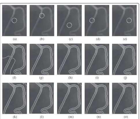
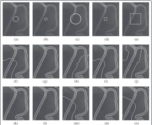
This can be seen from a simple experiment for an X-ray vessel image that used in [14]. Figure 1 shows the segmen-tation results of the RSF model for the vessel image with five different initial contour locations (circles with the same size but different positions). The initial contours over the original image are shown in the upper row of Figure 1. From the second row of Figure 1, we observe that the RSF model fails to extract the vessel for the first initial location (Figure 1(f)), although obtain satisfactory segmentation results for the other four locations (Figure 1(g)-(j)). Figure 2 displays the segmentation results of the RSF model for the vessel image with different initial contour sizes and shapes. The initial contours are chosen as circles and squares at the center of image but with different sizes, as shown in
the upper row of Figure 2. The segmentation results in the second row of Figure 2 show that the RSF model can only obtain accurate segmentation for the second initial contour (Figure 2(g)).
LIF model
For efficient segmentation, Zhang et al. [16] utilized the local image information and proposed a LIF energy functional by minimizing the difference between the fit-ted image and the original image. The formulation is expressed as:
ELIFð Þ ¼ϕ 1 2 Z
ΩjI xð Þ ðm1Hð Þ þϕ m2ð1Hð Þϕ ÞÞj 2
dx
ð11Þ
(a)
(b)
(c)
(d)
(e)
(k)
(l)
(m)
(n)
(o)
(f)
(g)
(h)
(i)
(j)
whereI(x) is the image to be segmented, whilem1and m2are two fitting functions defined as
m1¼meanðI2 ðx2Ω ϕj ð Þx <0g \WkðxÞÞÞ
m2¼meanðI2 ðfx2Ω ϕj ð Þx≥0g \WkðxÞÞÞ ð12Þ
Here, Wk(x) is a rectangular window, which is gener-ally chosen as a truncated Gaussian windowKσ (x) with standard deviationσand of size 4k× 4k(kis the greatest integer smaller thanσ).
Similar as the above three models, the LIF is also implemented by an alternative procedure: for each iter-ation and the corresponding level set function ϕn, we first compute the fitting valuesm1ð Þϕn andm2ð Þϕn , then obtain ϕnþ1 by minimizing ELIFð Þϕ with respect to ϕ.
This process is repeated until the zero-level set of ϕnþ1 is exactly on the object boundary.
The LIF model results in a local fitted image
ILFIð Þ ¼x m1Hðϕð Þx Þ þm2ð1Hðϕðð Þx ÞÞÞ: ð13Þ
It is also a PS approximation of the original image but with different fitting valuesm1andm2.
By using local region information, the LIF model is able to provide desirable segmentation results in the presence of intensity inhomogeneity. Although it is more efficient than the RSF model, it is still sensitive to contour initialization, like most existing localized active contours [14,16,25,26]. In practice, the LIF model initial contour has to carefully be selected for a satisfactory segmentation.
(a)
(b)
(c)
(d)
(e)
(k)
(l)
(m)
(n)
(o)
(f)
(g)
(h)
(i)
(j)
This can be seen from a similar experiment as the RSF model in Figures 1 and 2. Figure 1(k)-(o) shows the seg-mentation results of the LIF model for the vessel image with five distinct initial locations, which reveal that the LIF model extracts accurately the object only for the sec-ond and fourth initial contours (Figure 1 (l, n)). In Figure 2(k)-(o), we demonstrate the segmentation results of the LIF model for the vessel image with five initial contours of different sizes and shapes. From the results, we observe that the LIF model fails to segment the ves-sel image for the third and fifth initial contours (Figure 2 (m, o)), although it better captures the object for the other three initial contours (Figure 2 (k, l, n)).
The proposed model
The above-mentioned four models share the similar al-gorithm structure to find a PS (constant) approximation of the original image. The main difference is how to
define both the energy functional to be minimized and the PS function approximating the original image. In this section, pursuing the same idea we introduce different energy functional and PS function to search for the opti-mal PS approximation of the original image.
For a given image I:Ω⊂R2 !R and a level set func-tionψ, we first define two smooth functions as follows:
h1ðx;ψÞ ¼ Z
ΩZKσðxyÞIð Þy Hðψð Þy Þdy
ΩKσðxyÞHðψð Þy Þdy
; x2Ω
h2ðx;ψÞ ¼ Z
ΩZKσðxyÞIð Þy ð1Hðψð Þy ÞÞdy
ΩKσðxyÞð1Hðψð Þy ÞÞdy
ð14Þ
whereHis the Heaviside function, and Kσ is a Gaussian kernel function:
Kσð Þ ¼u 1 2π ð Þ1=2σe
j ju=2σ2
ð15Þ
with a scale parameter σ> 0. The functions h1ðx;ψÞand
h2ðx;ψÞare really the weighted averages of the image in-tensities in the regions fx:ψð Þx >0g and fx:ψð Þx ≤0g respectively, with KσðxyÞ as the weight assigned to the intensity I(y). The smoothness of h1ðx;ψÞ and
h2ðx;ψÞ can be confirmed by the Gaussian convolutions in (14).
Next, we introduce another level set function ϕ to al-ternate withψ, and finally find a level set functionϕ∗so that the following PS function:
IPS
ψ ðx;ϕ∗Þ ¼h1ðx;ψÞHðϕ∗ðxÞÞ þh2ðx;ψÞð1Hðϕ∗ðxÞÞÞ
¼ h1ðx;ψÞ; x 2fϕ∗>0g h2ðx;ψÞ; x 2 fϕ∗≤0g
ð16Þ
approximates optimally the original image I(x), in the sense of
EPSFψ ðϕ∗Þ ¼ min
ϕ E
PSF
ψ ð Þϕ ð17Þ
with
EPSFψ ð Þ ¼ϕ
Z
ΩjIð Þ x h1ðx;ψÞj 2
Hðϕð Þx Þdx
þ Z
ΩjIð Þ x h2ðx;ψÞj 2
1Hðϕð Þx Þ
ð Þdx
ð18Þ
where ϕ is a level set function over the image domain
Ω. The energy functional EPSF
ψ ð Þϕ can clearly be rewrit-ten as
EPSFψ ð Þ ¼ϕ
Z
Ω Ið Þ x I PS ψ ðx;ϕÞ
2dx ð19Þ
The energy functional EPSF
ψ ð Þϕ in (19) is in fact a square error of the approximation of the image I(x) by the PS function IPS
ψ ðx;ϕÞ; therefore, we call EψPSFð Þϕ the piecewise smooth fitting (PSF) energy.
As in typical level set methods [12,14,15,21], it is ne-cessary to smooth the zero-level set by penalizing its length:
Lð Þ ¼ϕ
Z
ΩjrHðϕð Þx Þjdx ð20Þ
In addition, for more accurate computation and stable level set evolution, we need to regularize the level set function by penalizing its deviation from a signed dis-tance function [13,28], which can be characterized by the following energy functional
Pð Þ ¼ϕ
Z
Ω 1
2ðjrϕð Þx j 1Þ 2
dx ð21Þ
The regularizing term Pð Þϕ intrinsically maintains the regularity of the level set function without the need for extra re-initialization procedures.
Therefore, the total energy functional of the proposed model is given by
EψðϕÞ ¼EPSFψ ðϕÞ þvLðϕÞ þμPðϕÞ
¼ Z
ΩjIh1j 2
Hð Þϕ dxþ
Z
ΩjIh2j 2
1Hð Þϕ
ð Þdx
þν
Z
ΩjrHð Þϕ jdxþμ Z
Ω 1
2ðjrϕj 1Þ 2
dx
ð22Þ
wherev,μ> 0 are constants to balance the terms. In practice, the Heaviside function H(z) needs to be approximated by a smooth functionHEð Þz , which is
typ-ically given by
HEð Þ ¼z 1
2 1þ
2 πarctan
z E
ð23Þ
Following the same algorithm structure as the four models mentioned in“Related studies” section, the pro-posed algorithm can simply be described as follows:
1. Initialize the level set functionψ0ð Þx , and setn= 0. 2. Compute the smooth functionsh1ðx;ψnÞand
h2ðx;ψnÞ.
3. Obtainϕnþ1ð Þx by minimizing the energy functional
Eψnð Þϕ .
(See figure on previous page.)
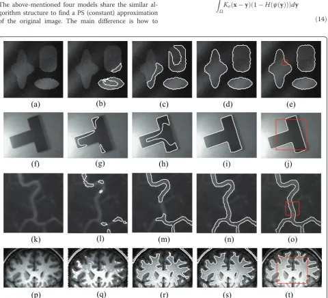
Figure 4Segmentations of four models for four real images with non-uniform backgrounds, starting with a constant functionψ0¼2.
(a)-(d): original images. (e)-(h): results of the Canny algorithm (left to right:σ¼1;T¼½0:02;0:2;σ¼1;T¼½0:2;0:3;σ¼2:2;T¼½0:09;0:7;σ¼ 2:2;T¼½0:09;0:4). (i)-(l): results of the CV model (5, 5, 300, 500 iterations). (m)-(p): results of the RSF model (left to right:ν¼0:01255255 with 300 iterations,ν¼0:008255255with 560 iterations,λ2¼1:2;ν¼0:008255255 with 300 iterations,ν¼0:004255255 with
4. If the zero-level set ofϕnþ1ð Þx is exactly on the
object boundary, then stop; otherwise, letn=n+ 1
andψnð Þ ¼x ϕnð Þx , then return to Step 2.
Note that the minimization problem in step 3 can be solved by the standard gradient descent method [29]. In detail, for ψn, we minimize Eψnð Þϕ with respect to ϕ by
solving the following gradient flow equation:
@ϕ
@t ¼ δEðϕÞ Ih1 x;ψ n
ð Þ
ð Þ2 Ih
2ðx;ψnÞ
ð Þ2
þνδEðϕÞdiv rϕ rϕ j j
þμ Δϕdiv rϕ rϕ j j
ð24Þ
with the initial condition ϕð0;xÞ ¼ψnð Þx and Neumann boundary condition. In Equation (24),δEð Þz is the deriva-tive of the functionHEð Þz :
δEð Þ ¼z H0Eð Þ ¼z π1E2þE
z2 ð25Þ
Remarks:
The CV PC model can be considered as an extreme
case of the proposed model forσ ! 1. This can be
seen from the fact that limσ!1hiðx;ψÞ ¼
ciði¼1;2Þ[14].
For the regularized Heaviside functionHE, the
functionsh1ðx;ψÞandh2ðx;ψÞin (14) are well
defined for anyψ. In applications, we suggest that
the functionψ be simply initialized to a constant
function:
ψ0ð Þ ¼x ρ; x2Ω ð26Þ
where ρis a constant. Such constant initialization com-pletely eliminates the need of initial contours. We do not need to consider the problems such as the determin-ation of where and how to define the initial contours.
Experimental results
Equation (24) is numerically implemented using a simple finite differencing (forward-time central-space finite dif-ference scheme). All the spatial partial derivatives@ϕ=@x and @ϕ=@yare approximated by the central difference, and the temporal partial derivative @ϕ=@tis discretized
as the forward difference. The approximation of Equa-tion (24) can simply be written as
ϕkþ1
i:j ¼ϕki:jþΔt:L ϕki:j ð27Þ
whereL ϕki:j is the approximation of the right-hand side of Equation (24) by the above spatial difference scheme.
We next present the experiments on both synthetic and real images with intensity inhomogeneity, noise and
complex background. The function ψ is simply
initia-lized to a constant function: ψ0¼2 . Unless otherwise specified, we use the following default setting of the
parameters which are determined by experiments: σ¼
18 , E¼1:0 , μ¼1 , ν¼0:001255255 , space step h¼1(implied pixel spacing) and time step Δt¼0:1. All experiments were run under Matlab R2007a on a PC with Dual 2.7 GHz processor.
Figure 3 shows the segmentation process of our model for four typical images with intensity inhomogeneity taken from [14]. The four images, which are plotted in Figure 3a,f,k,p, are a synthetic image (79 × 75) with Gaussian noise, a real image of a T-shaped object (127 × 90), an X-ray image of blood vessel (103 × 131), and a brain MR image (119 × 78). The contours (zero-level set) evolution processes are shown in second to forth columns. Although there are no initial contours for such non-zero constant function, we see from the second column that the contours emerge automatically after a few iterations. For the sake of clarity, we also list the segmentation results of the RSF model as well as ini-tial contours (in red) in the last column of Figure 3. It can be seen from Figure 3 that our model obtains the similar results with the classical RSF model on the seg-mentation of images with intensity inhomogeneity.
The second example (see Figures 4 and 5) shows that our model can work well for images with noise or non-uniform background and images with multiple objects of inhomogeneous intensities, starting with a constant func-tion. Meanwhile, to further demonstrate the advantages of our model, we give the segmentation results of one traditional method (Canny edge detector [7]) and two famous active contour models (the CV model [12] and the RSF model [14]) for comparison. Note that, for the Canny edge detector, we implement the fix threshold ver-sion and optimize the method with respect toσ(the scale
(See figure on previous page.)
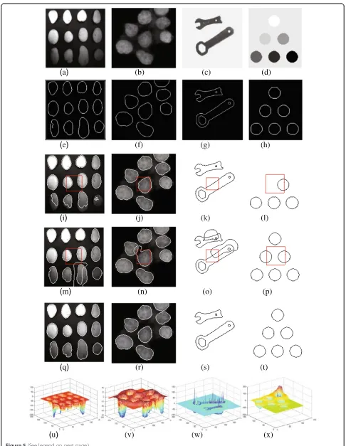
Figure 5Segmentations of four models for four images with multiple objects of inhomogeneous intensities or inside holes, starting with a constant functionψ0¼2.(a)-(d): original images. (e)-(h): results of the Canny algorithm (left to right:σ¼1;T¼½0:06;0:17;σ¼2;T¼
0:05;0:4
½ ;σ¼1;T¼½0:006;0:3;σ¼1;T¼½0:006;0:02). (i)-(l): results of the CV model (left to right:λ1¼3:5with 500 iterations,ν¼
0:015255255 with 500 iterations, 10, 300 iterations). (m)-(p): results of the RSF model (left to right:λ1¼1:2with 600 iterations,ν¼
0:01255255with 500 iterations, 500 iterations,λ1¼1:5;ν¼0:002255255 with 240 iterations). (q)-(t): results of our model (left to right:
parameter in the Gaussian filtering function Kσ) and to the gradient thresholds xT ¼ Tlow;Thigh
; for the CV and RSF models, the initial contours are necessary (we choose a square centered at the image with the size of 40 × 40 pixels for all the images in Figures 4, 5 and 6). Be-sides, we choose the best parameters for them (given in the Figure Caption) and list the best results we have obtained.
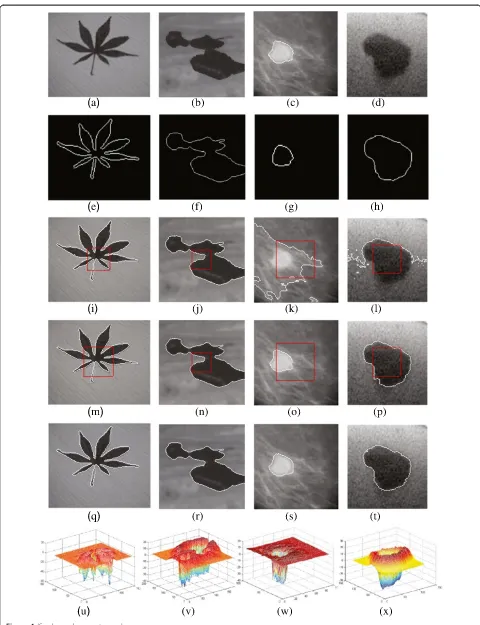
Figure 4 shows the segmentation results of four methods for four real images: a leaf image (122×120) with texture background, a chip image (182 × 180), a breast cyst image (91 × 92), and a CT medical image (117 × 123). Because of the influence of the texture, material properties, breast tis-sue, and the technical limitations, the backgrounds in these images are non-uniform, noise or even complex. Figure 4 (e)-(h) give the contours detected by Canny algorithm; we see that some contours detected by this algorithm are not continuous (Figure 4(e)). From the results of the CV model shown in Figure 4(i)-(l), we observe that, the CV model works well for images with less non-uniform (Figure 4(i) and (j)), however, if the level of non-uniform is higher, it fails to obtain exact segmentation results and identifies in-correctly some part of the background/foreground as the background/foreground (Figure 4(k) and (l)). Figure 4(m)-(p) shows the results of the RSF model; with fine-tuning parameters (given in the Figure Caption), the RSF model obtain satisfactory segmentation results expect for a little deficit in the lower left corner of the object in Figure 4(p). The results of our model and the corresponding 3D plots of final level set functions are shown in the last two rows of Figure 4. As can be seen from Figure 4(q)-(t), our model has effectively extracted object boundaries from the non-uniform and noisy background. For these four images, we chose large values forvto enhance the model’s robustness to noise:σ= 5 for Figure 4(a),σ¼20; ν¼0:003255 255 for Figure 4(b), ν¼0:0085255255 for Figure 4 (c) andσ¼12;ν¼0:003255255 for Figure 4(d).
Figure 5 show experiments on multiple objects and in-side holes segmentation. Figure 5(a)-(d) is: a potato image (157 × 157) with inhomogeneous intensities, a cell image (195 × 183) with one cell crossing the image boundary, a wrench image (200 × 200) with interior holes in each object, and a synthetic image (118 × 134) with seven different intensity values, respectively. Figure 5(e)-(h) give the contours detected by Canny algorithm; we see that it extracts the satisfactory object contours for
images with obvious intensity gradient (Figure 5(f )-(h)), but the contour detected for another image is disturbed by non-uniform intensity (Figure 5(e)). From the results of the CV model shown in Figure 5(i)-(l), we observe that, the CV model can deal with homogeneous images with multiple objects or inside holes (Figure 5(f ) and (g)), but if the intensity in such images are inhomogen-eous, it fails to obtain the whole boundaries for all of the objects (Figure 5(i) and (l)). Figure 5(m)-(p) shows the best segmentation results of the RSF model we obtained by tuning parameters; it obtain the exact result only for the last image (Figure 5(p)). The results of our model and the corresponding 3D plots of final level set func-tions are shown in the last two rows of Figure 5. As can be seen from Figure 5(q)-(t), our method detects all the objects, even though the object intensity is inhomogen-eous and some edges are blurry.
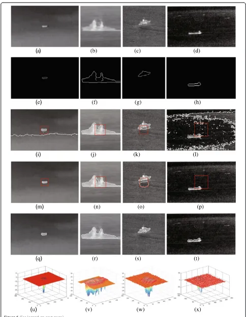
The third example presented in Figure 6 demonstrates that our model is especially suitable for segmentation of infrared ship images with low contrast, blurry edges and complex (noisy) background. Because of the limitation of thermal imaging and the actual water-mountain-sky conflicts, infrared images always suffers from low con-trast and complex background; thus, it is not a trivial task for most existing models to extract the objects (ships) in such images. As can be seen from Figure 6(e)-(h), Canny algorithm has difficulty dealing with such in-frared ship images, due to the presence of noise, low contrast, complex background and so on. To suppress noise effectively, a larger σ or a higher threshold T is needed, but a larger σ can result in edge shifting or in-accurate edge location (Figure 6(s)) and a higher T al-ways causes edge leaking (Figure 6(r)). From the results of the CV model shown in Figure 6(i)-(l), we observe that, the CV model obtain acceptable results in Figure 6 (j) and (k), but due to the intensity inhomogeneity and noise, it can’t obtain the exact object boundaries in Fig-ure 6(i) and (l). FigFig-ure 6(m)-(p) shows the segmentation results of the RSF model; it obtain the accurate results only for the first and the last image (Figure 6(m) and (p)). In contrast, our model, starting with a nonzero con-stant function, has successfully extracted the ships from the complex backgrounds, as shown in Figure 6(q)-(t). For noisy images, we increase the value of vto improve
the model’s performance: ν¼0:007255255 for
Figure 6(c) andν¼0:02255255 for Figure 6(d).
(See figure on previous page.)
Figure 6Segmentations of four models for four real infrared images with blurry edges and complex backgrounds, starting with a constant functionψ0¼2.(a)-(d): original images. (e)-(h): results of the Canny algorithm (left to right:σ¼1;T¼½0:01;0:3;σ¼1:3;T¼½0:03;0:4
;σ¼2;T¼½0:03;0:6;σ¼1:5;T¼½0:03;0:9). (i)-(l): results of the CV model (left to right: 500 iterations, 140 iterations,ν¼0:015255255 with 500 iterations,λ1¼1:2;ν¼0:02255255 with 500 iterations). (m)-(p): results of the RSF model (left to right: 40 iterations,λ1¼1:2;ν¼
0:005255255with 500 iterations,λ1¼1:2;ν¼0:007255255 with 1000 iterations,ν¼0:06255255 with 280 iterations). (q)-(t):
Conclusion
In this article, we propose a novel image segmentation algorithm by PS approximation. The proposed model, which pursues the basic ideas behind four well-known region-based models, introduces different energy func-tional and PS functions to find the optimal PS approxi-mation of the original image. The initial function can be chosen as a constant function, which completely elimi-nates the need of initial contours. The proposed model is very appropriate for a wider range of images, including images with intensity inhomogeneity and infrared images with low contrast and complex background.
Competing interests
The authors declare that they have no competing interests.
Acknowledgements
This work is supported by the National Natural Science Foundation of China under Grant No. 61202349 and No. 11201506.
Author details
1College of Mathematics, Chongqing Normal University, Chongqing 401331,
China.2College of Mathematics and Statistics, Chongqing University, Chongqing 401331, China.
Received: 24 October 2011 Accepted: 3 September 2012 Published: 24 September 2012
References
1. L He, Z Peng, B Everding, X Wang, CY Han, KL Weiss, WG Wee, A comparative study of deformable contour methods on medical image segmentation. Image Vision Comput.26(2), 141–163 (2008)
2. G Papari, N Petkov, Edge and line oriented contour detection: state of the art. Image Vision Comput.29, 79–103 (2011)
3. NR Pal, SK Pal, A review on image segmentation techniques. Pattern Recogn.26(9), 1277–1294 (1993)
4. S Wang, JM Siskind, Image segmentation with ratio cut. IEEE Trans. Pattern Anal. Mach. Intell.25(6), 675–690 (2003)
5. SK Nath, K Palaniappan, Fast graph partitioning active contours for image segmentation using histograms. EURASIP J. Image Vide.2009, 9 (2009) 6. S Chabrier, C Rosenberger, B Emile, H Laurent, Optimization-based image
segmentation by genetic algorithms. EURASIP J. Image Vide.2008, 1–10 (2008)
7. J Canny, A computational approach to edge detection. IEEE Trans. Pattern Analysis and Machine Intelligence8, 679–714 (1986)
8. R Kimmel, AM Bruckstein, On regularized Laplacian zero crossings and other optimal edge integrators. Int. J. Comput. Vis.53(3), 225–243 (2003) 9. L He, S Zheng, L Wang, Integrating local distribution information with level
set for boundary extraction. J. Vis. Commun. Image R.21, 343–354 (2010) 10. V Caselles, F Catte, T Coll, F Dibos, A geometric model for active contours in
image processing. Numer. Math.66, 1–31 (1993)
11. V Caselles, R Kimmel, G Sapiro, Geodesic active contours. Int. J. Comput. Vis.
22(1), 61–79 (1997)
12. TF Chan, LA Vese, Active contours without edges. IEEE Trans. Image Process.
10(2), 266–277 (2001)
13. C Li, C Xu, C Gui, MD Fox, inProceedings of IEEE conference on Computer Vision and Pattern Recognition (CVPR), ed. by, 1st edn. (San Diego, CA, USA, 2005), pp. 430–436
14. C Li, C Kao, JC Gore, Z Ding, Minimization of region-scalable fitting energy for image segmentation. IEEE Trans. Image Process.17(10), 1940–1949 (2008)
15. L Wang, C Li, Q Sun, D Xia, C Kao, Active contours driven by local and global intensity fitting energy with application to brain MR image segmentation. Comput. Med. Imaging Graph.33(7), 520–531 (2009) 16. K. Zhang, H. Song, L. Zhang, Active contours driven by local image fitting
energy. Pattern Recognit.43, 1199–1206 (2010)
17. Y Wang, C He, Adaptive level set evolution starting with a constant function. Appl. Math. Model.36, 3217–3228 (2012)
18. S Osher, JA Sethian, Fronts propagating with curvature-dependent speed: algorithms based on Hamilton-Jacobi formulations. J. Comput. Phys.79, 12–49 (1988)
19. D Mumford, J. Shah, Optimal approximation by piecewise smooth functions and associated variational problems. Commun. Pure Appl. Math.42(5), 577–685 (1989)
20. X Wang, L He, WG Wee, Deformable contour method: a constrained optimization approach. Int. J. Comput. Vis.59(1), 87–108 (2004)
21. LA Vese, TF Chan, A multiphase level set framework for image segmentation using the Mumford and Shah model. Int. J. Comput. Vis.50(3), 271–293 (2002) 22. A Tsai, A Yezzi, AS Willsky, Curve evolution implementation of the
Mumford–Shah functional for image segmentation, denoising, interpolation, and magnification. IEEE Trans. Image Process.10(8), 1169–1186 (2001) 23. S Lankton, A Tannenbaum, Localizing region-based active contours. IEEE
Trans. Image Process.17(11), 2029–2039 (2008)
24. T Brox, D Cremers, On the statistical interpretation of the piecewise smooth Mumford–Shah functional, inProceedings of the Scale Space Methods and Variational Methods (SSVM’07), vol. 4485 of Lecture Notes in Computer Science
(Ischia, Italy, 2007), pp. 203–213
25. J Piovano, M Rousson, T Papadopoulo, Efficient segmentation of piecewise smooth images, inProceedings of the Scale Space Methods and Variational Methods (SSVM’07)(Lecture Notes in Computer Science, Ischia, Italy, 2007), pp. 709–720
26. C Li, C Kao, J Gore, Z Ding, Implicit active contours driven by local binary fitting energy, inProceedings of IEEE conference on Computer Vision and Pattern Recognition (CVPR)(, Washington, USA, 2007), pp. 1–7 27. S Gao, TD Bui, Image segmentation and selective smoothing by using
Mumford–Shah model. IEEE Trans. Image Process.14(10), 1537–1549 (2005) 28. C Li, C Xu, C Gui, MD Fox, Distance regularized level set evolution and its
application to image segmentation. IEEE Trans. Image Process.19(12), 3243–3254 (2010)
29. G Aubert, P Kornprobst,Mathematical Problems in Image Processing: Partial Differential Equations and the Calculus of Variations, 2nd edn. (Springer, New York, 2002)
doi:10.1186/1687-5281-2012-16
Cite this article as:Wang and He:Image segmentation algorithm by piecewise smooth approximation.EURASIP Journal on Image and Video Processing20122012:16.
Submit your manuscript to a
journal and benefi t from:
7Convenient online submission
7Rigorous peer review
7Immediate publication on acceptance
7Open access: articles freely available online
7High visibility within the fi eld
7Retaining the copyright to your article