www.ocean-sci.net/6/3/2010/
© Author(s) 2010. This work is distributed under the Creative Commons Attribution 3.0 License.
Ocean Science
Density and Absolute Salinity of the Baltic Sea 2006–2009
R. Feistel1, S. Weinreben1, H. Wolf2, S. Seitz2, P. Spitzer2, B. Adel2, G. Nausch1, B. Schneider1, and D. G. Wright3
1Leibniz Institute for Baltic Sea Research, 18119 Warnem¨unde, Germany 2Physikalisch-Technische Bundesanstalt, 38116 Braunschweig, Germany 3Bedford Institute of Oceanography, Dartmouth, NS, Canada
Received: 3 August 2009 – Published in Ocean Sci. Discuss.: 19 August 2009
Revised: 10 December 2009 – Accepted: 17 December 2009 – Published: 18 January 2010
Abstract. The brackish water of the Baltic Sea is a mixture of ocean water from the Atlantic/North Sea with fresh wa-ter from various rivers draining a large area of lowlands and mountain ranges. The evaporation-precipitation balance re-sults in an additional but minor excess of fresh water. The rivers carry different loads of salts washed out of the ground, in particular calcium carbonate, which cause a composition anomaly of the salt dissolved in the Baltic Sea in comparison to Standard Seawater. Directly measured seawater density shows a related anomaly when compared to the density com-puted from the equation of state as a function of Practical Salinity, temperature and pressure.
Samples collected from different regions of the Baltic Sea during 2006–2009 were analysed for their density anomaly. The results obtained for the river load deviate significantly from similar measurements carried out forty years ago; the reasons for this decadal variability are not yet fully under-stood. An empirical formula is derived which estimates Ab-solute from Practical Salinity of Baltic Sea water, to be used in conjunction with the new Thermodynamic Equation of Seawater 2010 (TEOS-10), endorsed by IOC/UNESCO in June 2009 as the substitute for the 1980 International Equa-tion of State, EOS-80. Our routine measurements of the samples were accompanied by studies of additional selected properties which are reported here: conductivity, density, chloride, bromide and sulphate content, total CO2and
alka-linity.
Correspondence to: R. Feistel ([email protected])
1 Introduction
In June 2009, the International Thermodynamic Equation of Seawater 2010 (TEOS-10, IOC, 2010) was endorsed by the IOC1 on its 25th General Assembly in Paris; it will be adopted as a new world-wide standard for oceanography on the 1 January 2010. TEOS-10 takes Absolute Salinity, SA,
(the mass fraction of sea salt in seawater) as its input variable to represent the concentration of dissolved sea salt in seawa-ter. This choice contrasts with its predecessor, the Interna-tional Equation of State of Seawater 1980 (EOS-80) which is formulated in terms of Practical Salinity, SP, measured
on the Practical Salinity Scale of 1978 (PSS-78) and repre-senting a measure of the conductivity of a seawater sample. For the first time in the history of oceanographic standards since 1902, this conceptual transition encourages an explicit consideration of composition anomalies in the world ocean (McDougall et al., 2009) as well as in estuaries such as the Baltic Sea. In practice, this choice requires the development of conversion formulae from Practical Salinity, available for example from a CTD cast, to Absolute Salinity involving additional parameters such as estimates of the composition anomalies or the geographic position, the depth and, if the anomalies vary significantly on seasonal or climatological scales, the time.
For the Baltic Sea, such an algorithm was first published by Millero and Kremling (1976), derived from extensive measurements (Kremling, 1969, 1970, 1972). Since later studies revealed relevant systematic changes of the empiri-cal coefficients (Kremling and Wilhelm, 1997), the first and main aim of this paper is to propose an updated empirical formula for the computation of Absolute Salinity of Baltic seawater, based on samples taken between 2006 and 2009, for use in conjunction with TEOS-10, as recommended by the IOC with its recent Resolution XXV-7 (IOC, 2009).
1IOC: Intergovernmental Oceanographic Commission,
4 R. Feistel et al.: Density and Absolute Salinity The composition anomaly of the salt dissolved in the
Baltic Sea compared to the composition of Standard Seawa-ter (Millero et al., 2008) is mainly caused by dissolution of CaCO3in river water and the subsequent input of Ca2+and
alkalinity/total CO2 into the Baltic Sea by river discharge
(Rohde, 1966; Nehring and Rohde, 1967; Kremling, 1969, 1970, 1972; Millero and Kremling, 1976). The alkalinity ex-cess controls the pH of the Baltic Sea surface water which at the present atmospheric CO2partial pressure ranges between
7.8 and 8.2 (Nehring, 1980) and is similar to the pH of ocean water (Millero, 2007; Marion et al., 2009). Below the perma-nent pycnocline, the pH may decrease to 7.0–7.3 (Fonselius, 1967) due to the the accumulation of CO2 by the
mineral-ization of organic matter. The second aim of this paper is to estimate the salinity anomaly on the basis of the state of the Baltic Sea CO2 system characterized by the alkalinity and
total CO2concentrations. On climatological time scales the
alkalinity in the Baltic Sea may increase because the rising atmospheric CO2may enhance the weathering of CaCO3in
the catchment area. The increased alkalinity input may affect the salinity anomaly but also has consequences for the Baltic Sea acid/base system since it counteracts the pH decrease as-sociated with increasing atmospheric CO2.
An estimate of the CaCO3excess of the Baltic Sea
com-pared to standard seawater is required for chemical compo-sition models of seawater such as FREZCHEM (Feistel and Marion, 2007) which can be used to evaluate the calcium car-bonate supersaturation in relation to atmospheric CO2levels
and its potential consequences (Marion et al., 2009; Comeau et al., 2009; Veron et al., 2009). Since the density anomaly of the Baltic Sea is varying on climatological time scales, the third aim of this paper is to provide a more recent anchor point for this model in relation to the extended similar in-vestigation made forty years ago by Kremling (1969, 1970, 1972) and Millero and Kremling (1976).
The fourth aim of this paper is a conceptual one, related to the former ones. The different oceanographic salinity scales that are in use since 1902 are not metrologically traceable to SI units (Seitz et al., 2008). Both PSS-78 and the recent Reference-Composition Salinity Scale (Millero et al., 2008) are defined in terms of relative conductivity measurements with artefacts such as IAPSO2Standard Seawater (SSW) or a potassium chloride solution used as a reference. Reliance on such artificial references introduces the risk of unnoticed or falsly indicated property changes over time or between dif-ferent samples. It would therefore be preferable to establish traceability to the highly reliable and independently realis-able standards of the International System of Units (Jones, 2009). The SCOR3/IAPSO Working Group 127 (WG127) on the Thermodynamics and Equation of State of Seawater
2IAPSO: International Association for the Physical Sciences of
the Ocean, http://iapso.sweweb.net
3SCOR: Scientific Committee on Oceanic Research,
http://www.scor-int.org
is currently developing a new concept for the measurement of Absolute Salinity based on SI-traceable density determi-nations (Wolf, 2008). The Baltic Sea with its strong density anomaly and pronounced trends in its properties is a promi-nent example of the need for the development of this ap-proach and a useful testing ground for the new but yet imma-ture calibration technology. For this reason, we have carried out comparison measurements of conductivity and density in an SI-traceable way and we report the results in this pa-per. The presentation of results is accompanied by selected chemical composition data.
The true Absolute Salinity is defined in terms of the mass fraction of dissolved material in seawater (Millero et al., 2008). As discussed by Millero et al., the precise defini-tion requires the determinadefini-tion of equilibrium condidefini-tions at specified temperature and pressure and even with these addi-tional qualifiers some ambiguity remains. In practice, mea-suring the mass fraction of dissolved material in seawater is even more difficult than defining it and approximate ap-proaches must be used. It is the “Millero Rule” that says that the density of an aqueous solution is in good approxima-tion a funcapproxima-tion of the Absolute Salinity, independent of the particular composition of the given mass of dissolved matter (Millero, 1974; Millero et al., 1978, 2008, 2009). Under this approximation, Baltic seawater and Standard Seawater have the same Absolute Salinity if they have the same density at given temperature and pressure. Thus, we can measure the density of Baltic seawater, and use the TEOS-10 equation of state to compute the Absolute Salinity of Standard Seawater with this density. We then use Millero’s Rule and take this “density salinity” as an estimate for the mass of salt dissolved in the Baltic Sea sample. We note however that the true Ab-solute Salinity is defined as the mass ratio of dissolved ma-terial and that Millero’s Rule provides an approximation to this quantity. Unfortunately, for seawater that is not of Ref-erence Composition there is currently no method available to precisely measure the Absolute Salinity, but Millero’s Rule provides an approximation that allows the density to be re-covered to the measurement accuracy (due to the use of the “density salinity” to estimate Absolute Salinity) as well as a useful approximation for other thermodynamic quantities that can be determined from the TEOS-10 Gibbs function (IAPWS, 2008; IOC, 2010; Feistel et al., 2009; Wright et al., 2009).
2 Salinity of standard and baltic seawater based on previous measurements
andP =101325 Pa (Culkin and Smith, 1980; SeaBird, 1989) and fromC, the temperatureT and the pressureP, Practical SalinitySPis computed from the function (Perkin and Lewis,
1980)
SP=s (C,T ,P ). (1)
Over the range of concentrations where Practical Salinity is defined, it can be converted to Reference Salinity, SR, by
the factoruPS=(35.16504 g kg−1)/35 (Millero et al., 2008,
Feistel, 2008):
SR=SP·uPS. (2)
For Standard Seawater, SR is the most accurate estimate
currently available for the Absolute Salinity. Given SR,
the corresponding density estimate can be determined from the Gibbs function g (SR,T ,P )of seawater (Feistel, 2008;
IAPWS, 2008; IOC, 2010):
ρ= 1
gP(SR,T ,P )
(3) Here, the subscriptP denotes the partial derivative with re-spect to the pressure, andT andP are the temperature and pressure at which the density is required, e.g. at laboratory conditions. T andP will be omitted from the equations be-low for simplicity. In the case of Standard Seawater, (Eq. 3) provides our best estimate of the true density,ρSSW. In the case of Baltic seawater, (Eq. 3) yields an apparent density that is subject to significant error. The anomaly of the true Baltic seawater density relative to this rather uncertain esti-mate can be determined by measuring the true density,ρBSW, with a vibration densitometer (Kremling, 1971; Millero and Kremling, 1976). The Absolute Salinity,SABSW=SR+δSA,
of Baltic seawater can then be estimated by the “density salinity”, i.e., by computing the Absolute Salinity of Stan-dard Seawater giving the measured density of Baltic seawa-ter, from the formula (Millero et al., 2008),
ρBSW= 1
gP(SR+δSA)
≈1+β·δSA
gP(SR)
, (4)
i.e.,δSA= ρBSWgP−1/β. Here,β= −gSP/gP is the
ha-line contraction coefficient.
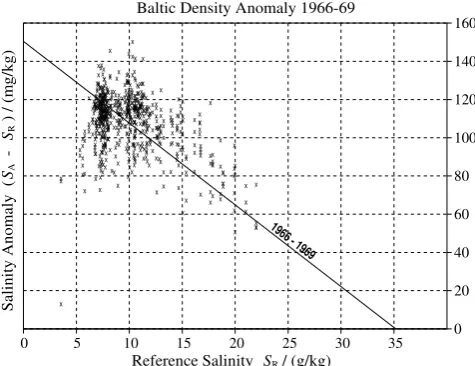
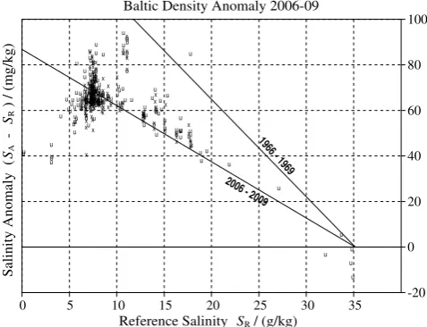
In Fig. 1, the anomalySABSW−SR is shown as a
func-tion ofSRfor 153 samples collected 40 years ago by
Krem-ling (1969, 1970, 1972), computed by means of (Eqs. 2–4) from the published values of measured Practical Salinity,SP,
and the measured density,
The correlation relating “density salinity” to Practical Salinity is easily obtained since both Practical Salinity and density are easily measured on a regular basis. Based on Kremling’s data, the regression line is
δSA=SA−SR=0.00428·(SSO−SR) =150mgkg−1·
1− SR
SSO
. (5)
0 5 10 15 20 25 30 35 0
20 40 60 80 100 120 140 160 Sa lin ity A no m al y ( SA - SR ) / ( m g/ kg )
Reference Salinity SR/ (g/kg)
Baltic Density Anomaly 1966-69
x x x x x x x x x x x x x xx x x x x x xx x xx x x x x x x x x x x x x x xx xx x x xx x x x x x x x x x x x x x x x x x x x x x x x xx x x x x x x x x x x x xx xx x x x x x x x x x x x x x x x x x x x x x x xx x x x xx x x x x x x x x x x x xx x x x x x x x x x xx xx xx x x x x xx x x x x x x x x x xx x x x xx x x x x x x x x x xx x x x x x x xx x xx x x x x x x x x x x x x x x x x x x x x x x x x x x x x x x x x x x x x x x xx xx x x xx x x x x x x x xx x x x x x x x xx x x x x x x x xxx x x x x x x x x x x x x x x x xx xx x x x x x xxx x x x x x x x x x x x xx x x xx x x x x x x x x x x x x x x x x x x x x x x x x x x x x x x x x x x x x x x x x x x xx xxx xx x xx x x x x x x x xx x x x x x x x x xx x xx x x x xx x x x x xx x x xxx x x x x x x x x x x x x xxx x x x x x x x x x x x x xx x x xx x x x x x x xx xx x x xxx x x x x xx x x x x x x x x x x x x xx x x x xx x xx x x x x x x x xxx x x x x x x x x xx x xx x x x xxx x x x x x x x x x x x x x xxx x x x xx x x x xx x x x x x x x x x x x x x x x x x x x x x xx x x x x x x x x x xxx x x xx x x xx x x xx x x x x x x xx x x xxx x xxx xx x x x xx x x x x x x x x x x xx x x x x x xxxxx
x x x xx xx x x x x x xx x x x xx x x x x x x x x x x x x xx x x x x x x x x x x x x x xx x x x x x xx x xxx xx x x x x x 1966
- 1969
Fig. 1: Salinity anomaly δSA=SA−SRcomputed by means of eqs. (2) - (4) from Practical
Salinity and density data measured by Kremling (1969, 1970, 1972) and Millero and Kremling (1976) in the period 1966-1969. The sample near SR = 4 g/kg with exceptionally
low anomaly was excluded from the fit (5); it was collected in the Vistula Estuary.
The strong scatter visible in Fig. 1 at very low salinities is due to the inhomogeneous water properties caused by the very different loads of the many discharging rivers. The sampling is patchy, but adequate for the present purpose. The calcium carbonate that is primarily responsible for the Absolute Salinity anomalies is mainly carried by rivers draining the European lowlands, while the Scandinavian rivers flow over solid rocks and are subsaturated with respect to lime (Kwiecinski, 1965). Spatial distributions of the river water age (Meier, 2007) indicate weak lateral mixing of the properties between the various rivers which contributes to the spatial inhomogeneity of the Baltic surface water. In lowest order, the structure of the mean surface current is evident from the climatological horizontal salinity gradient, Fig. 2 (Feistel et al., 2008). The Baltic has a mean basin-scale circulation that is predominantly estuarine (vertical) rather than horizontal (see the schematic flow diagram in Fig. 10.1 of Matthäus et al., 2008, available at
http://www2008.io-warnemuende.de/baltic2008/figures/figures_of_chapter_10.pdf ). Precipitation and fresh riverine water is added to the surface, and over time the surface water is enriched with salt from below by entrainment. The diffusive transport of saline water into the Baltic from the North Sea is negligible and strongly dominated by the permanent upward salt transport through the halocline at about 60 m depth, which has been roughly estimated as 30 kg m–2 yr–1, consistently from different approaches (Feistel et al., 2008; Reissmann et al.,
2009). Consequently, the climatological surface salinity increases following the mean surface flow from the north-east to the south-west. Brackish surface water is present in the outflow
Fig. 1. Salinity anomalyδSA=SA−SRcomputed by means of
(Eqs. 2–4) from Practical Salinity and density data measured by Kremling (1969, 1970, 1972) and Millero and Kremling (1976) in
the period 1966–1969. The sample nearSR=4 g/kg with
excep-tionally low anomaly was excluded from the fit (Eq. 5); it was col-lected in the Vistula Estuary.
The fit was constrained to pass through (SR=SSO, δSA=
0) because the Atlantic water part of the brackish mix-ture is free of the Baltic anomaly (Millero and Kremling, 1976). Here, the standard-ocean salinity isSSO=35uPS=
35.16504gkg−1(Millero et al., 2008).
6 R. Feistel et al.: Density and Absolute Salinity
branch of the Baltic “conveyor belt” that drives the Baltic Current along the Norwegian coast;
saltier water from the North Sea is flowing in at the bottom. In the shallow Belt Sea, strong
mixing occurs between the inflowing and outflowing layers that implies a recirculation of
significant freshwater fractions as a part of the salty bottom water.
In addition to the salt, entrainment from below the pycnocline adds aged, mixed and possibly
chemically transformed riverine solutes to the surface layer (Reissmann et al., 2009). In the
deep water of the estuarine Baltic Sea environment, the dissolved species may be subjected to
either reducing or oxidizing conditions that are sustained for extended periods of time
(Nausch et al., 2008). The time scales associated with these processes are of the order of
decades (Stigebrandt and Wulff, 1989; Meier et al., 2006; Feistel et al., 2008).
53°N 54°N 55°N 56°N 57°N 58°N 59°N 53°N 54°N 55°N 56°N 57°N 58°N 59°N 60°N 61°N 62°N 63°N 64°N 65°N 66°N 18°E 19°E 20°E 21°E 22°E 23°E 24°E 25°E 26°E 27°E 28°E 29°E
9°E 10°E 11°E 12°E 13°E 14°E 15°E 16°E 17°E 18°E 19°E 20°E 21°E 22°E 23°E 24°E 25°E 26°E 27°E 28°E 29°E BALTIC Climatological Dataset, 1° x 1°
Quantity: Salinity Unit: psu
Climatology: Annual, 1900- 2005
1. Cell Data: Cell Mean Value 2. Cell Data: Root Mean Square 3. Cell Data: Minimum Found 4. Cell Data: Maximum Found 5. Cell Data: Samples Count
Compiled by IOW on: 26.06.2007 14:31:05 Latitude Range [deg]: 53 to 65
Longitude Range [deg]: 9 to 29 Depth Range [m]: 0 to 10
Cell Invalid: blank
Cell Definition (lon): Integer Part Cell Definition (lat): Integer Part Cell Definition (depth): All Within Range Cell Definition (time): UTC Calendar Year, Month
20.74 3.29 4.02 32.62 440 28.65 3.42 12.41 34.57 2061 32.71 1.18 23.9 35.4 14152 18.98 2.63 10.37 31.6 28608 16.1 2.1 11.84 21.38 504 25.2 3.87 5.84 34.04 2356 29.44 3.03 10.16 35.13 8895 28.34 3.66 9.66 35.14 14781 23.18 3.32 10.44 33.35 25726 18.4 3.15 7.4 33.35 74991 15.89 2.8 5 29.5 30602 14.38 2.64 5.45 20.72 237 23.07 4.71 6.3 34.27 129 26.23 3.45 6.05 34.51 8915 24 3.65 6.4 34.61 21514 19.74 3.29 8.88 33.9 14449 15.48 3.46 6.31 34.1 20394 12.87 2.73 5.08 26.81 39742 12.38 1.55 10.1 17.57 141 20.59 3.05 9.74 33.8 962 18.13 3.5 5.2 34.4 26395 11.94 3.55 4.81 35.7 58315 10.49 1.89 5.08 25 141066 8.01 0.53 5.98 21.52 17417 8.02 0.55 1.87 17.12 70156 7.74 0.38 5.39 11.05 24862 7.67 0.52 2.65 10.62 28910 6.35 0.8 1.58 8.67 2454 7.57 0.29 6.6 9.14 600 7.56 0.3 3.4 9.5 36838 7.63 0.33 3.38 9.47 10651 6 0.67 3.08 7.29 22 7 0.38 4.78 7.85 355 7.29 0.34 5.1 8.64 1271 7.55 0.3 3.1 9.36 21552 7.48 0.3 5.46 8.98 1824 5.07 0.48 3.07 6.09 453 5.4 0.33 3.59 6.04 790 5.16 0.36 3.59 5.76 27 6.02 0.05 5.97 6.1 3 6.79 0.4 5.48 8.17 2016 6.99 0.32 5.69 8.94 5053 7.19 0.33 4.77 8.5 990 7.53 0.31 4.65 9.17 9849 7.36 0.26 6.62 8.09 423 4.94 0.57 2.03 5.88 273 5.2 0.38 2.94 6.14 1287 5.55 0.26 3.2 6.35 1483 5.6 0.31 3.62 6.49 1837 5.79 0.56 4.24 7.07 160 6.67 0.38 5.14 8.06 5569 7.06 0.33 5.92 8.66 731 7.32 0.47 5.27 10.85 8350 7.45 0.3 3.29 9.4 11346 7.1 0.59 1.04 8.29 3570 4.58 0.76 1.07 6.15 616 5.39 0.33 4.07 6.21 1857 5.71 0.22 3.39 6.17 1825 5.58 0.31 3.91 6.5 4369 5.97 0.37 4.8 7.46 3050 6.9 0.34 4.38 7.89 4116 7.23 0.32 3.3 8.37 12207 7.38 0.29 5.53 8.14 10335 7.48 0.28 3.49 8.73 3158 7.35 0.37 1 8.19 7087 4.77 0.59 1.08 6.91 3443 5.44 0.33 3.36 6.3 2398 5.75 0.22 3.01 6.41 3359 5.97 0.29 3.27 6.53 519 6.45 0.48 4.82 9.39 1237 6.83 0.38 4.42 8.02 3820 7.27 0.32 5.84 8.62 20675 7.17 0.29 3.92 8.17 2793 7.28 0.29 5.89 7.98 1457 6.64 0 6.64 6.64 2 3.11 0.48 2.43 3.46 6 3.22 0.25 2.13 3.9 633 3.96 0.42 1.96 5.5 3094 5.25 0.36 1 6.16 1120 5.6 0.3 1.26 6.43 3640 6.06 0.26 1.15 6.94 5881 6.61 0.39 3.12 7.81 5672 6.93 0.37 5.83 7.63 208 6.98 0.42 3.71 7.65 899 6.96 0.14 6.65 7.1 65 6.62 0.32 2.55 7.32 270 2.74 0.61 1 3.37 69 3.34 0.22 2.64 4.53 2029 3.42 0.24 1.02 5.14 2039 6.07 0.19 5.31 6.44 77 6.32 0.46 2.36 7.54 6067 5.69 0.11 5.52 5.86 27 5.48 0.34 4.6 6.93 405 3.06 0.37 1.33 3.92 855 3.36 0.19 1.04 5.14 3367 3.38 0.21 2.81 3.66 41 2.37 0.26 1.06 4.4 24 5.99 0.65 1 8.16 6184 5.32 0.46 3.4 6.85 230 5.27 0.31 1.39 7.36 1382 2.95 0.35 1 3.9 2528 3.47 0.22 3 4.03 131 5.45 0.51 1.53 6.5 1300 5.69 0.51 1.51 7.23 7465 4.8 0.58 2.4 5.73 350 5.02 0.44 1.21 5.76 680 2.35 0 2.3 2.39 2 5.31 0.49 1.06 6.93 2946 5.35 0.54 2.98 8.44 3174 4.75 0.52 1.31 7.15 2194 4.97 0.63 2.88 6.78 704 4.11 0.51 1 5.64 5193 4.47 0.5 1.4 5.88 478 2.87 0.67 1.02 5.7 1282 4.04 0.8 1.65 5.89 71 2.27 0.69 1 5.19 688 Mean r.m.s. Min Max Count
Salinity [psu] Annual
BALTIC - IOW 2007
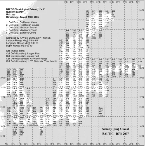
Fig. 2: Climatological surface distribution of Practical Salinity from the Baltic Atlas of
Long-Term Inventory and Climatology (BALTIC, Feistel et al., 2008). For each grid
cell of 1° x 1° x 10 m size, Practical Salinity values measured during 1900 – 2005 are
represented by the mean value, the root-mean square (r.m.s.) deviation, the minimum
Fig. 2. Climatological surface distribution of Practical Salinity from the Baltic Atlas of Long-Term Inventory and Climatology (BALTIC,Feistel et al., 2008). For each grid cell of 1◦×1◦×10 m size, Practical Salinity values measured during 1900–2005 are represented by the
different approaches (Feistel et al., 2008; Reissmann et al., 2009). Consequently, the climatological surface salinity in-creases following the mean surface flow from the north-east to the south-west. Brackish surface water is present in the outflow branch of the Baltic “conveyor belt” that drives the Baltic Current along the Norwegian coast; saltier water from the North Sea is flowing in at the bottom. In the shallow Belt Sea, strong mixing occurs between the inflowing and outflowing layers that implies a recirculation of significant freshwater fractions as a part of the salty bottom water.
In addition to the salt, entrainment from below the pycno-cline adds aged, mixed and possibly chemically transformed riverine solutes to the surface layer (Reissmann et al., 2009). In the deep water of the estuarine Baltic Sea environment, the dissolved species may be subjected to either reducing or ox-idizing conditions that are sustained for extended periods of time (Nausch et al., 2008). The time scales associated with these processes are of the order of decades (Stigebrandt and Wulff, 1989; Meier et al., 2006; Feistel et al., 2008).
In the special case in which the stoichiometric deviation from the Reference Composition is caused by an excess of non-conducting solutes with low concentrations, the value of SR represents the mass fraction of sea salt with Reference
Composition in the sample, andδSA represents the
anoma-lous mass fraction of non-conducting species, at least to a practically reasonable accuracy. This can safely be assumed for the silicate anomaly in the North Pacific (McDougall et al., 2009), but it is not generally the case in the Baltic Sea since the additional CaCO3 dissociates and increases
the conductivity by a non-zero amount, evidently less than what would result from adding the same mass of sea salt that has Reference Composition. Similarly, the algorithms used to estimate Practical Salinity at temperatures and pres-sures different from 15◦C and 101 325 Pa are not valid in the presence of the composition anomalies and (Eq. 1) results in inconsistent estimates, which can result in the appearance that the salinity is not conservative when subjected to tem-perature or pressure changes. Consequently, the correlation shown in Fig. 1 may look different depending on the particu-larT orP at which the measurements were carried out in the lab. However, a study dedicated to this problem (Feistel and Weinreben, 2008) came to the conclusion that these apparent non-conservation effects for Baltic seawater do not exceed the measurement uncertainty over a reasonable temperature interval at atmospheric pressure. Consequently, the param-eterisation of the Absolute Salinity of Baltic Sea water as a function of Reference Salinity is stable with respect to tem-perature variations at atmospheric pressure and is thus justi-fied for application in the context of TEOS-10 (IOC, 2010).
The above approach to estimating Absolute Salinity re-lies on an empirical relation between Absolute and Practical Salinity in the Baltic Sea. It does not permit the separate estimation of the contributions from riverine input into the Baltic Sea and from the sea salt flowing in from the Atlantic. This separation is possible using measurements of the
chlo-rinity, Cl, rather than conductivity since no relevant amounts of chlorine, bromine or iodine are discharged from the trib-utaries. Chlorinity can thus be used to estimate the Abso-lute Salinity contribution associated with input from the At-lantic and subtracting this value from the density salinity will provide an estimate of the contribution associated with local inputs. Millero and Kremling (1976) performed their corre-lation analysis based on chlorinity data. Two drawbacks of this method are that chlorinity is not a concentration measure to be used with TEOS-10, and silver titrations are not carried out regularly on modern research or monitoring cruises in the Baltic. Nevertheless, the approach can be used to separate the salt inputs from the Atlantic and from local runoff and to provide a comparison with the conditions found earlier by Knudsen (1901) and Sørensen (Forch et al., 1902).
For Standard Seawater, the Reference SalinitySRcan be
computed from the chlorinity by multiplying by the factor uCl=1.80655·uPS(Millero et al., 2008; Feistel, 2008). For
Baltic Sea water the result will differ fromSR, and is
there-fore referred to here as “chlorinity salinity”,SCl:
SCl=Cl·uCl=180655·Cl·uPS (6)
Using the chlorinity, Cl, and the density,ρBSW, data mea-sured by Kremling (1969, 1970, 1972) and Millero and Kremling (1976) together with (Eq. 4) in the form,
ρBSW= 1
gP SCl+δSRI
≈1+β·δS RI
gP(SCl)
, (7)
the regression line for the river input,δSRI, Fig. 3, is deter-mined as
δSRI=SA−SCl=000492·(SSO−SCl) =173mgkg−1·
1−SCl
SSO
. (8)
The difference between (Eqs. 5 and 8) is caused by the fact that the riverine input includes calcium carbonate and other solutes which alter the impact on the electrical conductivity compared to the effect of diluting with pure water whereas the riverine input includes no corresponding input of halides. Because of this latter fact, the intercept at SCl=0
corre-sponds to no contribution from North Atlantic water and pro-vides a direct estimate of the contribution to Absolute Salin-ity due to the salt content of the local riverine inputs.
Millero and Kremling (1976) did an analogous fit to their data set with 153 samples but found an intercept at zero chlo-rinity of onlySA0=124 mgkg−1. The reason for this differ-ence is probably the older equation of state used at that time (F. J. Millero, personal communication, 2009).
It is also possible to estimate the relation corresponding to (Eq. 8) based on data from the early 20th century. The Knudsen (1901) EquationSK=0.03gkg−1+1.805Cl, was
8 R. Feistel et al.: Density and Absolute Salinity
(
)
( )ClRI
RI Cl
BSW 1 1
S g
S S
S
gP P
δ β δ
ρ ≈ + ×
+
= , (7)
the regression line for the river input,δSRI, Fig. 3, is determined as
( − )= × − × = − = − SO Cl 1 Cl SO Cl A
RI 0.00492 173mgkg 1
S S S S S S S
δ . (8)
The difference between (5) and (8) is caused by the fact that the riverine input includes calcium carbonate and other solutes which alter the impact on the electrical conductivity compared to the effect of diluting with pure water whereas the riverine input includes no corresponding input of halides. Because of this latter fact, the intercept at SCl = 0 corresponds
to no contribution from North Atlantic water and provides a direct estimate of the contribution to Absolute Salinity due to the salt content of the local riverine inputs.
Millero and Kremling (1976) did an analogous fit to their data set with 153 samples but found an intercept at zero chlorinity of only 0 1
A=124mgkg−
S . The reason for this difference is probably the older equation of state used at that time (F.J. Millero, pers. comm.).
0 5 10 15 20 25 30 35 0
20 40 60 80 100 120 140 160 180 Sa lin ity A no m al y ( SA -
SCl
) /
(m
g/
kg
)
Chlorinity Salinity SCl/ (g/kg)
Baltic Density Anomaly 1966-69
x x x x x x x x x x x x x xx xx x x x xx x xxx x x x x x x x x x x x x xx xx x x xx x x x x x x x x x x x x x x x x x x x x x x x xx x x x x x x x x x x x xx xx x x x x x x x x x x x x x x x x x x x x x x xx x x x xxx x x x x x x x x x x xx x x x x x x x x x xx xx xx x x x x xx x x x x x x x x x xx x x x xx x x x x x x x x x xx x x xx x x x x x x x xx x xx x x x x x x x x x x x x x x x x x x x x x x x x x x x x x x x x x x x x x x xx xx x x xx x x xx x x xxx x x x x x x x xx x x x x x x x xxx x xx x x xx x x x x x x x x x x xx x x x x x xxx x x x x x xx x xxx xx x x xx x x x x x x x x x x x xx x x x x x x x x x x x x x x x x x x x x x x x x x x x x x xx xxx xx x xx x x x x x x x xx x x x x x x x x xx xxx x x x xx x x x x xx x x xxx x x x x x x x x x x x x xxx x x x x x x x x x x x x xx x x xx x x x x xx xx xx x x xxx x xx x xx x x x x x x x x x x x x xx x x x xx x x xx x x x x x x x xxx x x x x x x x x xx x xx x x x xxx x x x x x x x x xx x x x xxx x x x xx x x x xx x x x x x x x x x x x x x x x x xx x x x xx x xx x x x x x x xxx x x xx x x xx x x xx x x x x x x xx x x xxxxxxx xx x x x xx x x x x x x x x x x xx x x x x x x x xx x xx x xx xx x x x x x xx x x x xx x x x x x x x x x x x x xxx x x x x x x x x x x x x xx x x x x x xx x xxx xx x x x x x S S S S S S 1966
- 1969
Knudsen 1901
Fig. 3: Salinity anomaly associated with local runoff δSCl=SA−SClcomputed by means
of eqs. (4) - (6) from chlorinity and density data, symbol “x”, measured by Kremling (1969, 1970, 1972) and Millero and Kremling (1976) in the period 1966-1969. The sample with exceptionally low anomaly collected in the Vistula Estuary was excluded Fig. 3. Salinity anomaly associated with local runoffδSCl=SA−
SClcomputed by means of (Eqs. 4–6) from chlorinity and density
data, symbol “x”, measured by Kremling (1969, 1970, 1972) and Millero and Kremling (1976) in the period 1966–1969. The sam-ple with exceptionally low anomaly collected in the Vistula Estu-ary was excluded from the fit (Eq. 7) giving the line indicated by “1966–1969”. The “Knudsen 1901” (Eq. 9) was derived by Knud-sen (1901) from the measurements of SørenKnud-sen (Forch et al., 1902), Table 1, shown as symbol “S” in the diagram.
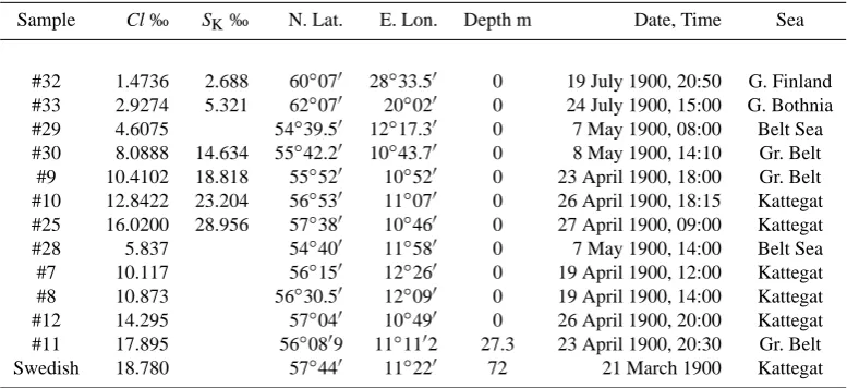
Great Belt and two from the Kattegat (Forch et al., 1902), which are reported for easy reference in Table 1.
The numerical value of SK in g/kg or ‰ coincides
with Practical Salinity (only) at SP=35 which was used
by PSS-78 to specify the coefficient relating SP to Cl.
Converting the chlorinity to a salinity estimate using (Eq. 6), SCl=Cl·uCl, effectively gives the Absolute Salinity of
Standard Seawater with this chlorinity. In addition, the absolute Knudsen salinity,SK, can be corrected for the loss
of volatile substances such as HCl using the factor relating Practical Salinity to Reference-Composition Salinity, thus providing an improved estimate of the true Absolute Salinity, SA=SK/ gkg−1·uPS. Using these two relations, the 1901
equation reads
SA−SCl=000086·(SSO−SCl)=30mgkg−1·
1−SCl
SSO
. (9) The uncertainties associated with this formula are unknown, but probably quite large due to the small number of data in-puts used to derive Knudsen’s formula. Nevertheless, the slope and the intercept corresponding to the Knudsen equa-tion are significantly lower than the more recent values, Fig. 3. Since the intercept atSCl=0 provides an estimate
of the “density salinity” of local riverine inputs, this seems to indicate that the calcium carbonate content of these inputs in-creased significantly between the end of the 19th century and 1970. In a similar regression, Ohlson and Anderson (1990)
0 5 10 15 20 25 30 35 40-50
-40 -30 -20 -10 0 10 20 30 40 50 Sa lin ity A no m al y ( SR -
SCl
) /
(m
g/
kg
)
Chlorinity Salinity SCl/ (g/kg)
Salinity-Chlorinity Anomaly 1966-69
x x x x x x x xx x x x x x x x x x x x x x x x x x x xx
x x x x x x x x x x x x x x x x x x x x x x x x x x x x x x x x x x x x x x x x x x x x x x x x x xxx x x x x x xx x x x x x x x x x x x x xxx
x x x x
x x x x x x x xx x x x x x x x x x x x
xxx x x x x
x x xx x x x x x x x x x x x x xx x x x xx x x x x x x x x x x x x x x x x x x x x x x x x x x x x x x x xx x x x x x x x x x x x x x x x x x x x x x x x x x x x x x x x x x x
1966 - 1969
Fig. 4: Deviation between the Reference Salinity (2), SR, and the chlorinity salinity (6),
SCl, computed from Kremling’s data collected between 1966 and 1969. Note that this
relation does not account for the additional contribution to Absolute Salinity given by (5) and illustrated in Fig. 1. The regression line (10) quantifies the average conductivity of the riverine water.
In a systematic study, Kwiecinski (1965) found that although the anomalous temporal or regional increase in the Practical Salinity usually follows that of calcium, there is no constant relation between them, and that additional factors such as the pH, the alkalinity or the dissolution of CO2 may be important. Numerical composition models (Anderko and Lencka,
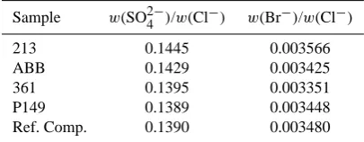
1997; Feistel and Marion, 2007; Pawlowicz, 2008, 2009) may provide more detailed insight in the future. The composition of the Baltic Sea salt measured by different authors was summarized by Nehring (1980) as given in Table 1 in comparison to the Reference Composition (Millero et al., 2008).
Table 1: Ratios rX = w(X)/Cl of mass fractions w(X) to chlorinity Cl of the main sea salt
constituents X compiled by Millero et al. (2008) for Standard Seawater and by Nehring (1980) for Baltic seawater from different sources. Molar masses AX are those compiled by
Millero et al. (2008). The oceanic value of rCl = [1/(0.3285234 AAg) – rBr/ ABr] ×ACl is
inferred from the definition of chlorinity, using the molar mass AAg = 107.8682(2) g/mol of
silver. The Baltic rCl is calculated from the same formula using Kremling’s value for rBr. The
numbers in brackets are the standard uncertainties of the corresponding digit(s) in front of the opening bracket.
Fig. 4. Deviation between the Reference Salinity (Eq. 2),SR, and
the chlorinity salinity (Eq. 6),SCl, computed from Kremling’s data
collected between 1966 and 1969. Note that this relation does not account for the additional contribution to Absolute Salinity given by (Eq. 5) and illustrated in Fig. 1. The regression line (Eq. 10) quantifies the average conductivity of the riverine water.
calculated the riverine calcium concentration rising from 521 µM (1938) to 571 µM (1967) and 878 µM (1986), which correspond to approximately 52, 57 and 88 mg/kg in terms of CaCO3, respectively. M used to be the unit of
amount-of-substance-concentration (molarity); its use is discouraged within the SI system. The results of Kremling and Wil-helm (1997) indicate that this increase continued between 1970 and 1995.
The relation between salinity, electrolytic conductivity and chlorinity in the Baltic Sea is not as well understood as for Standard Seawater (Millero et al., 2008). Krem-ling (1969, 1970, 1972) calculated separate correlation equa-tions between measured pairs of chlorinity and Practical Salinity values for different subsets of his data; the salin-ity intercepts at zero chlorinsalin-ity varied between 0.023 and 0.041. The difference between Reference Salinity (Eq. 2) and chlorinity salinity (Eq. 6) for Kremling’s data is displayed in Fig. 4 as a scatter plot. The regression line is given by,
SR−SCl=000058·(SSO−SCl)=20mgkg−1·
1−SCl
SSO
. (10) In the absence of ocean water,SCl=0, (Eq. 10) indicates a
residual Reference Salinity ofSR=20 mg/kg. Dividing by
uPSto convert to Practical Salinity and then using standard
algorithms to invert (Eq. 1) gives an average conductivity of aboutC≈2.7mSm−1for the Baltic river waters at 20◦C.
Table 1. Samples collected from the Baltic Sea in 1900 and analysed by Sørensen (Forch et al., 1902). It may be the extreme effort of salinity
determination by drying at 150–480◦C over 120 h that prevented Sørensen from the analysis of all available samples. Additional samples
taken from outside the Baltic Sea are omitted from this table.
Sample Cl ‰ SK‰ N. Lat. E. Lon. Depth m Date, Time Sea
#32 1.4736 2.688 60◦070 28◦33.50 0 19 July 1900, 20:50 G. Finland
#33 2.9274 5.321 62◦070 20◦020 0 24 July 1900, 15:00 G. Bothnia
#29 4.6075 54◦39.50 12◦17.30 0 7 May 1900, 08:00 Belt Sea
#30 8.0888 14.634 55◦42.20 10◦43.70 0 8 May 1900, 14:10 Gr. Belt
#9 10.4102 18.818 55◦520 10◦520 0 23 April 1900, 18:00 Gr. Belt
#10 12.8422 23.204 56◦530 11◦070 0 26 April 1900, 18:15 Kattegat
#25 16.0200 28.956 57◦380 10◦460 0 27 April 1900, 09:00 Kattegat
#28 5.837 54◦400 11◦580 0 7 May 1900, 14:00 Belt Sea
#7 10.117 56◦150 12◦260 0 19 April 1900, 12:00 Kattegat
#8 10.873 56◦30.50 12◦090 0 19 April 1900, 14:00 Kattegat
#12 14.295 57◦040 10◦490 0 26 April 1900, 20:00 Kattegat
#11 17.895 56◦0809 11◦1102 27.3 23 April 1900, 20:30 Gr. Belt
Swedish 18.780 57◦440 11◦220 72 21 March 1900 Kattegat
be important. Numerical composition models (Anderko and Lencka, 1997; Feistel and Marion, 2007; Pawlowicz, 2008, 2009) may provide more detailed insight in the future. The composition of the Baltic Sea salt measured by different au-thors was summarized by Nehring (1980) as given in Table 2 in comparison to the Reference Composition (Millero et al., 2008).
3 Experimental methods used for recent measurements
In this Sect. the experimental methods and uncertain-ties are described with regard to the samples col-lected from the Baltic Sea during the period 2006– 2009. Results of the measurements are reported in the digital Supplement (http://www.ocean-sci.net/6/3/2010/ os-6-3-2010-supplement.zip) of this paper.
3.1 Sample collection
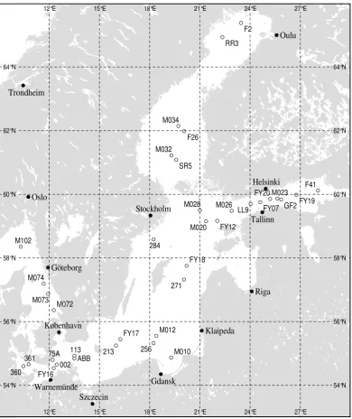
The Baltic Sea water samples were collected from 2006 to 2009 at the positions shown in Fig. 5. The bottle depth ranged between the surface and 400 m. A total of 438 sam-ples were analysed.
On the vessel, most of the samples were extracted into Duran-glass bottles (volume: 100 ml) by means of a CTD SBE-911 rosette equipped with IOW-freeflow samplers. Only the samples from the stations “FYxx” were collected from the cooling water inlet of the ferry and extracted into PET plastic bottles.
3.2 Routine salinometer and density measurements
For the determination of Practical Salinity, salinometers of the type AUTOSAL 8400B (Guildline Instruments, Canada) were used. Measurements of Practical Salinity were per-formed according to the rules of WOCE Operations and Methods (Stalcup, 1991). Once a day the salinometer was first adjusted with IAPSO Standard Seawater (SSW) and the SSW density was then determined with the densitometer.
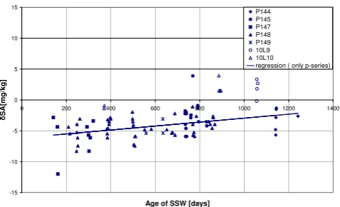
The results of the density measurements of Standard Sea-water are shown in Fig. 6. The deviations from zero must be attributed to the stability of the SSW samples and the measur-ing technique. The calculations refer to the Practical Salinity value given on the ampoule’s label. Practical Salinity mea-surements could not be done because the SSW samples were used for the calibration of the salinometer. For SSW (only P-series) we found a mean value of the difference δSA of −4.2 mg/kg with a standard deviation of 2.1 mg/kg. There is a slight dependence on the age of the sample. The related regression is line is
δSA/(mg/kg)=0.0032d−6.1453, (11)
wheredis the age of the samples in days. For SSW (10L-series) the distribution and number of measurements was in-adequate for reliable regression results to be obtained.
10 R. Feistel et al.: Density and Absolute Salinity
Table 2. RatiosrX=w(X)/Cl of mass fractionsw(X) to chlorinity Cl of the main sea salt constituents X compiled by Millero et al. (2008)
for Standard Seawater and by Nehring (1980) for Baltic seawater from different sources. Molar massesAXare those compiled by Millero et
al. (2008). The oceanic value ofrCl=[1/(0.3285234AAg)–rBr/ABr]·AClis inferred from the definition of chlorinity, using the molar mass
AAg=107.8682(2)g/mol of silver. The BalticrClis calculated from the same formula using Kremling’s value forrBr. The numbers in
brackets are the standard uncertainties of the corresponding digit (s) in front of the opening bracket.
Solute X
Molar Mass
g/molAX
Reference
Composition rX
Baltic Sea
rX
Baltic Sea Source
Na 22.989 769 28(2) 0.556 4924 0.5549–0.5562
0.5554 0.5547(21)
Zarins and Ozolins (1935) Culkin and Cox (1966) Kremling (1969)
K 39.0983(1) 0.020 6000 0.0200
0.0205 0.0206(6)
Zarins and Ozolins (1935) Culkin and Cox (1966) Kremling (1969)
Mg 24.3050(6) 0.066 2600 0.06692
0.0674(4) 0.067(3)
Voipio (1957)
Nehring and Rohde (1967) Kremling (1969, 1970, 1972)
Ca 40.078(4) 0.021 2700
Sr 8.762(1) 0.000 4100
Ca+Sr 0.021 6800 0.0225–0.0268
0.0218–0.0273
Rohde (1966)
Nehring and Rohde (1967) Kremling (1969, 1970, 1972)
Cl 35.453(2) 0.998 9041 0.998 9409
SO4 96.0626(50) 0.140 0000 0.1410
0.1413(19) 0.1436(42) 0.1406(10)
Zarins and Ozolins (1935) Kwiecinsky (1965) Trzosinska (1967)
Kremling (1969, 1970, 1972)
CO2 44.0095(9) 0.000 0220
Br 79.904(1) 0.003 4730 0.00329–0.00349
0.00339(6)
Morris and Riley (1966) Kremling (1969, 1970, 1972)
B 10.811(7) 0.00025(2) Kremling (1969, 1970, 1972)
B(OH)3 61.8330(70) 0.001 0030
B(OH)4 78.8404(70) 0.000 4100
F 18.998 4032(5) 0.000 0670 0.000078(4) Kremling (1969, 1970, 1972)
Because of the strong stratification in the Baltic Sea it must be assumed that the content of a 5 L-freeflow sampler is not necessarily homogeneous. For better results, 3 Duran bot-tles were filled. The measurements of salinity and density were done with seawater from the same glass bottle. Before the measurements were made, the bottle temperatures were adjusted to the room temperature (circa 23◦C). After uncap-ping the bottle a 20 ml disposable syringe was filled for the density measurements. Then the bottle was fitted with an adapter for a peristaltic pump. A peristaltic pump was con-nected to the salinometer for measuring the salinity of the sample.
High precision density measurements require very care-ful handling and elaborate procedures. To reduce the mea-surement uncertainty a procedure similar to that described by Wolf (2008) was used. Measurements were performed in the following order: with pure water (3 measurements), with the sample A (6 measurements), the sample B (6 measure-ments), and again with pure water (3 measurements). The formation of air bubbles inside the measuring cell was a se-vere problem that had to be solved. Baltic Sea water has typ-ical in-situ temperatures below the measuring temperature of the densitometer, 20◦C. Because of the reduced gas
Warnemünde Gdansk Szczecin
Klaipeda
Riga Tallinn
Helsinki
Stockholm
Göteborg
København Oslo
Oulu
Trondheim
002
113 213 256
271 284
360
361 ABB
GF2 F41
LL9 SR5
F2 RR3
F26
M020
M012
M010 M074
M102
M073 M072
M034
M032
M023 M026
M028 FY07
FY18
FY16
FY17
FY20
FY19
FY12
75A
54°N 56°N 58°N 60°N 62°N 64°N
54°N 56°N 58°N 60°N 62°N 64°N
12°E 15°E 18°E 21°E 24°E 27°E
12°E 15°E 18°E 21°E 24°E 27°E
Fig. 5: Positions where the recent samples used for this paper were collected. Stations “Mxxx” are from cruise AL322 of r/v “Alkor” in March 2009 and stations “FYxx”are from the ferry line “Finlandia” Travemünde - St. Petersburg in November 2008. “75A” was visited by r/v “Prof. A. Penck” on the research and monitoring cruise 40/06/20in August 2006, observing a baroclinic inflow (Matthäus et al., 2008). The remaining stations north of 59°N are from cruise Combine 1 of r/v “Aranda” in January 2009 and the remaining stations south of 59°N are from regular IOW monitoring cruises 2006-2008. Shorelines are from RANGS (Feistel, 1999).
Fig. 5. Positions where the recent samples used for this paper were collected. Stations “Mxxx” are from cruise AL322 of r/v “Alkor” in
March 2009 and stations “FYxx”are from the ferry line “Finlandia” Travem¨unde–St. Petersburg in November 2008. “75A” was visited by r/v “Prof. A. Penck” on the research and monitoring cruise 40/06/20 in August 2006, observing a baroclinic inflow (Matth¨aus et al., 2008).
The remaining stations north of 59◦N are from cruise Combine 1 of r/v “Aranda” in January 2009 and the remaining stations south of 59◦N
are from regular IOW monitoring cruises 2006–2008. Shorelines are from RANGS (Feistel, 1999).
which lead to significant errors in the readings. As a special procedure, the syringe to be filled was equipped with a hypo-dermic needle. After insertion into the sample the plunger of the syringe was pulled back rapidly. The limited filling rate through the narrow needle forced a low pressure in the sy-ringe and produced air bubbles in the sysy-ringe. These air bub-bles were pushed outside. Then the syringe was attached to the inlet of the densitometer and one half of the content was pushed into the measuring cell. Three measurements were
carried out and thereafter a further quarter of the syringe vol-ume was pressed inside and three additional measurements were done.
12 R. Feistel et al.: Density and Absolute Salinity 3.2Routine Salinometer and Density Measurements
For the determination of Practical Salinity, salinometers of the type AUTOSAL 8400B (Guildline Instruments, Canada) were used. Measurements of Practical Salinity were performed according to the rules of WOCE Operations and Methods (Stalcup 1991). Once a day the salinometer was first adjusted with IAPSO Standard Seawater (SSW) and the SSW density was then determined with the densitometer.
-15 -10 -5 0 5 10 15
0 200 400 600 800 1000 1200 1400
Age of SSW [days]
S
A
[m
g/
kg
]
P144 P145 P147 P148 P149 10L9 10L10
regression ( only p-series)
Fig. 6: Results of density measurements on standard seawater. Each data point represents a measurement of one bottle of SSW. P144 to P149 are batches of SSW with SP =35 and 10L9
and 10L10 are batches with SP = 10. On the ordinate, the apparent salinity anomaly is shown,
computed from (4), as a function of the sample age, in days.
The results of the density measurements of Standard Seawater are shown in Fig. 6. The deviations from zero must be attributed to the stability of the SSW samples and the measuring technique. The calculations refer to the Practical Salinity value given on the ampoule’s label. Practical Salinity measurements could not be done because the SSW samples were used for the calibration of the salinometer. For SSW (only P-series) we found a mean value of the difference SA of –4.2 mg/kg with a standard deviation of 2.1 mg/kg. There is a slight
dependence on the age of the sample. The related regression is line is
SA /(mg/kg) = 0.0032 d – 6.1453, (11)
where d is the age of the samples in days. For SSW (10L-series) the distribution and number of measurements was inadequate for reliable regression results to be obtained.
Measurements of the density were done by means of a densitometer DMA 5000 (Anton Paar, Austria). The device was calibrated daily with air and pure water. Measurements of the density and salinity were carried out at the same time as soon as possible after collecting the
Fig. 6. Results of density measurements on standard seawater. Each
data point represents a measurement of one bottle of SSW. P144
to P149 are batches of SSW withSP=35 and 10L9 and 10L10
are batches withSP=10. On the ordinate, the apparent salinity
anomaly is shown, computed from (4), as a function of the sample age, in days.
-50 0 50 100 150 200
0 10 20 30 40 50 60 70 80 90 100
Sample No
D
iff
er
en
ce
(n
ot
fi
lte
re
d
- f
ilt
er
ed
)
SA[mg/kg]
SR[mg/kg]
Fig: 7: Results of the comparison between filtered and unfiltered samples from the Baltic Sea. The particular pairs of samples were collected from the same CTD bottle but filled into separate flasks, subsequently. The symbols used together with the units are shown in the inset.
3.3“Absolute” Conductivity
Although the concept of an “absolute” measurement makes no sense from a strict metrological point of view, we will use this term for convenience to distinguish the measurements discussed here from those described in the previous section. Every quantity value that is indicated by a measuring device is inherently relative, since it is inevitably referred to something. Therefore metrological terminology prefers talking about traceability of a measurement result (VIM, 2008). This concept characterises the quantitative link between the indicated result and the quantity value that has been assigned to an agreed standard by a measurement or production procedure. The link is established by calibration measurements. In this sense the commonly measured conductivity ratio used to calculate practical salinity is traceable to the K15 ratio, which is indicated on Standard Seawater (SSW)
ampoules used for device calibration. K15 is the ratio of the electrical conductivity of the
seawater sample, at a temperature (IPTS-68) of 15 °C and a pressure of 101325 Pa, to that of a potassium chloride (KCl) solution, in which the mass fraction of KCl is 32.4356 g/kg at the same temperature and pressure. The production procedure for SSW according to PSS-78, which in particular links the electrolytic conductivity of SSW to that of the defined potassium chloride solution, must be seen as the corresponding primary procedure to realize K15. In
contrast, an “absolute” conductivity measurement result must be understood as traceable to the quantity value of a primary standard of the International System of Units (SI), which is realized by a primary measurement procedure. In the following we will use the expression “absolute” as a shorthand expression for this important concept of traceability.
Fig. 7. Results of the comparison between filtered and unfiltered
samples from the Baltic Sea. The particular pairs of samples were collected from the same CTD bottle but filled into separate flasks, subsequently. The symbols used together with the units are shown in the inset.
flasks were collected from the same water bottle of the CTD rosette. But this does not automatically imply that the water of both flasks has the same properties because the water in the bottle is usually stratified. Thus the shown difference of δSAbetween unfiltered and filtered samples depends not only
on the influence of filtration but also on the slightly different intrinsic properties of the two samples. We found a mean value of the difference ofδSA of 1.4 mg/kg with a standard
deviation of 4.9 mg/kg. For comparison, the differences of SRare additionally displayed in Fig. 7. The mean value of
the differences ofSRis 1.7 mg/kg with a standard deviation
of 20.4 mg/kg.
3.3 “Absolute” conductivity
Although the concept of an “absolute” measurement makes no sense from a strict metrological point of view, we will use this term for convenience to distinguish the measurements discussed here from those described in the previous section. Every quantity value that is indicated by a measuring de-vice is inherently relative, since it is inevitably referred to something. Therefore metrological terminology prefers talk-ing about traceability of a measurement result (VIM, 2008). This concept characterises the quantitative link between the indicated result and the quantity value that has been assigned to an agreed standard by a measurement or production pro-cedure. The link is established by calibration measurements. In this sense the commonly measured conductivity ratio used to calculate Practical Salinity is traceable to theK15 ratio,
which is indicated on Standard Seawater (SSW) ampoules used for device calibration. K15 is the ratio of the
electri-cal conductivity of the seawater sample, at a temperature (IPTS-68) of 15◦C and a pressure of 101 325 Pa, to that of
a potassium chloride (KCl) solution, in which the mass frac-tion of KCl is 32.4356 g/kg at the same temperature and pres-sure. The production procedure for SSW according to PSS-78, which in particular links the electrolytic conductivity of SSW to that of the defined potassium chloride solution, must be seen as the corresponding primary procedure to realize K15. In contrast, an “absolute” conductivity measurement
result must be understood as traceable to the quantity value of a primary standard of the International System of Units (SI), which is realized by a primary measurement procedure. In the following we will use the expression “absolute” as a shorthand expression for this important concept of traceabil-ity.
A measuring system for absolute electrolytic conductivity C calculates it from a conductance measurement of a con-ductivity measuring cell that is filled with the solution under investigation:
C=K·G. (12)
Kis the so called cell constant (not to be confused with the conductivity ratio K15 of SSW). Commercial conductivity
during the measurement is also measured and the measured conductivity value is corrected toT0.
In the present study we used the primary measurement method of the Physikalisch-Technische Bundesanstalt (PTB) (Brinkmann et al, 2003) to measure the absolute conductiv-ityCS of three samples from stations 361, ABB and 213,
Fig. 5. After arrival, the samples were stored under cold and dark conditions. Prior to measurement the samples and the conductivity measuring cell were brought to a set tempera-ture of 15◦C (ITS-90) over night in a temperature bath. We additionally measured the absolute conductivities CSSW of
IAPSO SSW/P-series (batch P149) and 10L10-series (Prac-tical Salinity 9.926, dated 14 June 2006) and calculated the conductivity ratio
R15=
CS
CSSW
K15 (13)
of the samples under investigation in order to scale the abso-lute conductivity measurement results to PSS-78.K15ratios
were taken from the SSW ampoules (0.99984 for P-series and 0.31712 for L10-series). Conductivity values have been linearly corrected to 15◦C (IPTS-68) using a temperature co-efficient of 1.97%/K. Finally we calculated Practical Salinity from the PSS-78 formula (Perkin and Lewis, 1980). The un-certainty of the absolute conductivity results includes contri-butions from the determination of temperature, conductance and the cell constant, and accounts for the statistical spread of the indicated values. Uncertainty propagation was calcu-lated according to GUM (2008).
3.4 High-accuracy density measurements
Highly accurate density measurements at the PTB Braun-schweig were performed for comparison with an oscillation-type density meter (Anton Paar DMA 5000) using a substi-tution method (Wolf, 2008). In a substisubsti-tution method the sample to be measured and a reference sample are measured alternately several times. This method decreases the mea-surement uncertainty considerably as contributions to the un-certainty are mostly correlated and thus vanish when looking for the difference between sample and reference.
The reference liquid was ultra pure degassed water. The deviation of its density from seawater is below 3%; thus, a very good correlation of the measurements performed on seawater and on ultra pure water is obtained provided that the handling of the samples is the same. The water we used was de-ionised reverse osmosis water Q water (Milli-pore, USA)) with a resistance of 18.2 Mcm and total or-ganic carbon of less than 10×10−9immediately after purifi-cation. It was made from Braunschweig tap water. The ref-erence density value was taken from the IAPWS-95 formu-lation (Wagner and Pruß, 2002). A correction was made for the isotopic composition. This was measured to be−8.5δ‰ for 18O and −59δ‰ for D compared to Vienna Standard
Mean Ocean Water. Thus, the density reference value for this Braunschweig tap water is 999.0996 kg/m3at 15◦C.
An uncorrelated uncertainty contribution is given by the reproducibility of the device measurement temperature 1treproducibility; it was measured to be below 3 mK. Another
uncertainty contribution arises from the deviation of the de-vice measurement temperature 1tdevice from the absolute
temperature. This can be expressed as a calibration uncer-tainty of the measurement temperature. With our device
1tdevice was measured to be 0 mK at 15◦C and −5 mK at
25◦C. The uncertainty of individual temperature measure-ments is±5 mK. Typical temperature deviations for other devices of the same type are 20 mK. The two temperature deviations act in a different way for seawater and for ultra pure water, as their effect on density is given by multiplying with the thermal expansion coefficientγ which is different for seawater and for ultra pure water:
ρpure water measured=
ρpure water(1+γpure water measured(1tdevice+1treproducibility))
ρseawater measured=
ρseawater(1+γseawater measured(1tdevice+1treproducibility)).
Here,ρpure water measuredandρseawater measuredare the densities
indicated by the measuring device, whereasρpure water and
ρseawaterdenote the real densities.
A third uncorrelated uncertainty contribution is caused by the different handling of the samples concerning its gas con-tent. The ultra pure water is degassed and will remain de-gassed during the measurement, whereas the seawater is sat-urated with air. The gas content is determined by the storage temperature of the seawater; during the short time the sam-ple is cooled or heated to the measuring temperature (about 15 min) no new equilibration will occur. Thus, the storage temperature affects the density by the gas content. This ef-fect can be reduced by storing the samples at well controlled reproducible conditions. In our measurements we stored the samples at refrigerator temperatures and warmed them up to room temperature over night before measuring. The contri-bution of this handling to the combined uncertainty (GUM, 2008) is not investigated up to now and, thus, estimated to be rectangular with a halfwidth of 0.5 ppm.
3.5 Ion chromatography
14 R. Feistel et al.: Density and Absolute Salinity The ion chromatography system used here consisted of a
Metrohm 881 Compact IC pro (Metrohm, Switzerland) with a Metrosep A Supp 5 column. The eluent was 3.2 mmol/L sodium carbonate plus 1 mmol/L sodium hydrogen carbon-ate.
All solutions were prepared gravimetrically using Milli-Q water (Millipore, USA). All seawater samples were diluted prior to injection. The calibration solutions were prepared from certified standard solutions delivered by Fluka (Fluka, Switzerland). The mass fractions as specified by the manu-facturer are for:
chloride:wCl=1003±3 mg/kg
sulphate:wSO4=1006±8 mg/kg
bromide:wBr=1003±4 mg/kg.
Calibration solutions containing similar mass fractions of an-ions as the seawater samples were prepared from the stan-dards. Three series of measurements, each using freshly pre-pared sample dilutions were generated for chloride, sulphate and bromide, respectively. Mean values of the mass frac-tions are reported from these measurements in Table 6. The relative expanded uncertainties (coverage factork=2) are 0.5% for chloride, 0.8% for sulphate and 1% for bromide. The main contributions to the measurement uncertainty are from the mass fractions of the certified standard solutions and from the preparation of the sample and calibration solution, respectively, by dilution.
4 Results
4.1 Parameterisation of Absolute Salinity
The 438 samples collected in the period 2006–2009 in the Baltic Sea between the Kattegat and the Gulf of Bothnia (Fig. 5) were analysed for Practical Salinity, Sect. 3.2, and density, Sect. 3.4. The related regression line computed from (4) using 436 samples with salinitySR>2 g kg−1is
SA−SR=0.00247·(SSO−SR) =86.9mgkg−1·
1− SR
SSO
, (14)
as shown in Fig. 8. Here, the standard-ocean salinity is SSO=35uPS=35.16504gkg−1(Millero et al., 2008).
Com-parison of (Eq. 3) with (5) suggests that the density anomaly has decreased by about 40% during the last 40 years. This result is in contrast to the findings of Dyrssen (1993), and of Kremling and Wilhelm (1997) that the mean calcium concentrations increased significantly by about 4% between 1966/69 and 1994/95.
The causes of the strong decadal variability are not known; it may be related to technical, agricultural or climatological changes in the drainage region of the Baltic Sea, and/or to the dramatic transition in the inflow regime from the North Sea
0 5 10 15 20 25 30 35 -20
0 20 40 60 80 100 Sa lin ity A no m al y ( SA - SR ) / ( m g/ kg )
Reference Salinity SR/ (g/kg)
Baltic Density Anomaly 2006-09
196 6 - 1969
u u u x x x uuu u u u x xx x x x u uu uu uuuuuuuxxxxxxuuu uuuuuuuu u u u u u u u u u uuu u u u x x x x x x x x x x x x xx x x xx x u u u u xx x x x u u u u uuuu xxx x xxxx u uuuu u u x u x u x u x u x u x uxu x u x u x ux u x u x u x u x u x u x u x u x uxu x u x u x ux u x u x u x u xux ux u u uu uuu u uu uuu u uu u u u u u u uuu uuu uuuuuuuu u uu uu uuuu u u uuu
u uu uuuu
uu x x u x u x x x u x ux x x ux u x x x ux ux x x u x ux xx uxux xx u x u x xx u
x x ux u x x x ux u x x x uxux x x ux ux x x ux u x x x uxx ux x ux x ux x u x u u xx u x x u x x ux x u x x uxx uxx u xx uxx u u u u uu u u u ux uuxu
x xx u u x u x u u x u ux uu x u u x uu x u u u
u u u u u uu u u u u u u u u u u u u u u u u u u u u u u u u u u u u u u uu u u u uuuu u
2006 - 2009
Fig. 8: The results of densitometer measurements in the Baltic Sea during 2006-2009, Fig. 5, converted to Absolute Salinity anomalies using eq. (4). Symbol “x”: filtered samples, “u”: unfiltered samples. 436 samples with salinity > 2 g kg –1 were used for the fit (14). At
vanishing Reference Salinity SR, the limiting anomaly isSA0=86.8mgkg−1. There is no
significant systematic difference between the fits using the data from filtered or unfiltered samples; the intercept is 87.0 mg/kg for only the 168 filtered “x” samples, and 86.6 mg/kg for only the 270 unfiltered “u” samples. The line marked 1966-1969 is the regression line (5) with regard to the data from 1966-69 of Millero and Kremling (1976), Fig. 1.
For three selected Baltic Sea water samples taken in November 2008 from the surface water at the stations 361 (Kiel Bight), ABB (Arkona Basin) and 213 (Bornholm Deep), Fig. 5, the analysis was repeated with state-of-the-art measurements of the absolute conductivity, section 3.3, and of density, section 3.5.
Table 2: Independent PTB measurements of conductivity and density of Baltic surface water at the selected stations 361, ABB and 213, Fig. 5, compared with the IOW data for density and Practical Salinity. All values are given at 15 °C and atmospheric pressure, except IOW density which was measured at 20 °C. Values for SA were computed from the related density
by means of (3). Note that the effect of temperature on density is automatically removed when calculating the “density salinity”, which is reported as SA. Related expanded uncertainties
(coverage factor 2) are given below the values
Fig. 8. The results of densitometer measurements in the Baltic Sea
during 2006–2009, Fig. 5, converted to Absolute Salinity anoma-lies using (Eq. 4). Symbol “x”: filtered samples, “u”: unfiltered
samples. 436 samples with salinity>2 g kg−1were used for the fit
(Eq. 3). At vanishing Reference SalinitySR, the limiting anomaly
isS0A=86.8mgkg−1. There is no significant systematic difference
between the fits using the data from filtered or unfiltered samples; the intercept is 87.0 mg/kg for only the 168 filtered “x” samples, and 86.6 mg/kg for only the 270 unfiltered “u” samples. The line marked 1966–1969 is the regression line (5) with regard to the data from 1966–69 of Millero and Kremling (1976), Fig. 1.
that occurred in the 1980s (Matth¨aus et al., 2008), and the related consequences for the marine chemistry in the deep water (Nausch et al., 2008).
For three selected Baltic Sea water samples taken in November 2008 from the surface water at the stations 361 (Kiel Bight), ABB (Arkona Basin) and 213 (Bornholm Deep), Fig. 5, the analysis was repeated with state-of-the-art measurements of the absolute conductivity, Sect. 3.3, and of density, Sect. 3.5.
The results, Table 3, of the comparison between mea-surements of density and conductivity at PTB and IOW can be pairwise combined to compute the salinity anomaly as a function of the Reference Salinity, Fig. 9. The four combina-tions are very close to each other and confirm the regression (Eq. 3) based on the full set of IOW measurements.