www.atmos-meas-tech.net/9/63/2016/ doi:10.5194/amt-9-63-2016
© Author(s) 2016. CC Attribution 3.0 License.
The development and evaluation of airborne in situ N
2
O and CH
4
sampling using a quantum cascade laser absorption
spectrometer (QCLAS)
J. R. Pitt1, M. Le Breton1, G. Allen1, C. J. Percival1, M. W. Gallagher1, S. J.-B. Bauguitte2, S. J. O’Shea1, J. B. A. Muller1,a, M. S. Zahniser3, J. Pyle4, and P. I. Palmer5
1School of Earth, Atmospheric and Environmental Sciences, University of Manchester, Oxford Road,
Manchester, M13 9PL, UK
2Facility for Airborne Atmospheric Measurements (FAAM), Building 125, Cranfield University, Cranfield,
Bedford, MK43 0AL, UK
3Aerodyne Research, Inc., Center for Atmospheric and Environmental Chemistry, Billerica, Massachusetts, USA 4Centre for Atmospheric Science, University of Cambridge, Cambridge, CB2 1EW, UK
5School of GeoSciences, University of Edinburgh, Edinburgh, EH9 3JN, UK
anow at: Deutscher Wetterdienst, Meteorologisches Observatorium Hohenpeißenberg, Hohenpeißenberg, Germany Correspondence to: J. R. Pitt ([email protected])
Received: 30 June 2015 – Published in Atmos. Meas. Tech. Discuss.: 27 August 2015 Revised: 30 November 2015 – Accepted: 3 December 2015 – Published: 15 January 2016
Abstract. Spectroscopic measurements of atmospheric N2O
and CH4 mole fractions were made on board the FAAM
(Facility for Airborne Atmospheric Measurements) large atmospheric research aircraft. We present details of the mid-infrared quantum cascade laser absorption spectrometer (QCLAS, Aerodyne Research Inc., USA) employed, includ-ing its configuration for airborne samplinclud-ing, and evaluate its performance over 17 flights conducted during summer 2014. Two different methods of correcting for the influence of wa-ter vapour on the spectroscopic retrievals are compared and evaluated. A new in-flight calibration procedure to account for the observed sensitivity of the instrument to ambient pres-sure changes is described, and its impact on instrument per-formance is assessed. Test flight data linking this sensitivity to changes in cabin pressure are presented. Total 1σ uncer-tainties of 2.47 ppb for CH4 and 0.54 ppb for N2O are
de-rived. We report a mean difference in 1 Hz CH4mole fraction
of 2.05 ppb (1σ=5.85 ppb) between in-flight measurements made using the QCLAS and simultaneous measurements us-ing a previously characterised Fast Greenhouse Gas Analyser (FGGA, Los Gatos Research, USA). Finally, a potential case study for the estimation of a regional N2O flux using a mass
balance technique is identified, and the method for calculat-ing such an estimate is outlined.
1 Introduction
CH4 and N2O emissions together comprise 38 % of the
to-tal global radiative forcing attributable to emissions of well-mixed greenhouse gases (Myhre et al., 2013). N2O is also a
major component of stratospheric chemical cycles, acting as the largest contributing species towards stratospheric ozone depletion, and predicted to remain so throughout the 21st century (Ravishankara et al., 2007). CH4emissions can also
lead to the formation of tropospheric ozone through reaction with OH radicals, leading to air quality issues associated with potentially dangerous respiratory problems in many cities across the world (Ebi and McGregor, 2008).
The globally averaged atmospheric abundances of CH4
and N2O have increased respectively from 722±25 to 1803±
et al., 2013). Top-down, atmospheric measurement-based ap-proaches can provide important constraints on these global budgets, both through direct estimation of sectorially and/or regionally disaggregated emissions using atmospheric inver-sion models (Fraser et al., 2013; Thompson et al., 2014) and by enabling validation of the process models used to compile bottom-up emission inventories (Krinner et al., 2005; O’Shea et al., 2014b). Representative sampling on regional and na-tional scales can also act as an important aid to establishing effective emission reduction policies at both national and in-ternational levels.
In situ aircraft-based measurements form an important part of this top-down approach, enabling high-resolution sam-pling on regional scales (e.g. O’Shea et al., 2013a), vertical profile measurement (e.g. Wofsy et al., 2011), and sampling in remote regions far from ground stations (e.g. Kort et al., 2012). Greenhouse gas flux estimates can then be made using mass balance (Karion et al., 2013; O’Shea et al., 2014a; Peis-chl et al., 2015), eddy covariance (Ritter et al., 1992; Hiller et al., 2014; Yuan et al., 2015) or inverse modelling tech-niques (Kort et al., 2008; Polson et al., 2011; Xiang et al., 2013), the latter frequently in association with ground-based measurements (Miller et al., 2013). Aircraft measurements can also be used to validate both ground-based and satellite-based remote sensing techniques, forming an important link across a wide range of spatial and temporal measurement scales (Tanaka et al., 2012; Wecht et al., 2012). However, it should be noted that of the studies listed above, only Wofsy et al. (2011) and Xiang et al. (2013) made continuous in situ measurements of N2O, emphasising the need for wider
de-ployment of in situ instrumentation to measure N2O on
air-craft.
During summer 2014, the FAAM (Facility for Airborne Atmospheric Measurements) large atmospheric research air-craft (hereafter referred to as the FAAM airair-craft) participated in the GAUGE (greenhouse gas UK and global emissions) and MAMM (methane and other greenhouse gases in the Arctic: measurements, process studies and modelling) mea-surement campaigns. This aircraft component of the GAUGE campaign focussed on greenhouse gas measurement around the UK to allow emission estimates to be made in conjunc-tion with both inverse modelling and mass balance tech-niques. An important element of this campaign was to bet-ter constrain emissions from the agricultural sector, which is the second largest contributor (after the energy sector) to-wards the UK’s total greenhouse gas emissions, producing N2O through the use of nitrogen-based fertilisers and CH4
by enteric fermentation in livestock (Webb et al., 2014). The MAMM campaign focussed on improving understanding of Arctic CH4emissions, dominated by biogenic emission from
natural wetlands (Zhuang et al., 2006), in order to help bet-ter constrain measurement-derived global CH4budgets and
to allow comparison against the emissions predicted by re-gional land surface models (O’Shea et al., 2014b). Accurate
measurement of CH4and N2O on board the FAAM aircraft
was therefore of critical importance during these campaigns. Infrared (IR) spectroscopy is frequently employed for air-borne measurement of greenhouse gas mole fractions (Chen et al., 2010; O’Shea et al., 2013b; Santoni et al., 2014), en-abling high frequency measurement (usually≥1 Hz) and fast instrument response times (of the order seconds). Many in-struments make use of the superior lasers, optics and de-tectors available in the near-IR region around∼6000 cm−1 (Baer et al., 2002; Crosson, 2008). However, line strengths for CH4 and N2O are of the order 100 and 100 000 times
stronger respectively in the mid-IR spectral region of ∼ 1000–4000 cm−1 (Rothman et al., 2013). For CH4 these
competing effects lead instruments operating in both spec-tral ranges to achieve broadly comparable performances. For N2O, however, the comparatively weak line strengths in the
near-IR, coupled with the lower atmospheric abundance of N2O, make mid-IR spectroscopy much more suitable for
at-mospheric measurement. Rannik et al. (2015) find that the best long-term and short-term precisions for N2O
measure-ment are obtained using continuous-wave quantum cascade laser (QCL)-based instruments, which operate in the mid-IR region.
In this paper we discuss the development of an airborne measurement system for CH4 and N2O, using a mid-IR,
continuous-wave, quantum cascade laser absorption spec-trometer (QCLAS, Aerodyne Research Inc., USA) on board the FAAM aircraft. We focus on measurements from the GAUGE and MAMM campaigns conducted during summer 2014.
Details of the direct absorption spectroscopy and asso-ciated spectral retrieval algorithm employed are given in Sect. 2, including the empirically derived correction for the presence of water vapour. The configuration and optimisation of the sample and calibration air flow systems for airborne measurement are also presented in this section. In Sect. 3, calibration procedures used to tie the data to the WMO (World Meteorological Office) greenhouse gas scale are de-scribed and assessed, both through analysis of in-flight cal-ibration data and comparison with simultaneous CH4
mea-surements using a Fast Greenhouse Gas Analyser (FGGA, model RMT-200, Los Gatos Research, USA; described by O’Shea et al., 2013b). Section 4 presents N2O data from
GAUGE flight B868 in more detail and outlines how these data could be used in combination with a mass balance tech-nique to estimate a regional N2O flux for the north-west
2 Operational design
2.1 Instrument specification
In this section we briefly describe the operating principles of the QCLAS used to measure N2O and CH4on board the
FAAM aircraft. This instrument uses a mid-IR, thermoelec-trically cooled, continuous-wave, distributed feedback QCL (Alpes Laser, Switzerland) as a light source. The laser beam is directed through an astigmatic Herriott multipass absorp-tion cell, providing an effective optical pathlength through the sample of 76 m (McManus et al., 1995), and collected by a thermoelectrically cooled photovoltaic detector (Vigo Sys-tems, Poland). The output frequency of the QCL is scanned over a small spectral region (1275.3–1275.8 cm−1),
contain-ing rotational–vibrational N2O, CH4 and H2O line
transi-tions, by repeatedly ramping the laser current whilst hold-ing the laser at a constant temperature. The laser is swept across this region at a rate of∼5 kHz, with a measurement of the detector’s zero-light output (noise-equivalent signal) recorded at the end of each sweep by dropping the current below the laser threshold (such that there is no emission from the laser). Because the linear current ramp does not produce a precisely linear frequency response from the laser, it is neces-sary to determine the tuning rate using a Germanium etalon, which can be placed in the path of the beam before the mul-tipass cell.
The laser temperature is held at∼ −23◦C using a Peltier
cooler. Excess heat is removed using a coolant fluid, which is recirculated and maintained at∼25◦C by a CustomChill
thermoelectric liquid chiller (CRAL300DHP-12, Custom-Chill, USA). The optical layout of the instrument is described in detail by Nelson et al. (2004), although our use here of a continuous-wave laser rather than a pulsed laser allows for removal of the beam splitter and the incorporation of two additional mirrors to aid the adjustment of beam alignment prior to entering the cell.
2.2 TDLWintel software
The laser current control and mole fraction retrievals were performed using the TDLWintel software package, details of which are provided by Nelson et al. (2002). In brief, this re-trieval relies on the Beer–Lambert law, given by
I (ν) I0(ν)
=exp(−α(ν, P , T )nCl), (1)
wherelis the path length of the beam through the absorber,
C is the concentration of sample gas, n is the absorber mole fraction and α(ν, P , T ) is the frequency-, pressure-and temperature-dependent absorption cross section of the absorber. The intensity I (ν) is measured by the detector, which also measures the background intensityI0(ν)at
win-dow wavelengths outside the wings of target absorption lines. A polynomial fit is applied to the data obtained at these
non-absorbing wavelengths such that variation in baseline inten-sity measurement, due to changes in both laser output and detector sensitivity across the measured spectral range, can be subtracted from the spectrum (Zahniser et al., 1995).
In order to determine the mole fraction of a target species at a sampling rate of 1 Hz, TDLWintel fits a Voigt line shape profile to an averaged spectrum, consisting of∼5000 indi-vidual laser sweeps, using a Levenberg–Marquardt retrieval algorithm. Line strengths and positions are taken from the HITRAN 2012 database (Rothman et al., 2013). The pressure and temperature of the sample are continuously measured by in situ sensors positioned within the sample gas flow on the outlet of the cell, allowing air broadening effects to be con-sidered in the retrieval.
2.3 Configuration for airborne measurement
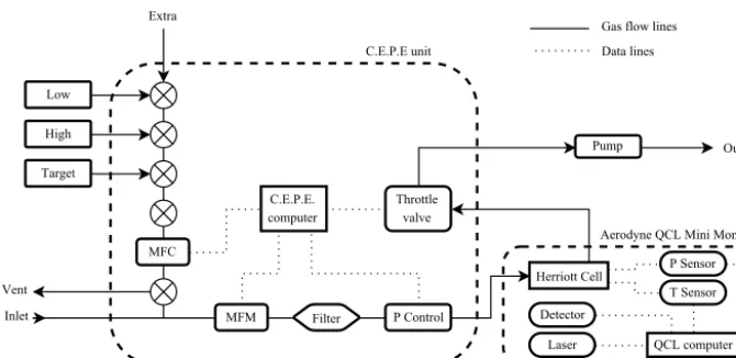
The QCLAS is mounted on a rack inside the cabin of the FAAM aircraft, with a rearward-facing, 3/800outer diameter, stainless steel inlet inserted through a customised window blank (Avalon Aero Ltd., UK). The sample flow line consists of Swagelok 1/400 outer diameter PFA Teflon tubing, partly encased within the inlet, and forming a pressure seal via a bored-through Swagelok 3/800 to 1/400 reducing union. Fig-ure 1 shows a schematic of the QCLAS air sampling system including the configuration for delivering calibration gas to the sample cell. The sample flow line is∼2.5 m in length from the inlet tip to the pressure controller. Sample flow rate is measured using a 30 SLPM (standard litres per minute) mass flow meter (M10MB01334CS3BV, MKS Instruments UK Ltd, UK), placed directly upstream of a 0.5 µm sintered particle filter (SS-4F-05, Swagelok, USA).
The choice of sample cell pressure is a balance between two effects: higher pressures increase the absorption, thus improving the signal-to-noise ratio of the measurement, whilst pressure broadening of the spectral lines increases spectral overlap and line mixing (as discussed by Zahniser et al., 1995). Airborne operation is also complicated by the large variation in inlet pressures typically encountered over the course of a flight (down to∼250 hPa at 10 km altitude).
Figure 1. Schematic showing the QCLAS air sampling and data handling systems. The C.E.P.E. (calibration, exhaust, power and electronics) unit and the Aerodyne QCL mini-monitor enclosures are represented by dashed boxes around the components they contain. The calibration cylinders are labelled “low”, “high” and “target”. The flow rate of the calibration gas is controlled by the MFC (mass flow controller), and the flow rate into the instrument is monitored by the MFM (mass flow meter). The optical components associated with the alignment of the laser beam are not shown.
altitude. A cell pressure of 68.9±3.6 hPa (at 1σ )was used during the GAUGE and MAMM campaigns.
Air is pulled through the system using a single stage scroll pump (Edwards XDS10, Edwards, UK). A throttle valve (253B-1-40-1, MKS Instruments UK Ltd, UK) positioned between the sample cell outlet and the pump inlet is used to control the flow rate through the system. This again is a bal-ance between the desire to decrease the instrument response time, favouring a faster flow rate, and the desire to reduce the total pressure drop between the inlet and the sample cell, favouring a slower flow rate. Throughout the GAUGE and MAMM campaigns the valve was set to 18 % of its fully open position, resulting in a constant mass flow rate of 1.43±0.21 SLPM (at 1σ )down to inlet pressures of∼380 hPa. At lower inlet pressures both the mass flow rate and the cell pressure were reduced.
Laboratory tests were performed to establish the effect of cell pressure changes on the mole fractions retrieved when sampling a compressed air cylinder. The variability in re-trieved mole fraction was found to be no greater across cell pressures typically encountered during high altitude fly-ing (inlet pressures below 380 hPa; cell pressures down to ∼46 hPa) than across the range experienced during low alti-tude flying (inlet pressures above 380 hPa; cell pressures be-tween 65 and 76 hPa). It was therefore deemed unnecessary to filter data according to the absolute cell pressure value. However, rapid changes in pressure were found to impact upon the retrieved mole fractions; consequently data were re-moved whenever the 10 s standard deviation in cell pressure exceeded 0.1 Torr (13.3 Pa).
The response time of the system was determined in the laboratory (at 1017 hPa inlet pressure) by overflowing the in-let with N2 from a compressed gas cylinder. The e-folding
time of the system was determined using an exponential fit
to the decay in retrieved mole fractions and was found to be 0.68±0.12 s (mean±1σ ). The inlet lag time was given by the time between turning on the N2flow and the first drop in
retrieved mole fractions. In this laboratory test it was found to be in the range 2–3 s; however, we expect this lag time to decrease with altitude (up to∼380 hPa) as the volumetric flow rate of the system scales inversely with air density (for a constant mass flow rate).
In principle the Beer–Lambert relationship described above can be used to retrieve absolute mole fractions. How-ever, in-flight calibration is commonly used to account for instrumental drift when using optical-based measurements (e.g. O’Shea et al., 2013b; Santoni et al., 2014), as external variables such as temperature and pressure can undergo sig-nificant variation during a flight. Our system employs three calibration standards to scale the data and assess instrument performance, as described in Sect. 3.1.
The three calibration standards are stored in 10 L carbon fibre hoop-wrap cylinders (BFC 124-136-002, Aluminium Alloy 7060, Luxfer, UK), which are filled to ∼300 bar and mounted to the QCLAS rack. Each cylinder is fitted with a high-pressure brass valve (C215, Rotarex, Luxem-bourg), screwed into the cylinder collar using PTFE (poly-tetrafluoroethylene) tape. An all brass adapter connects this to instrument-grade stainless steel tubing of 1/800 outer
from an external cylinder). The flow rate is set using a mass flow controller (1179A01314CS1BV, MKS Instruments UK Ltd, UK) to provide an overflow of calibrant at the inlet (up-stream of the mass flow meter).
2.4 Water vapour correction
The influence of water vapour on spectral retrievals can be very significant (e.g. Allen et al., 2014), particularly given the wide range of natural water vapour concentrations typically encountered over the course of a flight (from a small fraction of a percent to many percent in the troposphere alone). To ensure comparability between measurements made at differ-ent humidity levels it is necessary to remove this effect and report dry mole fractions.
Many opt to circumvent the need to correct for this in-fluence by drying the sample air before it enters the instru-ment, often using a combination of Nafion gas dryers and dry ice traps (e.g. Daube et al., 2002; Peischl et al., 2010; Santoni et al., 2014). The advantage of this approach is obvi-ous, as any empirically derived correction for the influence of water vapour will contribute, often significantly, to the overall uncertainty of the measurements. However, there are several disadvantages associated with drying the sample, as discussed in detail by Rella et al. (2013). Of particular rel-evance for the QCLAS system described here are the issues associated with increasing the pressure drop across the inlet system, increasing the residence time in the inlet system and the logistical problems of supplying dry ice to remote field locations and transporting it in a sealed cabin environment.
In cases such as this, where the sample is not dried, an empirical correction must be derived in order to account for the water vapour influence. Typically this involves applying a scale factor to the retrieved mole fractions, with its form and coefficients determined through laboratory experiment. Rella et al. (2013), O’Shea et al. (2013b) and Zellweger et al. (2012) employ this approach across a variety of spec-troscopic instruments. However, a recently added feature of the TDLWintel software allows the effect of line broadening (in addition to sample dilution) due to the presence of wa-ter vapour to be included in the spectroscopic retrieval itself. Instrument-specific coefficients quantifying the broadening due to water vapour must be derived empirically for each species. These coefficients are equal to the dimensionless ra-tio of the line broadening due to water vapour pressure to the line broadening due to dry air pressure. Water-corrected mole fractions are then determined by first retrieving the wa-ter vapour mole fraction, then combining this result with the appropriate water broadening coefficients in the retrieval of the other species.
Here we compare the effectiveness of these two ap-proaches in the case of the QCLAS. Such a comparison of these two methods is instructive to other experimentalists that may seek to apply similar corrections. Both approaches
require empirical (laboratory) data, which can be obtained simultaneously for direct comparison.
As the empirical coefficients required by both methods can be determined using the same experiment, and TDLWintel retains the measured raw spectral data, it was possible to per-form this comparison by reanalysing the same data set, ei-ther deriving a scale factor to post-process the data or vary-ing the way in which the water vapour influence was treated in the retrieval. The data here were gathered in four separate laboratory experiments, each using an identical experimen-tal setup to that employed by O’Shea et al. (2013b), who provide a full description. In summary, dry compressed air was humidified to a variety of different water vapour mole fractions, spanning the range of 0–2 % typically measured in flight. Between each measurement of humid air, a dry refer-ence was sampled, using a dry ice trap to reduce the sample dew point to less than−60◦C. It should be noted that by
re-drying the air downstream of the humidifier we accounted for any dissolution of gases in the humidifier and the temperature dependence of this effect.
The first approach used the following relationship to scale the measurements of the wet sample to corresponding dry mole fractions
Xdry= Xwet a+bH2O
, (2)
where Xwet and Xdry are the raw and the scaled
water-corrected mole fractions respectively for speciesX, and H2O
represents the retrieved mole fraction of water vapour. Coef-ficientsaandbwere derived by performing a weighted least orthogonal distance regression ofXwet/Xdryas a function of
H2O for data from all four experiments.
The empirical values for the QCLAS were found to bea= 1.00096, b= −0.0154563 %−1 for N2O and a=1.00071, b= −0.0136929 %−1for CH4. The uncertainties associated
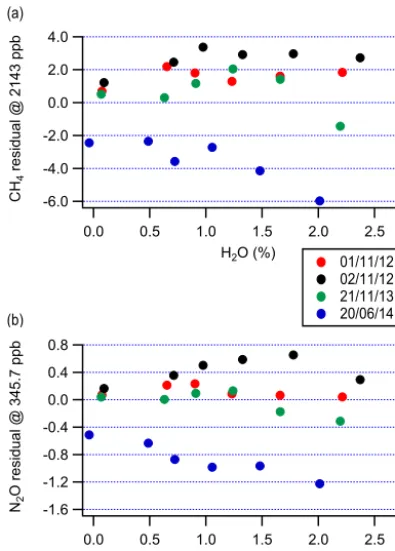
with these values can be quantified by the residuals of this re-gression for CH4and N2O, shown in Fig. 2. The RMS (root
mean square) values for these residuals are 2.5 and 0.50 ppb for CH4and N2O respectively.
It is apparent from Fig. 2 that substantially different be-haviour was observed on 20 June 2014 when compared to the three other experiments. This is likely to be associated with a lack of long-term stability in the retrieval of H2O mole
frac-tion, as indicated by the drift in the average retrieved H2O
mole fraction during the dry runs seen in Fig. 2. As this is a measurement of very dry air (less than−60◦C dew point),
this drift can be assumed to represent the variability in the baseline intensity in the region of the H2O absorption line,
likely resulting from very small changes in the optical align-ment and/or pathlength. This subtle variability in baseline intensity then manifests as systematic variability in the accu-racy of the retrieved H2O mole fractions. The consequence of
-6.0 -4.0 -2.0 0.0 2.0 4.0
CH
4
residual @ 2143 ppb
2.5 2.0 1.5 1.0 0.5 0.0
H2O (%) (a)
(b)
01/11/12 02/11/12 21/11/13 20/06/14
-1.6 -1.2 -0.8 -0.4 0.0 0.4 0.8
N2
O residual @ 345.7 ppb
2.5 2.0 1.5 1.0 0.5 0.0
H2O (%)
Figure 2. Residual error due to the influence of water vapour for
the retrieval of (a) CH4and (b) N2O after applying an empirically
derived scale factor to correct the data. Data from four identical experiments are shown; the residuals are calculated as the product of the fractional error for each measurement and the average mole fraction for the dry measurements taken during all four experiments.
The second, spectroscopic, water vapour correction method used the water broadening function in TDLWintel to correct for the influence of water vapour. Reanalyses of the raw spectra were performed using a variety of different water broadening coefficients in the retrieval. For each coef-ficient, the difference between the retrieved wet mole frac-tion and the corresponding dry measurement was calculated at every water vapour level used during the four experiments. The RMS difference for each coefficient, averaged over the entire data set, is shown in Fig. 3. It can be seen that the cor-rection performed best using water broadening coefficients of 1.6 and 1.8 for CH4 and N2O respectively. These
opti-mal coefficients resulted in RMS differences between corre-sponding wet and dry measurements of 1.6 ppb for CH4and
0.32 ppb for N2O; these are the values used to determine the
contribution of uncertainty in this water vapour correction to the total measurement uncertainty of the instrument.
It was thus concluded that in this case a better correc-tion for the influence of water vapour was obtained using the spectroscopic correction performed by the TDLWintel software than was achieved by scaling the wet mole frac-tions according to Eq. (2). There are two potential factors that could explain the improved performance of the spectroscopic
12 10 8 6 4 2 0
RMS difference
2.2 2.0
1.8 1.6
Water broadening coefficient
2.4 2.0 1.6 1.2 0.8 0.4 0.0
CH4
N2O
Figure 3. RMS (root mean square) difference between the retrieved wet mole fractions and the corresponding dry measurements for
CH4and N2O, as a function of water broadening coefficient. These
RMS values are determined using data taken over the full
experi-mental range of H2O mole fraction during all four identical
experi-ments.
method over the scale factor method. Firstly, because the spectroscopic correction determines the water vapour pres-sure broadening relative to the dry air prespres-sure broadening, it implicitly accounts for changes in absolute water vapour pressure associated with corresponding changes in measured sample cell pressure. In contrast, the scale factor method us-ing Eq. (2) relies only on the retrieved mole fraction of water vapour and so fails to account for any increase or decrease in water vapour pressure broadening at higher or lower cell pressures.
Secondly, in the scale factor method, drift in the uncali-brated water vapour mole fraction measurements propagates directly via Eq. (2) into a systematic error in the water-corrected mole fraction for both CH4 and N2O (Xdry). In
the spectroscopic method, inaccuracies in the measurement of water vapour mole fraction instead impact upon the sub-sequent retrieval of CH4and N2O by affecting the fitting of
the Voigt line profile. Although inaccurately calculated wa-ter vapour line broadening will change the retrieved mole fraction using the spectroscopic method, because the water vapour broadening is just one of several parameters con-straining the spectral fit, inaccuracy resulting from this effect will be manifest in part as a reduction in the goodness of fit (spectral residual). Hence the spectroscopic method is less sensitive to any potential drift in the retrieval of water vapour mole fraction than the scale factor method.
3 Data quality
Systematic instrumental error associated with changes in ex-ternal variables such as temperature and pressure can be com-pensated for by repeated sampling of calibration gas. During airborne sampling an instrument is exposed to rapid changes in these variables over a wide range of values; hence regular calibration is required.
In this section we first describe the calibration procedure used during the two campaigns and explain the rationale be-hind it. We then seek to diagnose and understand the sources of systematic error which remain uncaptured by this calibra-tion. Finally, we describe an alternative calibration procedure designed to better address these key sources of error and eval-uate the effect of both methods on the overall data quality. 3.1 Original calibration procedure
The in-flight calibration procedure employed throughout the GAUGE and MAMM campaigns was in principle similar to that described by O’Shea et al. (2013b). The data were scaled using two cylinders of known composition, traceable to the WMO greenhouse gas scale (WMO, 2009), whose mole fractions spanned the normal measurement range for N2O
and CH4. By sequentially pumping gas from these cylinders
through the system and comparing the retrieved mole frac-tions to their WMO-traceable values, two reference points could be established for the QCLAS on the WMO scale. By assuming a linear relationship, the “true” mole fraction corre-sponding to each retrieved QCLAS mole fraction was given by interpolating the scale between the two reference points. For each calibration a scale factor (Mx) and zero offset (Cx)
were found using
Mx=
Xhigh,WMO−Xlow,WMO Xhigh,meas−Xlow,meas
, (3)
Cx=Xhigh,WMO−MxXhigh,meas, (4)
where Xhigh,WMO and Xlow,WMO are the “true”
WMO-traceable mole fraction values, andXhigh,meas andXlow,meas
are the measured mole fraction values, for the high and low calibration cylinders respectively for a given speciesX.
These two cylinders were sampled sequentially on an ap-proximately hourly basis and the values forMxandCxwere
linearly interpolated between calibrations. The raw data were then calibrated by applying
Xcal(t )=Mx(t )Xraw(t )+Cx(t ). (5)
In order to check that both interpolation between the two cylinder mole fraction values and temporal interpolation between hourly calibrations were justified, a third WMO-traceable “target” cylinder containing intermediate CH4and
N2O mole fractions was measured approximately mid-way
between the hourly high–low span calibrations. Applying the above calibration to this target cylinder measurement and
2400
2200
2000
1800
CH
4
raw (ppb)
12:30
15/05/2014 13:00 13:30
UTC
1
Calibration index
CH4 raw Target High Low
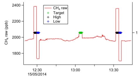
Figure 4. A selection of raw CH4 data from flight B848, over-laid with calibration index markers to highlight the hourly calibra-tion cycle. The target cylinder measurement (green markers) is per-formed approximately mid-way between the high–low span cylin-der measurements (black and blue markers respectively) used to cal-ibrate the data to the WMO scale.
140
120
100
80
60
Raw QCLAS CH
4
offset (ppb)
12:00 15/05/2014
13:00 14:00 15:00 16:00 17:00
UTC
Figure 5. The offset between the raw QCLAS CH4data and the calibrated FGGA data (used here as our reference) during flight B848. Gradients of over 30 ppb in less than 10 min can be seen to be present.
comparing the resulting calibrated mole fractions with the WMO-traceable values for the cylinder enabled errors as-sociated with this method to be quantified. Raw CH4 data
demonstrating a typical calibration cycle are shown in Fig. 4. This calibration procedure was designed to remove lin-ear drifts acting over timescales of the order of the inter-calibration time, here approximately 1 h. However, analy-sis of the difference in CH4 mole fraction between the
raw QCLAS data and the calibrated data from the on-board FGGA frequently showed gradients of over 30 ppb in timescales of less than 10 min, as shown for flight B848 in Fig. 5. The FGGA on board the FAAM aircraft has previ-ously been shown not to exhibit any significant systematic errors on this timescale (O’Shea et al., 2013b), suggesting that these gradients represent a source of systematic error in the QCLAS data. Note that although we have compensated here for the lag time between the two instruments using the correlation between the two CH4data sets, large deviations
140
120
100
80
60
Raw QCLAS CH
4
offset (ppb)
1000 800
600 400
Static Pressure (hPa) QCLAS-FGGA Target cylinder High cylinder Low cylinder
Figure 6. The offset between the raw QCLAS CH4measurements and both the corresponding calibrated FGGA data and the known contents of the target, high and low calibration cylinders during flight B848, shown as a function of static pressure. Although the absolute magnitude of the offset differs for these four different mea-surements, the same broadly repeatable pattern is exhibited by each of them.
as a result of small differences in the measurement time of large CH4enhancements.
Figure 6 shows the same CH4data from flight B848
plot-ted as a function of static pressure, as measured by the air-craft’s RVSM (reduced vertical separation minimum) sys-tem. It can be seen that a broadly repeatable pattern exists as a function of pressure, which was found to dominate vari-ability in the raw QCLAS CH4data offset with respect to the
FGGA over the course of the flight. The same pattern is also exhibited by the offset of the calibration cylinder measure-ments from the nominal values of the cylinders (also shown), although the absolute value of this offset clearly differs be-tween the cylinders. Similar patterns were observed for the cylinder measurements of N2O, and across other flights
dur-ing the two campaigns.
The fact that this variation with pressure can be observed in both the raw sample data and the measurement of dry cal-ibration air confirms that errors in the water vapour correc-tion cannot be responsible. A leak (ingress) into the system also appears implausible, as one would expect this to have the opposite effect on the high and low cylinder measure-ments, pulling both towards the mole fractions of CH4and
N2O present in the aircraft cabin. Santoni et al. (2014) warn
of issues associated with fluctuations in sample cell pressure. However, the offsets in retrieved QCLAS mole fractions ob-served here were found to exhibit no dependence on either sample cell pressure, sample cell temperature or the rate of change for these variables (as recorded by the pressure and temperature sensors within the sample flow).
120 110 100 90 80
Raw QCLAS CH
4
offset (ppb)
950 900 850
Cabin pressure (hPa)
120 110 100 90 80
Raw QCLAS CH
4
offset (ppb)
1000 800 600 400
External pressure (hPa)
(a) 4 (b)
2
0
-2
-4
Raw QCLAS N
2
O offset (ppb)
950 900 850
Cabin pressure (hPa)
(c) 4 (d)
2
0
-2
-4
Raw QCLAS N
2
O offset (ppb)
1000 800 600 400
External pressure (hPa)
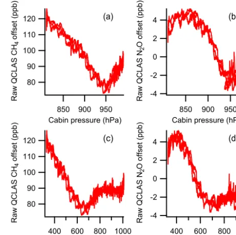
Figure 7. The offset between the raw retrieved QCLAS mole frac-tions and the known content of a target cylinder, sampled continu-ously during three separate deep profiles during flight B903. Panels (a) and (b) shown the offset as a function of the pressure inside the
cabin, for CH4and N2O respectively. Panels (c) and (d) show the
offset as a function of external static pressure (also for CH4 and
N2O respectively).
The temperature of the cabin air was also recorded as it entered the outer enclosure of the QCLAS, but this again ex-hibited no clear correlation with the CH4 data offset. The
pressure inside the cabin, however, was not recorded dur-ing the 2014 campaigns. Subsequent test flights, described in Sect. 3.2 below, suggest that it was variability in this quan-tity that caused the large gradients in CH4offset described
above.
3.2 Influence of cabin pressure
In April 2015 we performed a test flight (B903) designed to further understanding of the underlying issues behind the large gradients in QCLAS CH4 data described in Sect. 3.1
above. This time cabin pressure data were available through-out the flight, and three deep profiles were performed whilst the QCLAS sampled compressed air from a calibration cylin-der. The first deep profile occurred at the beginning of the flight, whilst the other two were performed∼2.5 h later.
Figure 7 shows the offset in retrieved CH4 and N2O
120 110 100 90 80
Raw CH
4
offset (ppb)
14:00
30/04/2015 14:15 14:30 14:45
UTC 1000
950
900 850
800
Cabin pressure (hPa)
1000
800
600
400
External pressure (hPa)
6 4 2 0 -2 -4
Raw N
2O offset (ppb)
Figure 8. Time series from flight B903, showing the offset between the raw retrieved QCLAS mole fractions and the known content of the target cylinder being sampled. Cabin pressure and external static pressure are also shown to illustrate the systematic nature of the offset during two consecutive profiles.
for both CH4and N2O, the raw QCLAS measurement offset
does not change when the cabin pressure is constant, even when the external pressure is varying, strongly suggests that cabin pressure variability is the primary cause of the large gradients in this offset observed throughout the GAUGE and MAMM campaigns in summer 2014.
A time series of the retrieved mole fraction offsets for the final two profiles is shown in Fig. 8. The influence of chang-ing cabin pressure on these retrieved mole fractions can be characterised as a small-scale oscillation superimposed on a larger-scale gradient. This large-scale gradient appears to be very consistent across the three profiles (see also Fig. 7), whereas the small-scale oscillations are not so repeatable.
The likely pathway through which cabin pressure can in-fluence the retrieved mole fractions is through its effect on baseline intensity in the spectral regions close to the absorp-tion lines. There are two potential components to this: the effect of changing absorption in the open path section of the laser and the effect of changing pressure on the alignment of, and spacing between, the instrument’s optical components.
To investigate the effect of varying the open path absorp-tion, a further test flight was conducted whilst flowing dry
nitrogen through the laser beam enclosure. A simulation was also performed, where open path CH4and N2O absorption
were included in the spectral fit for the range of cabin pres-sures encountered during flight B903, to assess the impact on the retrieved mole fractions. Both of these tests indicated that varying open path absorption contributed negligibly to the observed gradients in retrieved mole fraction over the range of cabin pressures experienced during these flights. Hence we conclude that these gradients are more likely at-tributable to small changes in optical alignment/spacing as-sociated with cabin pressure variation.
3.3 Pressure-differentiated calibration procedure
As the short-term (of order minutes) instrumental drift with pressure had a greater effect in degrading measurement pre-cision than any longer-term (of order hours) drift with time, the data were reanalysed using an alternative calibration pro-cedure, designed to reduce the impact of this issue on the overall accuracy of the calibrated measurements. As there were no cabin pressure data available for the GAUGE and MAMM campaigns in summer 2014, it was necessary to use the external static pressure from the aircraft’s RVSM system as a proxy. This approach is justified by the strong correla-tion between cabin pressure and external pressure and by the results in Sect. 3.4 below.
In this approach values ofMx(t ) andCx(t )for sections
of flight at broadly equivalent pressure levels (defined here as a range of variability less than 15 hPa for a period longer than 2 min) were interpolated between any calibrations con-ducted at a pressure within 15 hPa of the average pres-sure during that section. Profile data, along with all data at pressure levels where no calibrations were performed, were flagged as poor quality and removed from the analysis. This pressure-differentiated calibration method has the disadvan-tages of both reducing the amount of calibrated data for the campaigns by 54 % and potentially inducing errors associ-ated with long-term instrumental drift, as data can be sep-arated from the corresponding calibration(s) by up to 5 h. The effect on the overall data quality of using this pressure-differentiated calibration procedure is discussed and com-pared in Sect. 3.4.
It was also found that large roll angles (∼20◦or over), as-sociated with sharp turns of the aircraft, produced short-term deviations in retrieved CH4and N2O mole fractions, evident
in both the raw and calibrated data. It is likely that this ef-fect is a consequence of slight alignment changes (similar to Sect. 3.2 above) caused by the centrifugal force of the turn (no relationship with cabin pressure variability was found). Whilst this effect was clearly secondary to the pressure-dependent variability described above, producing CH4
reduced-Table 1. Mean and standard deviation of the difference between QCLAS 1 Hz target cylinder measurements and the nominal cylinder values
and the difference between the 1 Hz QCLAS and the corresponding 1 Hz FGGA sample CH4measurements, using both the original and
pressure-differentiated calibration methods.
QCLAS–target difference (ppb) QCLAS–FGGA
difference (ppb)
N2O CH4 CH4
Calibration method Mean 1σ Mean 1σ Mean 1σ
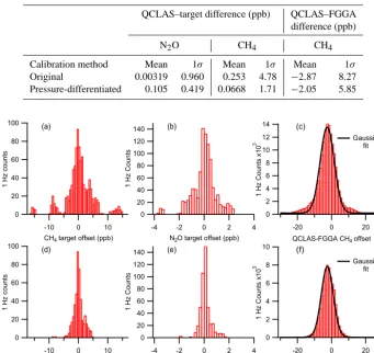
Original 0.00319 0.960 0.253 4.78 −2.87 8.27
Pressure-differentiated 0.105 0.419 0.0668 1.71 −2.05 5.85
10
8
6
4
2
0
1 Hz Counts x10
3
-20 0 20
QCLAS-FGGA CH4 offset
Gaussian fit 14
12 10 8 6 4 2 0
1 Hz Counts x10
3
-20 0 20
QCLAS-FGGA CH4 offset
Gaussian fit 100
80
60
40
20
0
1 Hz counts
-10 0 10
CH4 target offset (ppb)
140 120 100 80 60 40 20 0
1 Hz Counts
-4 -2 0 2 4
N2O target offset (ppb)
100
80
60
40
20
0
1 Hz counts
-10 0 10
CH4 target offset (ppb)
140 120 100 80 60 40 20 0
1 Hz Counts
-4 -2 0 2 4
N2O target offset (ppb)
(a) (b) (c)
(d) (e) (f)
Figure 9. Histograms showing the offset between the calibrated 1 Hz QCLAS measurements and both the corresponding target cylinder values and the corresponding FGGA sample measurements. Panels (a)–(c) show histograms for data calibrated using the original method; in comparison, panels (d)–(f) show the corresponding histograms using the pressure-differentiated calibration method. It can be seen here that the pressure-differentiated method results in the removal of many of the outlying target cylinder measurements. In addition, the Gaussian fit
to the QCLAS–FGGA CH4offset is also improved by the pressure-differentiated calibration method (f) relative to the original method (c).
quality data associated with high roll angles. The application of this filter reduces the total size of the raw data set by only 7 %.
3.4 Results and discussion
The performance of the QCLAS can be assessed both by comparing the calibrated target cylinder measurements to their corresponding WMO-traceable values and by compar-ing the calibrated 1 Hz CH4sample data with the
correspond-ing measurements from the on-board FGGA. No other instru-ments on board the FAAM aircraft measured N2O during the
GAUGE or MAMM campaigns, so a direct comparison of sample N2O mole fractions cannot be made here. Table 1
summarises these results for both the original calibration method described in Sect. 3.1 and the pressure-differentiated calibration method described in Sect. 3.2.
It can be seen from the table that using the pressure-differentiated calibration method significantly improves the accuracy of the QCLAS, both during target cylinder mea-surements and sample mode. In particular, the standard de-viations in QCLAS–target and QCLAS–FGGA differences are substantially reduced compared to the equivalent values produced using the original calibration method. The WMO recommends compatibility between different analyses within 2 ppb for CH4 and 0.1 ppb for N2O (WMO, 2013). The
fraction of data within these ranges for both the QCLAS– target and QCLAS–FGGA differences using both methods is shown in Table 2. Here again it can be seen that the pressure-differentiated calibration method produces superior results.
Figure 9 shows the offset between the calibrated 1 Hz QCLAS target cylinder measurements and the known content of the cylinder, as histograms for both CH4and N2O. It can
Table 2. The fraction of 1 Hz data within the WMO compatibil-ity recommendations for QCLAS target cylinder measurement and QCLAS–FGGA sample measurement, using both the original and pressure-differentiated calibration methods.
QCLAS–target QCLAS–FGGA
Calibration method N2O CH4 CH4
Original 0.149 0.519 0.292
Pressure-differentiated 0.309 0.765 0.361
Table 3. Allan precision for QCLAS measurement of CH4 and
N2O, both during ambient in-flight sampling and whilst sampling a
compressed air cylinder in the laboratory, given for averaging times of 1, 10 and 108 s.
1σAllan precision (ppb)
1 s 10 s 108 s
Flight Lab Flight Lab Flight Lab
CH4 0.52 0.48 0.31 0.17 0.23 0.12
N2O 0.11 0.12 0.074 0.044 0.042 0.029
using the pressure-differentiated calibration method result from the removal of outlying data associated with the pres-sure effect discussed in the previous section. Also shown are histograms of the QCLAS–FGGA offset for 1 Hz CH4
sam-ple data, which provide further evidence of the superior per-formance of the pressure-differentiated calibration method. The data produced using the original calibration method are clearly far less well represented by a Gaussian fit; this is to be expected in the presence of a systematic effect such as that described in Sect. 3 above. In contrast, the Gaussian shape of the pressure-differentiated data is consistent with a random error distribution for both instruments.
The instrument precision can be quantified using the Al-lan variance technique (Werle et al., 1993). Table 3 presents the 1σ Allan precision (over 1, 10 and 108 s) for CH4and
N2O, both in a laboratory environment whilst sampling a
compressed air cylinder and in flight during a period of am-bient background sampling. These results are similar to those of Santoni et al. (2014), with in-flight 1 Hz precisions here of 0.52 ppb for CH4and 0.11 ppb for N2O.
Finally, a nominal uncertainty for the data can be calcu-lated using the known uncertainties from the water vapour correction experiment, the calibration of the target cylinder to the WMO-scale and the in-flight target measurements. Ta-ble 4 contains these values for both CH4and N2O using the
pressure-differentiated calibration method. The nominal to-tal uncertainties for CH4and N2O are±2.47 and±0.54 ppb
respectively.
Table 4. Known component and nominal total uncertainties for
the QCLAS measurement of CH4 and N2O, calibrated using the
pressure-differentiated method.
1σuncertainty (ppb)
Water vapour Target standard In-flight target Total
correction calibration measurements
CH4 1.63 0.77 1.71 2.47
N2O 0.32 0.11 0.42 0.54
Figure 10. Aircraft flight track for flight B868, coloured by N2O mole fraction. Average wind speeds and directions taken over 60 s are shown as a wind barbs (using the convention where each full barb represents a wind speed of 10 knots). Selected HYSPLIT back
trajectories are shown for a region of enhanced N2O (black) and
a contrasting region of lower N2O (grey). Map data: Google, SIO,
NOAA, US Navy, NGA, GEBCO, Landsat.
4 Case study
The GAUGE project aims to provide top-down greenhouse gas emission estimates for the UK, which can be used to val-idate the bottom-up inventory-based estimates required by UK and international legislation. As part of this approach, the use of aircraft data is planned in combination with mass balance techniques (Karion et al., 2013; O’Shea et al., 2014a; Peischl et al., 2015) to estimate regional greenhouse gas emissions. Such analysis is beyond the scope of this tech-nical study; however, we present QCLAS data from a single flight here as exemplars of typical flight data, providing con-text with regard to scientific case studies which may use this new airborne data set.
Flight B868 was designed to incorporate upwind and downwind sampling over north-western England to provide a data set for a mass balance case study. This region con-tains several large urban areas (Manchester, Liverpool, Leeds and Sheffield) and also includes several areas of agricultural activity, known to be an important anthropogenic source of N2O (Syakila and Kroeze, 2011). The flight track, coloured
by N2O mole fraction, is shown in Fig. 10. The wind speed
ac-cording to the standard convention where each full barb rep-resents a wind speed of 10 knots. Selected Lagrangian back trajectories using the HYSPLIT (Hybrid Single-Particle La-grangian Integrated Trajectory) model (Draxler and Hess, 1998) are also shown (representing around 24 h track across the UK mainland in the figure). These trajectories were initi-ated using endpoints and trajectory end times selected along the flight track and modelled with full vertical dynamics us-ing Global Data Assimilation System 1◦resolution data.
It can be seen that the N2O mole fractions measured in
the north-west of the domain were enhanced relative to those in the south-east. A relatively consistent south-easterly wind direction (both measured and seen in the trajectories) sug-gests that this enhancement may enable the use of a mass balance technique to estimate the N2O flux from an area
be-tween this downwind transect and the corresponding upwind measurements using the techniques described by O’Shea et al. (2014a). This requires suitable investigation of the neces-sary assumptions, which is beyond the scope of this simple example.
It is also striking that there is a relative contrast in the south-west area of the domain, with N2O mole fractions
around 328 ppb (compared with 330 ppb in the north-west). The potential reasons for this small contrast, in terms of air-mass history, may be explained by considering both the tra-jectories and the wind barbs. The tratra-jectories from the north-west domain show recent transport at low altitude (below 1 km) over Greater Manchester and the north-west conur-bation, whereas south-west trajectories pass over more rural areas. This appears counterintuitive, as we expect the agri-cultural sector to be the primary contributor towards N2O
emissions in this region. However, the wind barbs (which represent real measurements) show that there is a complex divergence in the wind field in the south-west domain, per-haps indicative of a localised sea-breeze circulation that can-not be expected to have been captured at the resolution of the meteorological data that were used to initialise the HYS-PLIT trajectories. This sea-breeze circulation could suggest recirculation of maritime air and hence dilution of any mod-erately enhanced air arriving on the prevailing wind from the east. The differing localised dynamics and air-mass histories of the two domains may explain the observed contrast. Fur-ther analysis of this may form the basis of future work and this limited example demonstrates the utility of aircraft data in understanding local and regional air-mass characteristics.
5 Conclusions
A quantum cascade laser absorption spectrometer was used to measure N2O and CH4on board the FAAM aircraft
dur-ing the GAUGE and MAMM campaigns in summer 2014. A relationship between QCLAS measurement error and cabin pressure was found, and a new calibration procedure was adopted to minimise the impact of this effect on the final data.
Using this pressure-differentiated calibration method, total uncertainties of±2.47 ppb and±0.54 ppb were obtained for the measurement of CH4and N2O respectively.
The sample air was not dried prior to measurement, so a correction for the influence of water vapour on the retrieved mole fractions was required. The performance of two dif-ferent water vapour correction methods was compared using data from four separate experiments. It was found that the best results were obtained using the water broadening func-tion in the TDLWintel software, which included the effects of water broadening on the CH4and N2O absorption lines
di-rectly in the mole fraction retrieval. Experimentally derived coefficients for the ratio of water vapour broadening to air broadening of 1.6 and 1.8 were found to give the best results for CH4and N2O respectively.
Overall instrument performance is found to be broadly comparable with similar studies (e.g. O’Shea et al., 2013b; Santoni et al., 2014) when the pressure-differentiated calibra-tion procedure is used. However, this has the disadvantage of removing 54 % of the measured sample data, including all data during vertical profiles, which are frequently of sci-entific interest. A priority for improvement is to prevent the large short-term drifts in measurement error that necessitate the removal of these data. One potential solution would be to enclose the instrument within a pressure-sealed container. The feasibility of practically implementing this solution on board the FAAM aircraft is currently being studied.
Acknowledgements. The authors would like to thank everyone at
FAAM and the numerous people at Avalon Aero and Directflight who assisted with the logistics of installing the QCLAS on the aircraft. J. R. Pitt is in receipt of a NERC CASE studentship in partnership with FAAM, grant number NE/L501/591/1, supervised by G. Allen. This work was supported by the NERC projects: GAUGE (Greenhouse gas UK and global emissions), grant number NE/K002279/1, and MAMM (Methane and other greenhouse gases in the Arctic: measurements, process studies and modelling), grant number NE/I029161/1. We are also grateful to the Norwe-gian Research Council, which partly funded the 2014 MAMM flights through the MOCA (Methane emissions from the Arctic Ocean to the atmosphere: present and future climate effects) project.
Edited by: A. Hofzumahaus
References
Allen, G., Illingworth, S. M., O’Shea, S. J., Newman, S., Vance, A., Bauguitte, S. J.-B., Marenco, F., Kent, J., Bower, K., Gal-lagher, M. W., Muller, J., Percival, C. J., Harlow, C., Lee, J., and Taylor, J. P.: Atmospheric composition and thermodynamic re-trievals from the ARIES airborne TIR-FTS system – Part 2: Val-idation and results from aircraft campaigns, Atmos. Meas. Tech., 7, 4401–4416, doi:10.5194/amt-7-4401-2014, 2014.
integrated-cavity-output spectroscopy, Appl. Phys. B-Lasers O., 75, 261–265, doi:10.1007/s00340-002-0971-z, 2002.
Chen, H., Winderlich, J., Gerbig, C., Hoefer, A., Rella, C. W., Crosson, E. R., Van Pelt, A. D., Steinbach, J., Kolle, O., Beck, V., Daube, B. C., Gottlieb, E. W., Chow, V. Y., Santoni, G. W., and Wofsy, S. C.: High-accuracy continuous airborne
measure-ments of greenhouse gases (CO2and CH4) using the cavity
ring-down spectroscopy (CRDS) technique, Atmos. Meas. Tech., 3, 375–386, doi:10.5194/amt-3-375-2010, 2010.
Ciais, P., Sabine, C., Bala, G., Bopp, L., Brovkin, V., Canadell, J., Chhabra, A., DeFries, R., Galloway, J., Heimann, M., Jones, C., Quéré, C. Le, Myneni, R. B., Piao, S., and Thornton, P.: Carbon and Other Biogeochemical Cycles, in: Climate Change 2013: The Physical Science Basis. Contribution of Working Group I to the Fifth Assessment Report of the Intergovernmental Panel on Climate Change, edited by: Stocker, T. F., Qin, D., Plattner, G.-K., Tignor, M., Allen, S. K., Boschung, J., Nauels, A., Xia, Y., Bex, V., and Midgley, P. M., Cambridge University Press, Cambridge, United Kingdom and New York, NY, USA, 465– 570, 2013.
Crosson, E. R.: A cavity ring-down analyzer for measuring atmo-spheric levels of methane, carbon dioxide, and water vapor, Appl. Phys. B-Lasers O., 92, 403–408, doi:10.1007/s00340-008-3135-y, 2008.
Daube, B. C., Boering, K. A., Andrews, A. E., and Wofsy, S. C.:
A High-Precision Fast-Response Airborne CO2 Analyzer for
In Situ Sampling from the Surface to the Middle Stratosphere, J. Atmos. Ocean. Tech., 19, 1532–1543, doi:10.1175/1520-0426(2002)019<1532:AHPFRA>2.0.CO;2, 2002.
Draxler, R. R. and Hess, G. D.: An Overview of the HYSPLIT_4 Modelling System for Trajectories, Dispersion, and Deposition., Aust. Meteorol. Mag., 47, 295–308, 1998.
Ebi, K. L. and McGregor, G.: Climate change, tropospheric ozone and particulate matter, and health impacts., Environ. Health Persp., 116, 1449–1455, doi:10.1289/ehp.11463, 2008. Fraser, A., Palmer, P. I., Feng, L., Boesch, H., Cogan, A., Parker,
R., Dlugokencky, E. J., Fraser, P. J., Krummel, P. B., Langen-felds, R. L., O’Doherty, S., Prinn, R. G., Steele, L. P., van der Schoot, M., and Weiss, R. F.: Estimating regional methane sur-face fluxes: the relative importance of sursur-face and GOSAT mole fraction measurements, Atmos. Chem. Phys., 13, 5697–5713, doi:10.5194/acp-13-5697-2013, 2013.
Hartmann, D. J., Klein Tank, A. M. G., Rusticucci, M., Alexander, L. V, Brönnimann, S., Charabi, Y. A.-R., Dentener, F. J., Dlugo-kencky, E. J., Easterling, D. R., Kaplan, A., Soden, B. J., Thorne, P. W., Wild, M., and Zhai, P.: Observations: Atmosphere and Surface, in: Climate Change 2013: The Physical Science Basis, Contribution of Working Group I to the Fifth Assessment Report of the Intergovernmental Panel on Climate Change, edited by: Stocker, T. F., Qin, D., Plattner, G.-K., Tignor, M., Allen, S. K., Boschung, J., Nauels, A., Xia, Y., Bex, V., and Midgley, P. M., Cambridge University Press, Cambridge, United Kingdom and New York, NY, USA, 159–254, 2013.
Hiller, R. V, Neininger, B., Brunner, D., Gerbig, C., Bretscher, D.,
Künzle, T., Buchmann, N., and Eugster, W.: Aircraft-based CH4
flux estimates for validation of emissions from an agriculturally dominated area in Switzerland, J. Geophys. Res.-Atmos., 119, 4874–4887, doi:10.1002/2013JD020918, 2014.
Karion, A., Sweeney, C., Pétron, G., Frost, G., Michael Hardesty, R., Kofler, J., Miller, B. R., Newberger, T., Wolter, S., Banta, R., Brewer, A., Dlugokencky, E., Lang, P., Montzka, S. A., Schnell, R., Tans, P., Trainer, M., Zamora, R., and Conley, S.: Methane emissions estimate from airborne measurements over a western United States natural gas field, Geophys. Res. Lett., 40, 4393– 4397, doi:10.1002/grl.50811, 2013.
Kirschke, S., Bousquet, P., Ciais, P., Saunois, M., Canadell, J. G., Dlugokencky, E. J., Bergamaschi, P., Bergmann, D., Blake, D. R., Bruhwiler, L., Cameron-Smith, P., Castaldi, S., Chevallier, F., Feng, L., Fraser, A., Heimann, M., Hodson, E. L., Houwel-ing, S., Josse, B., Fraser, P. J., Krummel, P. B., Lamarque, J.-F., Langenfelds, R. L., Le Quéré, C., Naik, V., O’Doherty, S., Palmer, P. I., Pison, I., Plummer, D., Poulter, B., Prinn, R. G., Rigby, M., Ringeval, B., Santini, M., Schmidt, M., Shindell, D. T., Simpson, I. J., Spahni, R., Steele, L. P., Strode, S. A., Sudo, K., Szopa, S., van der Werf, G. R., Voulgarakis, A., van Weele, M., Weiss, R. F., Williams, J. E., and Zeng, G.: Three decades of global methane sources and sinks, Nat. Geosci., 6, 813–823, doi:10.1038/ngeo1955, 2013.
Kort, E. A., Eluszkiewicz, J., Stephens, B. B., Miller, J. B., Gerbig, C., Nehrkorn, T., Daube, B. C., Kaplan, J. O., Houweling, S., and
Wofsy, S. C.: Emissions of CH4and N2O over the United States
and Canada based on a receptor-oriented modeling framework and COBRA-NA atmospheric observations, Geophys. Res. Lett., 35, 1–5, doi:10.1029/2008GL034031, 2008.
Kort, E. A., Wofsy, S. C., Daube, B. C., Diao, M., Elkins, J. W., Gao, R. S., Hintsa, E. J., Hurst, D. F., Jimenez, R., Moore, F. L., Spackman, J. R., and Zondlo, M. A.: Atmospheric observations
of Arctic Ocean methane emissions up to 82◦north, Nat. Geosci.,
5, 318–321, doi:10.1038/ngeo1452, 2012.
Krinner, G., Viovy, N., de Noblet-Ducoudré, N., Ogée, J., Polcher, J., Friedlingstein, P., Ciais, P., Sitch, S., and Prentice, I. C.: A dynamic global vegetation model for studies of the coupled atmosphere-biosphere system, Global Biogeochem. Cy., 19, 1– 33, doi:10.1029/2003GB002199, 2005.
McManus, J. B., Kebabian, P. L., and Zahniser, M. S.:
Astigmatic mirror multipass absorption cells for
long-path-length spectroscopy, Appl. Optics, 34, 3336–3348,
doi:10.1364/AO.34.003336, 1995.
Miller, S. M., Wofsy, S. C., Michalak, A. M., Kort, E. A., Andrews, A. E., Biraud, S. C., Dlugokencky, E. J., Eluszkiewicz, J., Fis-cher, M. L., Janssens-Maenhout, G., Miller, B. R., Miller, J. B., Montzka, S. A., Nehrkorn, T., and Sweeney, C.: Anthropogenic emissions of methane in the United States., P. Natl. Acad. Sci. USA, 110, 20018–20022, doi:10.1073/pnas.1314392110, 2013. Myhre, G., Shindell, D., Bréon, F.-M., Collins, W., Fuglestvedt,
J., Huang, J., Koch, D., Lamarque, J.-F., Lee, D., Mendoza, B., Nakajima, T., Robock, A., Stephens, G., Takemura, T., and Zhang, H.: Anthropogenic and Natural Radiative Forcing, in: Climate Change 2013: The Physical Science Basis. Contribution of Working Group I to the Fifth Assessment Report of the Inter-governmental Panel on Climate Change, edited by: Stocker, T. F., Qin, D., Plattner, G.-K., Tignor, M., Allen, S. K., Boschung, J., Nauels, A., Xia, Y., Bex, V., and Midgley, P. M., Cambridge University Press, Cambridge, United Kingdom and New York, NY, USA, 659–740, 2013.
us-ing a thermoelectrically cooled mid-infrared quantum cascade laser spectrometer, Appl. Phys. B-Lasers O., 75, 343–350, doi:10.1007/s00340-002-0979-4, 2002.
Nelson, D. D., McManus, B., Urbanski, S., Herndon, S., and Zah-niser, M. S.: High precision measurements of atmospheric ni-trous oxide and methane using thermoelectrically cooled mid-infrared quantum cascade lasers and detectors., Spectrochim. Acta. A., 60, 3325–3335, doi:10.1016/j.saa.2004.01.033, 2004. O’Shea, S. J., Allen, G., Gallagher, M. W., Bauguitte, S. J.-B.,
Illingworth, S. M., Le Breton, M., Muller, J. B. A., Percival, C. J., Archibald, A. T., Oram, D. E., Parrington, M., Palmer, P. I., and Lewis, A. C.: Airborne observations of trace gases over boreal Canada during BORTAS: campaign climatology, air mass anal-ysis and enhancement ratios, Atmos. Chem. Phys., 13, 12451– 12467, doi:10.5194/acp-13-12451-2013, 2013a.
O’Shea, S. J., Bauguitte, S. J.-B., Gallagher, M. W., Lowry, D., and Percival, C. J.: Development of a cavity-enhanced absorption
spectrometer for airborne measurements of CH4and CO2,
At-mos. Meas. Tech., 6, 1095–1109, doi:10.5194/amt-6-1095-2013, 2013b.
O’Shea, S. J., Allen, G., Fleming, Z. L., Bauguitte, S. J.-B., Perci-val, C. J., Gallagher, M. W., Lee, J., Helfter, C., and Nemitz, E.: Area fluxes of carbon dioxide, methane, and carbon monoxide derived from airborne measurements around Greater London: A case study during summer 2012, J. Geophys. Res.-Atmos., 119, 4940–4952, doi:10.1002/2013JD021269, 2014a.
O’Shea, S. J., Allen, G., Gallagher, M. W., Bower, K., Illingworth, S. M., Muller, J. B. A., Jones, B. T., Percival, C. J., Bauguitte, S. J-B., Cain, M., Warwick, N., Quiquet, A., Skiba, U., Drewer, J., Dinsmore, K., Nisbet, E. G., Lowry, D., Fisher, R. E., France, J. L., Aurela, M., Lohila, A., Hayman, G., George, C., Clark, D. B., Manning, A. J., Friend, A. D., and Pyle, J.: Methane and carbon dioxide fluxes and their regional scalability for the Eu-ropean Arctic wetlands during the MAMM project in summer 2012, Atmos. Chem. Phys., 14, 13159–13174, doi:10.5194/acp-14-13159-2014, 2014b.
Peischl, J., Ryerson, T. B., Holloway, J. S., Parrish, D. D., Trainer, M., Frost, G. J., Aikin, K. C., Brown, S. S., Dubé, W. P., Stark, H., and Fehsenfeld, F. C.: A top-down analysis of emissions from selected Texas power plants during TexAQS 2000 and 2006, J. Geophys. Res., 115, D16303, doi:10.1029/2009JD013527, 2010. Peischl, J., Ryerson, T. B., Aikin, K. C., Gouw, J. A., Gilman, J. B., Holloway, J. S., Lerner, B. M., Nadkarni, R., Neuman, J. A., Nowak, J. B., Trainer, M., Warneke, C., and Parrish, D. D.: Quantifying atmospheric methane emissions from the Haynesville, Fayetteville, and northeastern Marcellus shale gas production regions, J. Geophys. Res.-Atmos., 120, 2119–2139, doi:10.1002/2014JD022697, 2015.
Polson, D., Fowler, D., Nemitz, E., Skiba, U., McDonald, A., Fa-mulari, D., Di Marco, C., Simmons, I., Weston, K., and Purvis, R.: Estimation of spatial apportionment of greenhouse gas emis-sions for the UK using boundary layer measurements and in-verse modelling technique, Atmos. Environ., 45, 1042–1049, doi:10.1016/j.atmosenv.2010.10.011, 2011.
Rannik, Ü., Haapanala, S., Shurpali, N. J., Mammarella, I., Lind, S., Hyvönen, N., Peltola, O., Zahniser, M., Martikainen, P. J., and Vesala, T.: Intercomparison of fast response commercial gas analysers for nitrous oxide flux measurements under field
con-ditions, Biogeosciences, 12, 415–432, doi:10.5194/bg-12-415-2015, 2015.
Ravishankara, A. R., Daniel, J. S., and Portmann, R. W.:
Ni-trous Oxide (N2O): The Dominant Ozone-Depleting
Sub-stance Emitted in the 21st Century, Science, 123, 123–125, doi:10.1126/science.1176985, 2007.
Rella, C. W., Chen, H., Andrews, A. E., Filges, A., Gerbig, C., Hatakka, J., Karion, A., Miles, N. L., Richardson, S. J., Stein-bacher, M., Sweeney, C., Wastine, B., and Zellweger, C.: High accuracy measurements of dry mole fractions of carbon diox-ide and methane in humid air, Atmos. Meas. Tech., 6, 837–860, doi:10.5194/amt-6-837-2013, 2013.
Ritter, J. A., Barrick, J. D. W., Sachse, G. W., Gregory, G. L., Woerner, M. A., Watson, C. E., Hill, G. F., and Collins, J. E.: Airborne flux measurements of trace species in an Arctic boundary layer, J. Geophys. Res., 97, 16601–16625, doi:10.1029/92JD01812, 1992.
Rothman, L. S., Gordon, I. E., Babikov, Y., Barbe, A., Chris Benner, D., Bernath, P. F., Birk, M., Bizzocchi, L., Boudon, V., Brown, L. R., Campargue, A., Chance, K., Cohen, E. A., Coudert, L. H., Devi, V. M., Drouin, B. J., Fayt, A., Flaud, J.-M., Gamache, R. R., Harrison, J. J., Hartmann, J.-M., Hill, C., Hodges, J. T., Jacquemart, D., Jolly, A., Lamouroux, J., Le Roy, R. J., Li, G., Long, D. A., Lyulin, O. M., Mackie, C. J., Massie, S. T., Mikhailenko, S., Müller, H. S. P., Nau-menko, O. V., Nikitin, A. V., Orphal, J., Perevalov, V., Per-rin, A., Polovtseva, E. R., Richard, C., Smith, M. A. H., Starikova, E., Sung, K., Tashkun, S., Tennyson, J., Toon, G. C., Tyuterev, V. G., and Wagner, G.: The HITRAN2012 molecu-lar spectroscopic database, J. Quant. Spectrosc. Ra., 130, 4–50, doi:10.1016/j.jqsrt.2013.07.002, 2013.
Santoni, G. W., Daube, B. C., Kort, E. A., Jiménez, R., Park, S., Pittman, J. V., Gottlieb, E., Xiang, B., Zahniser, M. S., Nelson, D. D., McManus, J. B., Peischl, J., Ryerson, T. B., Holloway, J. S., Andrews, A. E., Sweeney, C., Hall, B., Hintsa, E. J., Moore, F. L., Elkins, J. W., Hurst, D. F., Stephens, B. B., Bent, J., and Wofsy, S. C.: Evaluation of the airborne quantum cascade laser spectrometer (QCLS) measurements of the carbon and
green-house gas suite – CO2, CH4, N2O, and CO – during the
Cal-Nex and HIPPO campaigns, Atmos. Meas. Tech., 7, 1509–1526, doi:10.5194/amt-7-1509-2014, 2014.
Syakila, A. and Kroeze, C.: The global nitrous oxide budget revis-ited, Greenhouse Gas Measurement and Management, 1, 17–26, doi:10.3763/ghgmm.2010.0007, 2011.
Tanaka, T., Miyamoto, Y., Morino, I., Machida, T., Nagahama, T., Sawa, Y., Matsueda, H., Wunch, D., Kawakami, S., and Uchino, O.: Aircraft measurements of carbon dioxide and methane for the calibration of ground-based high-resolution Fourier Trans-form Spectrometers and a comparison to GOSAT data measured over Tsukuba and Moshiri, Atmos. Meas. Tech., 5, 2003–2012, doi:10.5194/amt-5-2003-2012, 2012.
Thompson, R. L., Ishijima, K., Saikawa, E., Corazza, M., Karstens, U., Patra, P. K., Bergamaschi, P., Chevallier, F., Dlugokencky, E., Prinn, R. G., Weiss, R. F., O’Doherty, S., Fraser, P. J., Steele, L. P., Krummel, P. B., Vermeulen, A., Tohjima, Y., Jordan, A., Haszpra, L., Steinbacher, M., Van der Laan, S., Aalto, T., Mein-hardt, F., Popa, M. E., Moncrieff, J., and Bousquet, P.: TransCom
es-timates of N2O emissions, Atmos. Chem. Phys., 14, 6177–6194, doi:10.5194/acp-14-6177-2014, 2014.
Webb, N., Broomfield, M., Brown, P., Buys, G., Cardenas, L., Mur-rells, T., Pang, Y., Passant, N., Thistlethwaite, G., and Watter-son, J.: UK Greenhouse Gas Inventory 1990 to 2012: Annual Report for submission under the Framework Convention on Cli-mate Change, Department of Energy and CliCli-mate Change, Har-well, Didcot, Oxfordshire, 2014.
Wecht, K. J., Jacob, D. J., Wofsy, S. C., Kort, E. A., Worden, J. R., Kulawik, S. S., Henze, D. K., Kopacz, M., and Payne, V. H.: Val-idation of TES methane with HIPPO aircraft observations: impli-cations for inverse modeling of methane sources, Atmos. Chem. Phys., 12, 1823–1832, doi:10.5194/acp-12-1823-2012, 2012. Werle, P., Mücke, R., and Slemr, F.: The limits of signal averaging in
atmospheric trace-gas monitoring by tunable diode-laser absorp-tion spectroscopy (TDLAS), Appl. Phys. B-Photo., 57, 131–139, doi:10.1007/BF00425997, 1993.
WMO: Guidelines for the Measurement of Methane and Nitrous Oxide and their Quality Assurance, World Health Organisation, GAW Report No. 185, 2009.
WMO: Other Greenhouse Gases and Related Tracers Measurement Techniques (GGMT-2013), 17th WMO/IAEA Meeting on Car-bon Dioxide, World Health Organisation, GAW Report No. 213, 2013.
Wofsy, S. C., the HIPPO Science Team and Cooperating Mod-ellers and Satellite Teams: HIAPER Pole-to-Pole Observations (HIPPO): fine-grained, global-scale measurements of climati-cally important atmospheric gases and aerosols, Philos. T. R. Soc. A, 369, 2073–2086, doi:10.1098/rsta.2010.0313, 2011.
Xiang, B., Miller, S. M., Kort, E. A., Santoni, G. W., Daube, B. C., Commane, R., Angevine, W. M., Ryerson, T. B., Trainer, M. K., Andrews, A. E., Nehrkorn, T., Tian, H., and Wofsy, S. C.:
Nitrous oxide (N2O) emissions from California based on 2010
CalNex airborne measurements, J. Geophys. Res.-Atmos., 118, 2809–2820, doi:10.1002/jgrd.50189, 2013.
Yuan, B., Kaser, L., Karl, T., Graus, M., Peischl, J., Campos, T. L., Shertz, S., Apel, E. C., Hornbrook, R. S., Hills, A., Gilman, J. B., Lerner, B. M., Warneke, C., Flocke, F. M., Ryerson, T. B., Guenther, A. B., and de Gouw, J. A.: Air-borne flux measurements of methane and volatile organic com-pounds (VOCs) over the Haynesville and Marcellus shale gas production regions, J. Geophys. Res.-Atmos., 120, 6271–6289, doi:10.1002/2015JD023242, 2015.
Zahniser, M. S., Nelson, D. D., McManus, J. B., Kebabian, P. L., and Lloyd, D.: Measurement of trace gas fluxes using tunable diode laser spectroscopy, Philos. T. R. Soc. A, 351, 371–382, 1995.
Zellweger, C., Steinbacher, M., and Buchmann, B.: Evalua-tion of new laser spectrometer techniques for in-situ carbon monoxide measurements, Atmos. Meas. Tech., 5, 2555–2567, doi:10.5194/amt-5-2555-2012, 2012.
Zhuang, Q., Melillo, J. M., Sarofim, M. C., Kicklighter, D. W., McGuire, A. D., Felzer, B. S., Sokolov, A., Prinn, R. G.,
Steudler, P. A., and Hu, S.: CO2 and CH4 exchanges