Bayesian Nonlinear Latent variable Models with Mixed Non-normal
Variables and Covariates for Multi-sample
Psychological Data
Thanoon Y. Thanoon
Department of Business Management Techniques, Administrative Technical College
Northern Technical University, Iraq
Athar Talal Hamed
Department of Financial and Banking Sciences, College of Administration and Economics [email protected]
Robiah Adnan
Department of Mathematical Sciences, Faculty of Science University Technology Malaysia, Malaysia
Abstract
The purpose of this paper is to develop a latent variable model with nonlinear covariates and latent variables. Mixed ordered categorical and dichotomous variables and covariates with two different types of thresholds (with equal and unequal spaces) are used in Bayesian multi-sample nonlinear latent variable models and the Gibbs sampling method is applied for estimation and model comparison. Hidden continuous normal distribution (censored normal distribution) and (truncated normal distribution with known parameters) are used to handle the problem of mixed ordered categorical and dichotomous data. Hidden continuous normal distribution (truncated normal distribution with known parameters) is used to handle the problem of mixed ordered categorical and dichotomous data in covariates. Statistical analysis, which involves the estimation of parameters, standard deviations and their highest posterior density, are discussed. The proposed procedure is illustrated using psychological data with the results obtained from the OpenBUGS program.
Keywords: Latent variable Models, Bayesian Analysis, Multi-Sample Data, Mixed Variables, Covariates.
1. Introduction
Latent variable models (LVMs) (Lee, 2007) are a statistical technique for modelling a sequence of correlated data to estimate the interrelationships among manifest and latent variables.
In recent years, many researchers have proposed models that contain nonlinear terms among the manifest and latent variables. Some of these papers have been proposed by
Lee and Song (2003), Lee (2006), Cai et al. (2008), Lee et al., (2010), Thanoon and Adnan (2015); Thanoon and Adnan (2016a), Thanoon and Adnan (2016b), Thanoon and Adnan (2016c), Thanoon et al., (2017), Thanoon and Adnan (2017), Thanoon and Adnan
(2019)
.
Metropolis- Hastings algorithm in combination with the Gibbs model, has been proven efficient in generating computations of these estimates.
Song and Lee (2006b) developed a Bayesian nonlinear latent variable model with nonlinear fixed covariates and latent variables in the structural model and linear fixed covariate and latent variables in the measurement model. Mixed continuous and dichotomous data are used in this study and hidden continuous normal distribution (truncated normal with unknown parameters) is presented to solve the problem of dichotomous data.
Lee (2007) used underlying latent continuous normal distribution (truncated normal distribution with unknown parameters) to solve the problem of ordered categorical variables in Bayesian multi-sample nonlinear latent variable models, and Gibbs sampling method is used to estimate the parameters.
The strategy of multi-sample analysis is very important in many applications, for instance, cross-cultural research. Practically, nonlinear effects, such as quadratic and interaction effects among the covariates and latent variables are important in establishing the substantive theory in many areas. The rapid growth of LVMs is due to the demand of subtle models and the related statistical methods for solving complex research problems in various fields.
The Bayesian approach is developed with the Gibbs sampler algorithm (Geman and Geman, 1984), and the hidden continuous normal measurements and the latent variables in multi groups are treated as hypothetical missing data. Non-informative priors are used for the thresholds (cut points with equal and unequal distances) and conjugate priors are used for the structural parameters.
The main objective of this paper is to propose a Bayesian approach for analysing multi-sample nonlinear LVMs with mixed variables and covariates. The Deviance Information
Criterion (DIC; see Spiegelhalteret al., 2002) is used for model comparison.
The main idea is to handle the mixed variables and covariates in the Bayesian analysis and to treat the hidden continuous measurements as a missing data and augment them with the observed data in the posterior analysis.
The paper is organized as follows. The model description is described in section 2. The Bayesian estimation of multi-sample latent variable models that contain nonlinear models is described in Section 3. The comparison of models using DIC is described in Section 4. A case study of psychological data is presented in section 5. The results and discussion are described in section 6, and some concluding remarks are given in section 7.
2. Model Description
The latent variable models which have been suggested for application in this case have linear covariates and latent variables within the measurement equation. It also has nonlinear latent variables in the structural model, as well as nonlinear covariates. For example, the following LVM is considered.
𝑣𝑖
(𝑔) = 𝐴(𝑔)𝑐
𝑖(𝑔)+ 𝛬(𝑔)𝜔𝑖(𝑔)+ 𝜀𝑖(𝑔), 𝑖 = 1, . . . , 𝑛 (1)
where 𝑣𝑖(𝑔) = {𝑦(𝑔), 𝑢(𝑔)} has been established as a 𝑝 × 1 random vector of manifest
variables, where 𝑦 = (𝑦1, 𝑦2, . . . , 𝑦𝑠) is a subset of variables whose exact continuous
measurements are unobservable, 𝑢 = (𝑢1, 𝑢2, . . . , 𝑢𝑟) is the remaining subset of variables
such that 𝑝 ≥ 𝑠 = 𝑝 − 𝑟 ≥ 0 and the corresponding continuous measurements are
mixed ordered categorical and dichotomous covariates, 𝛬(𝑔)(𝑝 × 𝑞) is thus a matrix with
unknown parameters, which is usually considered the factor loading matrix, 𝜔𝑖(𝑔) is a
𝑞 × 1 random vector of latent variables, 𝜀𝑖(𝑔) is a 𝑝 × 1 random vector of residuals. As a
result, it is assumed that the resulting 𝑦𝑖(𝑔),𝑠is independent, and that 𝜔𝑖(𝑔)is then
distributed independently as 𝑁[0, 𝛷(𝑔)], Further, 𝜀𝑖(𝑔) is independently distributed as
𝑁[0, 𝛹𝜀(𝑔)], where 𝛹𝜀 is a diagonal matrix with diagonal elements 𝜓𝜀1, . . . , 𝜓𝜀𝑝. It has also
been determined that, in this case, 𝜀𝑖(𝑔)and 𝜔𝑖(𝑔)are both independent as well.
To carry out more complicated mathematical scenarios,𝜔𝑖, a latent vector, is subdivided
into(𝜂𝑖𝑇, 𝜉𝑖𝑇)𝑇, in which 𝜂𝑖(𝑞1× 1) and 𝜉𝑖(𝑞2× 1) are both vectors.
More specifically, 𝜂𝑖(𝑞1× 1) is the vector of the endogenous latent variables and
𝜉𝑖(𝑞2× 1) is the vector of the exogenous latent variables. In order to create an estimation
of the potential significant causal effect of 𝑥𝑖(𝑚2× 1), the vector of mixed ordered
categorical and dichotomous covariates on 𝜂𝑖, however, if 𝑥𝑖 is non-normal, then 𝜉𝑖is
non-normal also. Thus, it is important to solve the problem of mixed ordered categorical and dichotomous data in covariates.
The latent variable is defined by the following general latent variable:
𝜂𝑖
(𝑔) = 𝐵(𝑔)𝜂
𝑖(𝑔)+ 𝛤(𝑔)𝐹(𝑥𝑖(𝑔), 𝜉𝑖(𝑔))𝑖 = 1, . . . , 𝑛 (2)
where
𝐵(𝑔)(𝑞
1× 𝑞1) is a matrix of unknown parameters, 𝐹(𝑥𝑖(𝑔), 𝜉𝑖(𝑔)) = ( (1 ( ), ( )),...,
g g
i i
f x
𝑓𝑟(𝑥𝑖(𝑔), 𝜉𝑖(𝑔)))𝑇is a vector-valued function with differentiable functions 𝑓1, . . . , 𝑓𝑟, and
𝛤(𝑔)(𝑞
1× 𝑟) is a matrix of unknown parameters. For simplicity, (2) can be expressed as:
𝜂𝑖(𝑔) = 𝛱(𝑔)𝐺(𝜂
𝑖(𝑔), 𝑥𝑖(𝑔), 𝜉𝑖(𝑔)) + 𝛿𝑖(𝑔)
where 𝛿𝑖(𝑔)(𝑞1× 1) is a vector of error measurements, 𝛱(𝑔)= (𝐵(𝑔), 𝛤(𝑔)),
and𝐺(𝑦𝑖(𝑔), 𝑥𝑖(𝑔), 𝜉𝑖(𝑔)) = (𝜂𝑖(𝑔)𝑇, 𝐹(𝑥𝑖(𝑔), 𝜉𝑖(𝑔))𝑇)𝑇. It must first be assumed that 𝜉𝑖(𝑔)is
distributed as 𝑁[0, 𝛷], further, 𝛿𝑖(𝑔)is distributed as 𝑁[0, 𝛹𝛿], where 𝛹𝛿is representative
of a diagonal matrix containing the elements𝜓𝛿1, . . . , 𝜓𝛿𝑞1, and for which𝛿𝑖(𝑔)and 𝜉𝑖(𝑔)are
each independent.
A more specific example of the generalized nonlinear latent variable defined in (2) that is associated with i =(i),𝜉𝑖 = (𝜉𝑖1, 𝜉𝑖2)
𝑇, and 𝑥
𝑖 = (𝑥𝑖1, 𝑥𝑖2)𝑇 is:
𝜂𝑖(1) = 𝛽1(1)𝑥𝑖1(1)+ 𝛽2(1)𝑥𝑖1(1)𝜉𝑖1(1)+ 𝛽3(1)𝑥𝑖1(1)𝜉𝑖2(1)+ 𝛽4(1)𝑥𝑖1(1)𝜉𝑖1(1)𝜉𝑖2(1)+ 𝛽5(1)𝑥𝑖1(1)𝜉𝑖1(1)𝜉𝑖2(1)+ 𝛾1(1)𝜉𝑖1(1)+ 𝛾2(1)𝜉𝑖2(1)+
𝛾3(1)𝜉𝑖1(1)𝜉𝑖1(1)+ 𝛾4(1)𝜉𝑖2(1)𝜉𝑖2(1)+ 𝛿𝑖(1) (3)
𝜂𝑖(2)= 𝛽1(2)𝑥𝑖1(2)+ 𝛽2(2)𝑥𝑖1(2)𝜉𝑖1(2)+ 𝛽3(2)𝑥𝑖1(2)𝜉𝑖2(2)+ 𝛽4(2)𝑥𝑖1(2)𝜉𝑖1(2)𝜉𝑖2(2)+ 𝛽5(2)𝑥𝑖1(2)𝜉𝑖1(2)𝜉𝑖2(2) + 𝛾1(2)𝜉𝑖1(2)+ 𝛾2(2)𝜉𝑖2(2)+
𝛾3(2)𝜉𝑖1(2)𝜉𝑖1(2)+ 𝛾4(2)𝜉𝑖2(2)𝜉𝑖2(2)+ 𝛿𝑖(2) (4) Here, 𝛤(1) = (𝛽1(1), 𝛽2(1), 𝛽3(1), 𝛽4(1), 𝛽5(1), 𝛾1(1), 𝛾2(1), 𝛾3(1), 𝛾4(1)),
𝛤(2) = (𝛽
1(2), 𝛽2(2), 𝛽3(2), 𝛽4(2), 𝛽5(2), 𝛾1(2), 𝛾2(2), 𝛾3(2), 𝛾4(2)),
𝐹(𝑥𝑖(𝑔), 𝜉𝑖(𝑔))
= (𝑥𝑖1(𝑔), 𝑥𝑖1(𝑔)𝜉𝑖1(𝑔), 𝑥𝑖1(𝑔)𝜉𝑖2(𝑔), 𝑥𝑖1(𝑔)𝜉𝑖1(𝑔)𝜉𝑖2(𝑔), 𝑥𝑖1(𝑔)𝜉𝑖1(𝑔)𝜉𝑖2(𝑔), 𝜉𝑖1(𝑔), 𝜉𝑖2(𝑔), 𝜉𝑖1(𝑔)𝜉𝑖1(𝑔), 𝜉𝑖2(𝑔)𝜉𝑖2(𝑔))𝑇
where g = 1; 2. Further, 𝑥𝑖and 𝜉𝑖 are both quadratic terms of elements, which can be
assessed via an appropriately defined LVM. As 𝑥𝑖may be drawn from the arbitrary
distributions for covariates that are mixed ordered categorical and dichotomous data, the proposed nonlinear latent variable model can be used to manage a large variety of situations. Furthermore, with regard to nonlinear latent variable models, one must be
careful to correctly interpret the mean vector, 𝑦𝑖, namely as it relates to𝜇.
More specifically, allow 𝐴𝑘and 𝛬𝑘to stand for the kth row for each A and 𝛬.
when 𝑘 = 1, . . . , 𝑝; it can be determined, as in Equation (1), that 𝜇𝑖𝑘 = 𝐸(𝑦𝑖𝑘) which is
also= 𝐴𝑘𝑐𝑖+ 𝛬𝑘𝐸(𝑤𝑖). However, when 𝐸(𝜉𝑖) = 0, it can then be determined that in
accordance with Equation (2), 𝐸(𝜂𝑖) ≠ 0if 𝐹(𝑥𝑖, 𝜉𝑖) is a nonlinear function of𝜉𝑖.
Therefore, going forward, both 𝐸(𝜔𝑖) ≠ 0, and𝜇𝑖𝑘 ≠ 𝐴𝑘𝑐𝑖. So, allow 𝛬𝑘 = (𝛬𝑘𝜂𝑇 , 𝛬𝑘𝜉𝑇 )𝑇to
be a partition of 𝛬𝑘which corresponds with𝜔𝑖 = (𝜂𝑖𝑇, 𝜉𝑖𝑇)𝑇, which is also a partition. If
follows that 𝐸(𝜉𝑖) = 0, and 𝜂𝑖 = (𝐼 − 𝐵)−1𝛤𝐹(𝑥𝑖, 𝜉𝑖), it follows from Equation (1) that
𝜇𝑖𝑘 = 𝐴𝑘𝑐𝑖 + 𝛬𝑘𝜂𝐸(𝜂𝑖) = 𝐴𝑘𝑐𝑖+ 𝛬𝑘𝜂[(𝐼 − 𝐵)
−1𝛤]𝐸(𝐹(𝑥
𝑖, 𝜉𝑖)). (5)
However, 𝐹(𝑥𝑖, 𝜉𝑖) is generally uncomplicated when used in the practical application
setting, and as such it can be expected that 𝐸(𝐹(𝑥𝑖, 𝜉𝑖)) is also relatively simplistic,
allowing the computation of 𝜇𝑖𝑘to be performed without any struggle. It is also valuable
to study this indirect method for modeling covariates, similar to those demonstrated
above, by first supplementing 𝑦𝑖with𝑥𝑖, and then by then managing each element of the
latter as if it is exogenous latent variable which can be measured precisely with use of a single indicator. To manage the difficulties that arise as the result of mixed ordered
categorical and dichotomous outcomes, assume that 𝑦𝑖(𝑔)is a 𝑠 × 1sub-vector of
unobservable continuous responses, and that the information derived from it is reflected
by an observable ordered categorical vector 𝑧𝑖(𝑔). Generally speaking, in keeping with
this idea, the ordered categorical variable, in this case 𝑧𝑚(𝑔), can be defined according to
the related latent continuous random variable 𝑦𝑚(𝑔)by:
𝑧(𝑔) = [𝑧1 (𝑔)
⋮ 𝑧𝑠(𝑔)
] 𝑖𝑓
[
𝛼1,𝑧(𝑔)1(𝑔) < 𝑦1(𝑔) ≤ 𝛼1,𝑧 1(𝑔)+1
(𝑔)
⋮ 𝛼
𝑠,𝑧𝑠(𝑔) (𝑔) < 𝑦
𝑠(𝑔) ≤ 𝛼𝑠,𝑧
𝑠 (𝑔)+1
(𝑔)
]
(6)
such that it is also true that {−∞ = 𝛼𝑚,1(𝑔) < 𝛼𝑚,2(𝑔) <. . . < 𝛼𝑚,𝑏
𝑚
(𝑔) < 𝛼
𝑚,𝑏𝑚+1
(𝑔) = ∞}
is the
set of threshold parameters which define the given categories, and 𝑏𝑚for which 𝑏𝑚stands
for the number of categories for the ordered categorical variable𝑧𝑚(𝑔).
Also, when regarding the dichotomous data, the correlation between y and z can be
determined according to the set of cut points in which x in Equation (8) signifies
dichotomous variables, it follows that
𝑧𝑖𝑘(𝑔) = {1𝑖𝑓𝑢𝑟(𝑔) > 0
0𝑜𝑡ℎ𝑒𝑟𝑤𝑖𝑠𝑒} (7)
To handle the problem of mixed ordered categorical and dichotomous data in cavariates,
we will use hidden continuous normal distribution 𝑄𝑚(𝑔) (truncated normal distribution
𝑥(𝑔) = [𝑥1 (𝑔)
⋮ 𝑥𝑠(𝑔)
] 𝑖𝑓
[
𝛼1,𝑥(𝑔)1(𝑔) < 𝑄1(𝑔) ≤ 𝛼1,𝑥 1(𝑔)+1
(𝑔)
⋮ 𝛼
𝑠,𝑥𝑠(𝑔) (𝑔) < 𝑄
𝑠(𝑔) ≤ 𝛼𝑠,𝑥
𝑠(𝑔)+1
(𝑔)
]
(8)
To handle the problem of dichotomous data in cavariates 𝑋(𝑔), we will use hidden
continuous normal distribution 𝑄𝑚(𝑔) (truncated normal distribution with known
parameters). It follows that:
𝑋𝑖𝑘(𝑔) = {1𝑖𝑓𝑗𝑟(𝑔) > 0
0𝑜𝑡ℎ𝑒𝑟𝑤𝑖𝑠𝑒} (9)
It should be understood, however, that for every mixed ordered categorical and dichotomous variable, the number of thresholds (cut points) for each group are equivalent. However, we use two types of thresholds (equal and unequal categories distances).
Lee et. al., (1990) determined that a single-sample method could be implemented with
mixed ordered categorical and dichotomous variables, but could not be identified with imposing special identification conditions.
3. Bayesian Analysis of Multi-sample Nonlinear Latent variable Models
Allow 𝜃(𝑔) be an unknown parameter vector within the previously acknowledged model
and similarly allow 𝛼(𝑔) be a vector of unknown thresholds for the mixed ordered
categorical and dichotomous variables, which correspond to the gth group. This is
selected because a select kind of parameter in 𝜃(𝑔) is frequently identified as an invariant
within group models in multi-sample analysis. For example, restrictions on cut points are subject to the following constraints:
𝛬(1)=. . . = 𝛬(𝐺), 𝛷(1) =. . . = 𝛷(𝐺)
and/or 𝛤(1) =. . . = 𝛤(𝐺), are frequently implemented
as thresholds on the model. Hence, when analyzing the data, we can allow certain
common parameters, 𝜃(1) =. . . = 𝜃(𝐺). More specifically, we allow 𝜽 to be a vector
containing the complete set of unknown distinct parameters𝛤(1) =. . . = 𝛤(𝐺), and allow
𝛼to be the vector that encompasses all the unknown thresholds.
Thus, the Bayesian estimate of 𝜽and 𝛼are generated according to the Gibbs sampler.
More specifically, allow 𝑍(𝑔) = (𝑧1(𝑔), . . . , 𝑧𝑟(𝑔)) to stand for the observed ordered
categorical data matrix, 𝑍(𝑔) = (𝑧1(𝑔), . . . , 𝑧𝑠(𝑔)) to represent the observed dichotomous
data, and 𝑌(𝑔) = (𝑦1(𝑔), . . . , 𝑦𝑛(𝑔)) and 𝛺(𝑔) = (𝜔1(𝑔), . . . , 𝜔𝑛(𝑔)) to denote the matrices of latent variables and continuous measurements, respectively.
Then, in the posterior analysis, augment the observed data with Y. Once Y has been
established, all the data is accounted for, and considered continuous, so the problem will
be simpler to manage. Also, be aware that the observation of𝜴, or the nonlinear structural
and measurement equations to condense into a regular simultaneous regression model. Complications that arise as the result of the nonlinear relationships between the latent variables are significantly improved.
Thus, issues associated with the more complex elements of the model can be dealt with
by augmenting the data. Through posterior analysis, (Z), which represents the set of
observed data, can be supplemented by(𝑌, 𝛺). Further, we will demonstrate the joint
Geman (1984), can be applied in order to create a series of observations from the related joint posterior distribution.
As a result the Bayesian solution can be gained through a series of standard inferences based on the generated sample of observations. Further, by using the Gibbs sampler, we can use the iteration approach to create a set of sample observations from these
conditional distributions: [𝛺|𝜃, 𝛼, 𝑌, 𝑍], [𝛼, 𝑌|𝜃, 𝛺, 𝑍] and[𝜃|𝛼, 𝑌, 𝛺, 𝑍]. In similar
approach to the way previous cut point problems were handled, we can determine the
non-informative previous to determining 𝛼such that the corresponding prior distribution
is comparative to the constant. The conditional distribution [𝜃|𝛼, 𝑌, 𝛺, 𝑍] thus can be
additionally decomposed into individual components which include a number of different structural parameters, according to the various group models.
Some examples of non-nested competing models are:
𝑀𝐴: No constraints 𝑀1 = 𝜇
(1) =. . . = 𝜇(𝐺), 𝑀
2 = 𝛬(1) =. . . = 𝛬(𝐺)
𝑀3 = 𝛬𝜔(1)=. . . = 𝛬(𝐺)𝜔 , 𝑀4 = 𝛷𝜔(1) =. . . = 𝛷𝜔(𝐺) 𝑀5 = 𝛹𝜀(1)=. . . = 𝛹𝜀(𝐺), 𝑀6 = 𝛹𝛿(1) =. . . = 𝛹𝛿(𝐺)
These components become varied as different hypotheses are applied, or as competing methodologies are pursued. The components of the conditional distribution, known as
[𝜃|𝛼, 𝑌, 𝛺, 𝑍] and the condition applied to prior distributions are somewhat dissimilar, or
varying, when placed under various definitions of Mk as outlined above.
To begin, the prior distributions for the unconstrained parameters from various groups are implicitly expected to act independently. Further, when creating an estimate for the unconstrained parameters, it becomes necessary to identify the specific value of its prior distribution, and to outline the data that belongs in the corresponding groupings, in order for them to be fully applied. In the case of constrained parameters across groups, a prior distribution for the associated constrained parameters is required, and all the related data groups are then combined for estimating (see Song and Lee, 2001).
This section describes the Bayesian estimation and model comparison in the setting of multiple group nonlinear LVMs with ordered categorical variables. In completing the general scheme, the idea of data augmentation is used together with MCMC tools. Theoretically, a multiple group nonlinear LVM is a particular case of the two-level LVM, with some conditional distributions required in the Gibbs sampler which can be achieved from the outcomes. However, as specific constraints among the parameters in different groups are compulsory, it is essential to pay more attention in stipulating the equivalent prior distributions. Likewise, the model comparison in two-level LVMs requires some insight in applying the path sampling procedure (Lee and Song, 2012).
The goal for this section is to define how to analyze the preceding nonlinear LVM, in the context of the mixed ordered categorical and dichotomous variables, using the Bayesian approach. Using this approach is beneficial to the overall application in several ways, including: (1) application of the prior knowledge can enhance the overall analysis when it is directly incorporated. More specifically, it generates more accurate parameter estimation. (2) As demonstrated by various researchers, sampling-based Bayesian
methods are not reliant on asymptotic theory (Lee (2006); Lee et al. (2010); Lee et al.,
(2007); Song et al., (2011) (3) Both Bayesian and ML estimates feature similar optimal
When using a Bayesian approach, θ is regarded as the parameter of prior distribution, and
a prior density function, and can be defined as 𝑝(𝜃). The inferences are then based on
observed data set, represented by Zr , Zs and 𝑝(𝜃). So let 𝑝(𝑍, 𝑉, 𝜃) stand for the joint
probability density function of Z , V and θ under the variety of Mk.
Based on a well-known identity in probability,𝑝(𝑍, 𝑉, 𝜃) = 𝑝(𝑍𝑟, 𝑍𝑠|𝜃)𝑝(𝜃), where
𝑝(𝑍𝑟, 𝑍𝑠|𝜃) and 𝑝(𝜃|𝑍𝑟, 𝑍𝑠) are conditional density functions. It follows that:
𝑙𝑜𝑔 𝑝(𝜃|𝑍𝑟, 𝑍𝑠) ∝ 𝑙𝑜𝑔 𝑝 (𝑍𝑟, 𝑍𝑠|𝜃) + 𝑙𝑜𝑔 𝑝 (𝜃) (10)
The function 𝑝(𝜃|𝑍𝑟, 𝑍𝑠) is called the posterior density function of the unknown
parameters.
This yields the posterior density function𝑝(𝜃|𝑍𝑟, 𝑍𝑠), or unknown parameters. It also
employs the use of sample information and prior knowledge, via the likelihood function
𝑝(𝑍𝑟, 𝑍𝑠|𝜃), and the prior density function 𝑝(𝜃). It should be noted, however, that
𝑝(𝑍𝑟, 𝑍𝑠|𝜃) is dependent on sample size, where 𝑝(𝜃) is not. As such, for problems with a
large sample, 𝑝(𝜃) is less significant and𝑝(𝜃|𝑍𝑟, 𝑍𝑠), the posterior density function, is
more relevant, as it is most similar to the likelihood function𝑝(𝑍𝑟, 𝑍𝑠|𝜃). So, both the
Bayesian approach and ML model are asymptotically equivalent, and thus contain the
same optimal asymptotical properties. However, continue to note that 𝑝(𝜃) is significant
with regard to the Bayesian approach when the sample size is reduced or when the information derived from Z contains mixed ordered categorical and dichotomous data. In this case, MCMC methods are applied by allow yi to be the unobserved variables that
parallel the manifest mixed ordered categorical and dichotomous variables in Zr , Zs. Also
allow that 𝑌 = (𝑦1, . . . , 𝑦𝑛), 𝑈 = (𝑢1, . . . , 𝑢𝑛) and 𝛺 = (𝑤1, . . . , 𝑤𝑛) are unobserved
continuous variables Y,U and latent variables Ω respectively.
Also, one must allow 𝑌 = (𝑦1, . . . , 𝑦𝑛) and𝛺 = (𝑤1, . . . , 𝑤𝑛) when drawing a sufficient
and generally large number of observations If we can draw a sufficiently large number of
observations, represented by{(𝜃(𝑡), 𝛺(𝑡), 𝑌(𝑡), 𝑈(𝑡)); 𝑡 = 1, . . . , 𝑇} from the joint posterior
distribution, defined by 𝑝(𝜃, 𝛺, 𝑌, 𝑈|𝑍𝑟, 𝑍𝑠), then the Bayesian estimate for 𝜃 as well as
any standard error estimates can be derived from the sample mean and variance matrices, respectively.
𝜃̑ = 𝑇−1∑𝑇 𝜃(𝑡)
𝑡=1 , 𝑣 ̑ 𝑎𝑟( 𝜃|𝑍𝑟, 𝑍𝑠) = (𝑇 − 1)−1∑𝑡=1𝑇 (𝜃(𝑡) − 𝜃̑)(𝜃(𝑡)− 𝜃̑)′. (11)
This means that it is necessary to specifically identify the prior distribution for the related
components in𝜃, even if developing the conditional distribution, (𝜃|𝛺, 𝑌, 𝑈, 𝑍𝑟, 𝑍𝑠)
described in Step (1). In generally, during Bayesian analysis, the conjugate prior distributions have proven to be both malleable and suitable to the purpose (Broemeling, 1985).
This kind of prior distribution has been widely applied to many Bayesian analysis in latent variable models, (see Song and Lee, (2007). Hence, the following well-known conjugate prior distributions are used:
𝑝(𝐴𝑘)~𝑁[𝐴0𝑘, 𝐻0𝑎𝑘], 𝑝(𝜆𝑘)~𝑁[𝜆0𝑘, 𝐻0𝑘], 𝑝(𝜆𝜉𝑘|𝜓𝛿𝑘)~𝑁[𝜆0𝜉𝑘, 𝜓𝛿𝑘𝐻0𝜉𝑘],
𝑝(𝛷
−1)~𝑊
𝑞[𝑅0, 𝜌0], 𝑝(𝜓𝛿𝑘−1)~𝐺𝑎𝑚𝑚𝑎[𝛼0𝑘, 𝛽0𝑘] (11)
Given the definition that 𝒑(⋅) ∼is the probability of 𝑝(⋅), and that 𝑝(⋅)is distributed
according to, 𝝍𝜹𝒌, which is the kth diagonal element of 𝛹𝛿, 𝜆𝑘′ and 𝜆𝜉𝑘′ are the kth rows
More specifically, when using the Bayesian approach, it is necessary to evaluate the
posterior distribution[𝛼, 𝜃, 𝛺|𝑍𝑟, 𝑍𝑠, 𝑄] with the case of non-normal covariates 𝑥, but the
distribution can become relatively complex. So, in order to correctly demonstrate the characteristics, an increased number of observations are drawn, so that the related empirical distribution of the resulting observations remains consistent with the true distribution. The Gibbs sampler makes an excellent candidate for this process, according
to (Geman and Geman, 1984), because it can simulate 𝜶, 𝜽 and 𝛺, all from the
conditional distribution.
However, as a result of the existence of mixed ordered categorical and dichotomous variables and covariates in this case, the related conditional distributions can be made too complex to easily derive or simulating data from them. This encourages the additional
augmentation of 𝒀, 𝑼, 𝑿𝒓, 𝑿𝒔 the latent matrices, in the posterior analysis, and motivates
attention to the joint posterior distribution[𝛼, 𝜃, 𝛺, 𝑌, 𝑈, 𝑋𝑟, 𝑋𝑠|𝑍𝑟, 𝑍𝑠, 𝑄, 𝐽]. To garner
observations of this posterior distribution, using the Gibbs sampler, it is essential to begin
with the starting values (𝛼(0), 𝜃(0), 𝛺(0), 𝑌(0), 𝑈(0), 𝑋𝑟(0), 𝑋𝑠(0)). The following procedure is
then implemented to simulate (𝛼(1), 𝜃(1), 𝛺(1), 𝑌(1), 𝑈(1), 𝑋𝑟(1), 𝑋𝑠(1)) and so on. More
specifically at the mth reiteration of the current values
𝛼(𝑚), 𝜃(𝑚), 𝛺(𝑚), 𝑌(𝑚), 𝑈(𝑚), 𝑋
𝑟(𝑚), 𝑋𝑠(𝑚).
1. Generate 𝛺(𝑚+1) from𝑝(𝛺|𝜃(𝑚+1), 𝛼(𝑚), 𝑌(𝑚), 𝑈(𝑚), 𝑋𝑟(𝑚), 𝑋𝑠(𝑚), 𝑍𝑟(𝑚), 𝑍𝑠(𝑚), 𝑄, 𝐽)
2. Generate 𝜃(𝑚+1) from 𝑝(𝜃|𝛺(𝑚+1), 𝛼(𝑚), 𝑌(𝑚), 𝑈(𝑚), 𝑋𝑟(𝑚), 𝑋𝑠(𝑚), 𝑍𝑟(𝑚), 𝑍𝑠(𝑚), 𝑄, 𝐽)
3. Generate(𝛼(𝑚+1), 𝑌(𝑚+1), 𝑋𝑟(𝑚+1), 𝑋𝑠(𝑚+1)) from
𝑝(𝛼, 𝑌, 𝑈, 𝑋𝑟, 𝑋𝑠|𝜃(𝑚+1), 𝛺(𝑚+1), 𝑍
𝑟, 𝑍𝑠, 𝑄, 𝐽)
(12)
The cycle, as previously defined, will give
us(𝛼(𝑚+1), 𝜃(𝑚+1), 𝛺(𝑚+1), 𝑌(𝑚+1), 𝑈(𝑚+1), 𝑋𝑟(𝑚), 𝑋𝑠(𝑚)), only occurring after the mth repetition. So, as m approaches infinity, the joint distribution of the value of
(𝛼(𝑚), 𝜃(𝑚), 𝛺(𝑚), 𝑌(𝑚), 𝑈(𝑚), 𝑋
𝑟(𝑚), 𝑋𝑠(𝑚)) can be proven to move toward the joint
posterior distribution[𝛼, 𝜃, 𝛺, 𝑌, 𝑋𝑟, 𝑋𝑠|𝑍, 𝑄, 𝐽]. (see Geman and Geman, (1984); Geyer,
(1992). The sequences in which the quantities are replicated from the joint posterior distribution are then used during the calculation of the Bayesian estimates and other similarly related statistics.
4. Model Comparison
A model comparison statistic DIC (see Spiegelhalter et. al., 2002) is a generalization of
the Akaike Information Criterion (AIC; Akaike, 1973) . Under a competing model 𝑀𝑘
with a vector of unknown parameters 𝜃𝑘, the DIC is computed as follows:
𝐷𝐼𝐶𝑘 = 𝐷(𝜃𝑘) + 𝑑𝑘, (14)
where 𝐷(𝜃𝑘)measures the goodness of fit of the model, and is defined as
𝐷(𝜃𝑘) = 𝛦𝜃𝑘{−2 𝑙𝑜𝑔 𝑝 (𝑍|𝜃𝑘, 𝑀𝑘)|𝑍}. (15) Here, 𝑑𝑘is the effective number of parameters in 𝑀𝑘, and is defined as
in which 𝜃̃ is the Bayesian estimate of 𝜃. Let {𝜃𝑘(𝑡): 𝑡 = 1, . . . , 𝑇} be a sample of
observations simulated from the posterior distribution. The expectations in Equations
(15) and (16) can beestimated as follows:
𝛦𝜃𝑘{−2 𝑙𝑜𝑔 𝑝 (𝑍|𝜃𝑘, 𝑀𝑘)|𝑍} = −
2
𝑇∑ 𝑙𝑜𝑔 𝑝 (𝑍|𝜃𝑘 (𝑡) 𝑇
𝑡=1 , 𝑀𝑘). (17)
In Bayesian LVMs, the model with the smaller DIC value is selected.
5. A Case Study of Psychological data
Let us consider the data which can be used for deriving results of two different
independent samples which are selected from the natural history based on the study of a rural drug found in Ohio (n=200) and Kentucky (n=200) in USA between the time 2003 and 2005 (Booth, et. al, 2006).
Further many amendments were made under the BSI-18 scale which involved 3 categories of psychiatric disorders which was measured under this scale and considered aspects like somatization (SOM), depression (DEP), and anxiety (ANX).
The data consists of sixteen variables and two covariates in each group. Moreover 9 of these variables were evaluated based on ordered categorical variables: (1, not at all; 2, a little bit; 3, moderately; 4, quite a bit; 5, extremely and the rest of variables are dichotomous variables and recoded as a dummy variable: 0, ‘not at all’ or ‘a little bit;’ 1, ‘Moderately’ to ‘Extremely’ for the purpose of model demonstration (Wang and Wang, 2012).
A real data study is presented here to give some idea of the empirical performance of the proposed Bayesian approach in which 16 manifest variables are related to two basic
latent variables (𝜂(𝑔), 𝜉𝑖1(𝑔)𝜉𝑖2(𝑔)) from multi-sample nonlinear LVMs defined in Equation
(19) and Equation (20), respectively. Hence, some quadratic and interaction effects of the latent variables are considered. To illustrate the Bayesian methods in analysing linear and nonlinear latent variable models with mixed ordered categorical and dichotomous
variables, we use a real data set that is related to random vectors with G=1,2, 𝑧𝑖(𝑔) =
(𝑧𝑖1(𝑔), 𝑧𝑖2(𝑔), . . . , 𝑧𝑖16(𝑔))′, let 𝑦
𝑖(𝑔)= (𝑦𝑖1(𝑔), 𝑦𝑖2(𝑔), . . . , 𝑦𝑖16(𝑔))′ be the latent continuous random
vector, which corresponds to the mixed ordered categorical and dichotomous variables
𝑧𝑖1(𝑔), 𝑧𝑖2(𝑔), . . . , 𝑧𝑖16(𝑔)where𝑧𝑖(𝑔), 𝑖 = 1, . . . , 𝑛 are mixed ordered categorical and dichotomous
variables that are related to (3) latent variables 𝑤𝑖(𝑔) = (𝜂𝑖(𝑔), 𝜉𝑖1(𝑔), 𝜉𝑖2(𝑔)),𝜀𝑖(𝑔) =
(𝜀𝑖1(𝑔), 𝜀𝑖2(𝑔), . . . , 𝜀𝑖16(𝑔)), with the following values of the parameters in 𝛬(𝑔) =
(𝜆1(𝑔)′, 𝜆2(𝑔)′, . . . , 𝜆13(𝑔)′)′
𝛬(𝑔)
= 𝛬(1)[1 ∗ 𝜆
21 (1)
𝜆31(1)
0∗ 0∗ 0∗
0∗ 0∗ 0∗
𝜆41(1) 𝜆51 (1)
𝜆61(1)
0∗ 0∗ 0∗
0∗ 0∗ 0∗
0∗ 0∗ 0∗
1 𝜆82(1) 𝜆92(1)
0∗ 0∗ 0∗
0∗ 0∗
𝜆102(1) 𝜆112(1)
0∗ 0∗
0∗ 0∗ 0∗
0∗ 0∗ 0∗
1 𝜆133(1) 𝜆143(1)
0∗ 0∗
0∗ 0∗
𝜆153(1) 𝜆163(1) ]
′
,
𝛬(2)[1 ∗ 𝜆
21 (2)
𝜆(2)31
0∗ 0∗ 0∗
0∗ 0∗ 0∗
𝜆(2)41 𝜆(2)51 𝜆(2)61
0∗ 0∗ 0∗
0∗ 0∗ 0∗
0∗ 0∗ 0∗
1 𝜆(2)82 𝜆(2)92
0∗ 0∗ 0∗
0∗ 0∗ 𝜆102(2) 𝜆112(2)
0∗ 0∗
0∗ 0∗ 0∗
0∗ 0∗ 0∗
1 𝜆133(2) 𝜆143(2)
0∗ 0∗ 0∗ 0∗ 𝜆153(2) 𝜆163(2) ]
′
,
𝛷(𝑔) = 𝛷(1)[𝜙11(1) 𝜙12(1)
𝜙21(1) 𝜙22(1)] , 𝛷
(2)[𝜙11(2) 𝜙12(2)
𝜙21(2) 𝜙22(2)]. (18)
The relationships of the latent variables in 𝑤𝑖(𝑔)= (𝜂𝑖(𝑔), 𝜉𝑖1(𝑔)𝜉𝑖2(𝑔)) are assessed by the nonlinear latent variable, which is described in the following equations.
(1) (1) (1) (1) (1) (1) (1) (1) (1) (1) (1) (1) (1) (1) (1) (1) (1)
1 1 2 2 3 1 2 4 1 2 5 1 1 2 1 1
i xi xi x xi i xi i xi i i i
= + + + + + +𝜸𝟐(𝟏)𝝃𝒊𝟐(𝟏)+
𝜸𝟑(𝟏)𝝃𝒊𝟏(𝟏)𝝃𝒊𝟏(𝟏)+ 𝜸𝟒(𝟏)𝝃𝒊𝟐(𝟏)𝝃𝒊𝟐(𝟏)+ 𝜹𝒊(𝟏) (19) (2) (2) (2) (2) (2) (2) (2) (2) (2) (2) (2) (2) (2) ( 2) (2) (2) (2)
1 1 2 2 3 1 2 4 1 2 5 1 1 2 1 1
i xi xi xi xi xi i xi i i i
= + + + + + +𝜸𝟐(𝟐)𝝃𝒊𝟐(𝟐)+
𝜸𝟑(𝟐)𝝃𝒊𝟏(𝟐)𝝃𝒊𝟏(𝟐)+ 𝜸𝟒(𝟐)𝝃𝒊𝟐(𝟐)𝝃𝒊𝟐(𝟐)+ 𝜹𝒊(𝟐) (20)
Here,𝛤(1)= (𝛽1(1), 𝛽2(1), 𝛽3(1), 𝛽4(1), 𝛽5(1), 𝛾1(1), 𝛾2(1), 𝛾3(1), 𝛾4(1)),
and 𝛤(2) = (𝛽1(2), 𝛽2(2), 𝛽3(2), 𝛽4(2), 𝛽5(2), 𝛾1(2), 𝛾2(2), 𝛾3(2), 𝛾4(2)),
and 𝐹(𝑥𝑖(𝑔), 𝜉𝑖(𝑔)) =
(𝑥𝑖1(𝑔), 𝑥𝑖2(𝑔), 𝑥𝑖1(𝑔)𝑥𝑖2(𝑔), 𝑥𝑖1(𝑔)𝜉𝑖2(𝑔), 𝑥𝑖1(𝑔)𝜉𝑖1(𝑔)𝜉𝑖2(𝑔), 𝜉𝑖1(𝑔), 𝜉𝑖2(𝑔), 𝜉𝑖1(𝑔)𝜉𝑖1(𝑔), 𝜉𝑖2(𝑔)𝜉𝑖2(𝑔))𝑇. The covariates
𝑋𝑖 come from arbitrary distributions that give mixed ordered categorical and dichotomous
data.
The following accurate prior inputs of the hyperparameter values in the conjugate prior distributions of the parameters are considered:
Prior I: Elements in 𝜇0,𝜆0𝑘 and 𝜆0𝜉𝑘 in Equation (12) are set equal to the following
values with initial values equal to 0 in some parameters and 1 in other parameters for two groups of data;
𝑅0−1= 8𝛷,𝐻
0𝑢, 𝐻0𝑘and 𝐻0𝜉𝑘are taken to be 0.25 times the identity matrices; 𝛼0𝑘 = 10 ,
𝛽0𝑘 = 8 , 𝜌0 = 30.
Prior II: Elements in𝜇0,𝜆0𝑘 and 𝜆0𝜉𝑘 in Equation (12) are set equal to the following
values with initial values equal to 0.5 for two groups of data;
1
0 8
− =
R 𝐻0𝑢, 𝐻0𝑘and 𝐻0𝜉𝑘are taken to be 0.25 times the identity matrices; 𝛼0𝑘 = 10 ,
𝛽0𝑘 = 8 , 𝜌0 = 30.
The prior is informative and can have a significant effect on the parameter estimates for a small sample size case.
6. Results and Discussion
The objective of this section is to present results of a simulation study to reveal the empirical performance of the Bayesian estimates and the DIC for model comparison. For nonlinear LVMs with covariates, we have the following proposed models for g=1,2:
𝑀1: 𝜂𝑖(𝑔) = 𝛽1(𝑔)𝑥𝑖1(𝑔)+ 𝛽2(𝑔)𝑥𝑖1(𝑔)𝜉𝑖1(𝑔)+ 𝛽3(𝑔)𝑥𝑖1(𝑔)𝜉𝑖2(𝑔)+ 𝛾1(𝑔)𝜉𝑖1(𝑔) + 𝛾2(𝑔)𝜉𝑖2(𝑔)+ 𝛿𝑖(𝑔)
𝑀2: 𝜂𝑖(𝑔) = 𝛽1(𝑔)𝑥𝑖1(𝑔)+ 𝛽2(𝑔)𝑥𝑖1(𝑔)𝜉𝑖1(𝑔)+ 𝛽3(𝑔)𝑥𝑖1(𝑔)𝜉𝑖2(𝑔)+ 𝛽4(𝑔)𝑥𝑖1(𝑔)𝑥𝑖1(𝑔)𝜉𝑖2(𝑔)+ 𝛾1(𝑔)𝜉𝑖1(𝑔)+
𝛾2(𝑔)𝜉𝑖2(𝑔)+ 𝛿𝑖(𝑔)
𝑀3: 𝜂𝑖(𝑔) = 𝛽1(𝑔)𝑥𝑖1(𝑔)+ 𝛽2(𝑔)𝑥𝑖1(𝑔)𝜉𝑖2(𝑔)+ 𝛽3(𝑔)𝑥𝑖1(𝑔)𝜉𝑖1(𝑔)𝜉𝑖1(𝑔)+ 𝛾1(𝑔)𝜉𝑖1(𝑔)+ 𝛾2(𝑔)𝜉𝑖2(𝑔)+ 𝛾3(𝑔)𝜉𝑖1(𝑔)𝜉𝑖1(𝑔)+ 𝛾4(𝑔)𝜉𝑖2(𝑔)𝜉𝑖2(𝑔)+ 𝛿𝑖(𝑔)
(1) (1) (1) (1) (1) (1) (1) (1) (1) (1) (1) (1) (1) (1) (1) (1) (1) 4: i 1 i1 2 i2 3 i1 i2 4 i1 i2 5 i1 i1 i2 1 i1
M = x + x + x x + x + x + +𝜸𝟐(𝟏)𝝃𝒊𝟐(𝟏)+
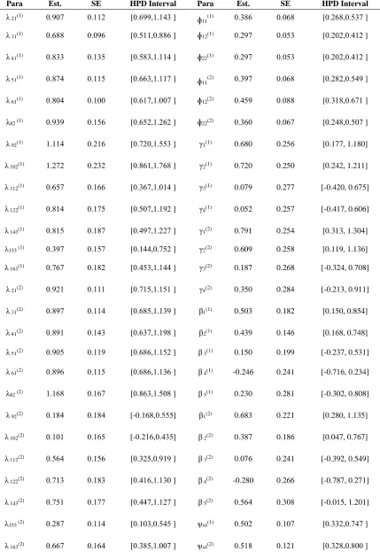
TABLE 1. Bayesian Estimation of Nonlinear LVMs with Mixed Variables under Prior I and II Using Censored Normal Distribution with Equal Spaces of Thresholds
Para Est. SE HPD Interval Para Est. SE HPD Interval
λ 21(1) 0.907 0.112 [0.699,1.143 ] ɸ11(1) 0.386 0.068 [0.268,0.537 ]
λ 31(1) 0.688 0.096 [0.511,0.886 ] ɸ12(1) 0.297 0.053 [0.202,0.412 ]
λ 41(1) 0.833 0.135 [0.583,1.114 ] ɸ22(1) 0.297 0.053 [0.202,0.412 ]
λ 51(1) 0.874 0.115 [0.663,1.117 ] ɸ11(2) 0.397 0.068 [0.282,0.549 ]
λ 61(1) 0.804 0.100 [0.617,1.007 ] ɸ12(2) 0.459 0.088 [0.318,0.671 ]
λ82 (1) 0.939 0.156 [0.652,1.262 ] ɸ22(2) 0.360 0.067 [0.248,0.507 ]
λ 92(1) 1.114 0.216 [0.720,1.553 ] γ1(1) 0.680 0.256 [0.177, 1.180]
λ 102(1) 1.272 0.232 [0.861,1.768 ] γ2(1) 0.720 0.250 [0.242, 1.211]
λ 112(1) 0.657 0.166 [0.367,1.014 ] γ3(1) 0.079 0.277 [-0.420, 0.675]
λ 122(1) 0.814 0.175 [0.507,1.192 ] γ4(1) 0.052 0.257 [-0.417, 0.606]
λ 143(1) 0.815 0.187 [0.497,1.227 ] γ1(2) 0.791 0.254 [0.313, 1.304]
λ153 (1) 0.397 0.157 [0.144,0.752 ] γ2(2) 0.609 0.258 [0.119, 1.136]
λ 163(1) 0.767 0.182 [0.453,1.144 ] γ3(2) 0.187 0.268 [-0.324, 0.708]
λ 21(2) 0.921 0.111 [0.715,1.151 ] γ4(2) 0.350 0.284 [-0.213, 0.911]
λ 31(2) 0.897 0.114 [0.685,1.139 ] β1(1) 0.503 0.182 [0.150, 0.854]
λ 41(2) 0.891 0.143 [0.637,1.198 ] β2(1) 0.439 0.146 [0.168, 0.748]
λ 51(2) 0.905 0.119 [0.686,1.152 ] β 3(1) 0.150 0.199 [-0.237, 0.531]
λ 61(2) 0.896 0.115 [0.686,1.136 ] β 4(1) -0.246 0.241 [-0.716, 0.234]
λ82 (2) 1.168 0.167 [0.863,1.508 ] β 5(1) 0.230 0.281 [-0.302, 0.808]
λ 92(2) 0.184 0.184 [-0.168,0.555] β1(2) 0.683 0.221 [0.280, 1.135]
λ 102(2) 0.101 0.165 [-0.216,0.435] β 2(2) 0.387 0.186 [0.047, 0.767]
λ 112(2) 0.564 0.156 [0.325,0.919 ] β 3(2) 0.076 0.241 [-0.392, 0.549]
λ 122(2) 0.713 0.183 [0.416,1.130 ] β 4(2) -0.280 0.266 [-0.787, 0.271]
λ 143(2) 0.751 0.177 [0.447,1.127 ] β 5(2) 0.564 0.308 [-0.015, 1.201]
λ153 (2) 0.287 0.114 [0.103,0.545 ] ψεδ(1) 0.502 0.107 [0.332,0.747 ]
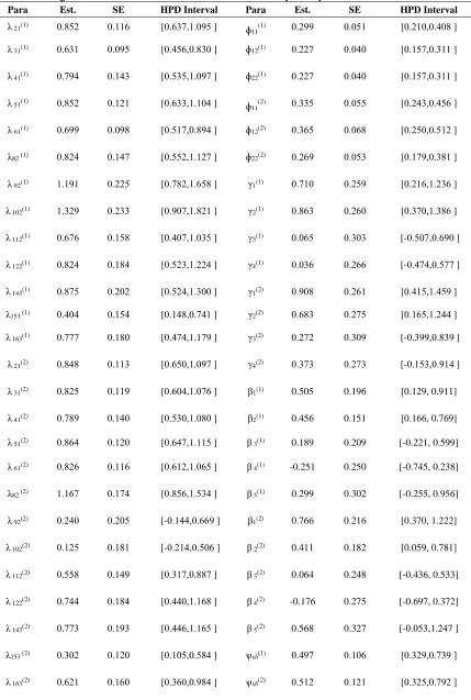
TABLE 2. Bayesian Estimation of Nonlinear LVMs with Mixed Variables under Prior I and II Using Censored Normal Distribution with Unequal Spaces of Thresholds
Para Est. SE HPD Interval Para Est. SE HPD Interval
λ 21(1) 0.852 0.116 [0.637,1.095 ] ɸ
11
(1) 0.299 0.051 [0.210,0.408 ]
λ 31(1) 0.631 0.095 [0.456,0.830 ] ɸ12(1) 0.227 0.040 [0.157,0.311 ]
λ 41(1) 0.794 0.143 [0.535,1.097 ] ɸ22(1) 0.227 0.040 [0.157,0.311 ]
λ 51(1) 0.852 0.121 [0.633,1.104 ] ɸ11(2) 0.335 0.055 [0.243,0.456 ]
λ 61(1) 0.699 0.098 [0.517,0.894 ] ɸ12(2) 0.365 0.068 [0.250,0.512 ]
λ82 (1) 0.824 0.147 [0.552,1.127 ] ɸ22(2) 0.269 0.053 [0.179,0.381 ]
λ 92(1) 1.191 0.225 [0.782,1.658 ] γ1(1) 0.710 0.259 [0.216,1.236 ]
λ 102(1) 1.329 0.233 [0.907,1.821 ] γ2(1) 0.863 0.260 [0.370,1.386 ]
λ 112(1) 0.676 0.158 [0.407,1.035 ] γ3(1) 0.065 0.303 [-0.507,0.690 ]
λ 122(1) 0.824 0.184 [0.523,1.224 ] γ4(1) 0.036 0.266 [-0.474,0.577 ]
λ 143(1) 0.875 0.202 [0.524,1.300 ] γ1(2) 0.908 0.261 [0.415,1.459 ]
λ153 (1) 0.404 0.154 [0.148,0.741 ] γ2(2) 0.683 0.275 [0.165,1.244 ]
λ 163(1) 0.777 0.180 [0.474,1.179 ] γ3(2) 0.272 0.309 [-0.399,0.839 ]
λ 21(2) 0.848 0.113 [0.650,1.097 ] γ4(2) 0.373 0.273 [-0.153,0.914 ]
λ 31(2) 0.825 0.119 [0.604,1.076 ] β1(1) 0.505 0.196 [0.129, 0.911]
λ 41(2) 0.789 0.140 [0.530,1.080 ] β2(1) 0.456 0.151 [0.166, 0.769]
λ 51(2) 0.864 0.120 [0.647,1.115 ] β 3(1) 0.189 0.209 [-0.221, 0.599]
λ 61(2) 0.826 0.116 [0.612,1.065 ] β 4(1) -0.251 0.250 [-0.745, 0.238]
λ82 (2) 1.167 0.174 [0.856,1.534 ] β 5(1) 0.299 0.302 [-0.255, 0.956]
λ 92(2) 0.240 0.205 [-0.144,0.669 ] β1(2) 0.766 0.216 [0.370, 1.222]
λ 102(2) 0.125 0.181 [-0.214,0.506 ] β 2(2) 0.411 0.182 [0.059, 0.781]
λ 112(2) 0.558 0.149 [0.317,0.887 ] β 3(2) 0.064 0.248 [-0.436, 0.533]
λ 122(2) 0.744 0.184 [0.440,1.168 ] β 4(2) -0.176 0.275 [-0.697, 0.372]
λ 143(2) 0.773 0.193 [0.446,1.165 ] β 5(2) 0.568 0.327 [-0.053,1.247 ]
λ153 (2) 0.302 0.120 [0.105,0.584 ] ψεδ(1) 0.497 0.106 [0.329,0.739 ]
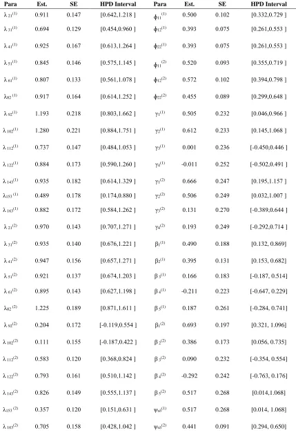
TABLE 3. Bayesian Estimation of Nonlinear LVMs with Mixed Variables under Prior I and II Using Truncated Normal Distribution with Equal Spaces of Thresholds
Para Est. SE HPD Interval Para Est. SE HPD Interval
λ 21(1) 0.911 0.147 [0.642,1.218 ] ɸ
11
(1) 0.500 0.102 [0.332,0.729 ]
λ 31(1) 0.694 0.129 [0.454,0.960 ] ɸ12(1) 0.393 0.075 [0.261,0.553 ]
λ 41(1) 0.925 0.167 [0.613,1.264 ] ɸ22(1) 0.393 0.075 [0.261,0.553 ]
λ 51(1) 0.845 0.146 [0.575,1.145 ] ɸ11(2) 0.520 0.093 [0.355,0.719 ]
λ 61(1) 0.807 0.133 [0.561,1.078 ] ɸ12(2) 0.572 0.102 [0.394,0.798 ]
λ82 (1) 0.917 0.164 [0.614,1.252 ] ɸ22(2) 0.455 0.089 [0.299,0.648 ]
λ 92(1) 1.193 0.218 [0.803,1.662 ] γ1(1) 0.505 0.232 [0.046,0.966 ]
λ 102(1) 1.280 0.221 [0.884,1.751 ] γ2(1) 0.612 0.233 [0.145,1.068 ]
λ 112(1) 0.737 0.147 [0.484,1.053 ] γ3(1) 0.001 0.236 [-0.450,0.446 ]
λ 122(1) 0.884 0.173 [0.590,1.260 ] γ4(1) -0.011 0.252 [-0.502,0.491 ]
λ 143(1) 0.935 0.182 [0.614,1.329 ] γ1(2) 0.666 0.247 [0.195,1.157 ]
λ153 (1) 0.489 0.178 [0.174,0.880 ] γ2(2) 0.506 0.249 [0.032,1.007 ]
λ 163(1) 0.882 0.172 [0.584,1.262 ] γ3(2) 0.131 0.270 [-0.389,0.644 ]
λ 21(2) 0.970 0.143 [0.707,1.271 ] γ4(2) 0.193 0.249 [-0.292,0.714 ]
λ 31(2) 0.935 0.140 [0.676,1.221 ] β1(1) 0.490 0.188 [0.132, 0.869]
λ 41(2) 0.947 0.156 [0.657,1.271 ] β2(1) 0.395 0.131 [0.153, 0.682]
λ 51(2) 0.921 0.137 [0.674,1.203 ] β 3(1) 0.166 0.183 [-0.187, 0.514]
λ 61(2) 0.895 0.143 [0.627,1.198 ] β 4(1) -0.211 0.223 [-0.647, 0.229]
λ82 (2) 1.225 0.189 [0.871,1.611 ] β 5(1) 0.187 0.261 [-0.284, 0.741]
λ 92(2) 0.204 0.172 [-0.119,0.554 ] β1(2) 0.693 0.197 [0.321, 1.096]
λ 102(2) 0.111 0.155 [-0.187,0.422 ] β 2(2) 0.386 0.173 [0.056, 0.735]
λ 112(2) 0.583 0.120 [0.368,0.824 ] β 3(2) 0.090 0.232 [-0.354, 0.554]
λ 122(2) 0.793 0.161 [0.510,1.142 ] β 4(2) -0.292 0.242 [-0.763, 0.176]
λ 143(2) 0.826 0.149 [0.555,1.137 ] β 5(2) 0.517 0.268 [0.014,1.068]
λ153 (2) 0.357 0.120 [0.151,0.631 ] ψεδ(1) 0.517 0.268 [0.014, 1.068]
TABLE 4. Bayesian Estimation of Nonlinear LVMs with Mixed Variables under Prior I and II Using Truncated Normal Distribution with Unequal Spaces of Thresholds
Para Est. SE HPD Interval Para Est. SE HPD Interval
λ 21(1) 0.852 0.155 [0.565,1.170 ] ɸ
11
(1) 0.432 0.095 [0.277,0.648 ]
λ 31(1) 0.655 0.139 [0.403,0.946 ] ɸ12(1) 0.322 0.068 [0.203,0.468 ]
λ 41(1) 0.894 0.174 [0.569,1.252 ] ɸ22(1) 0.322 0.068 [0.203,0.468 ]
λ 51(1) 0.802 0.151 [0.523,1.113 ] ɸ
11
(2) 0.445 0.086 [0.300,0.642 ]
λ 61(1) 0.762 0.141 [0.503,1.054 ] ɸ12(2) 0.507 0.108 [0.334,0.751 ]
λ82 (1) 0.896 0.178 [0.570,1.268 ] ɸ22(2) 0.370 0.086 [0.233,0.568 ]
λ 92(1) 1.278 0.234 [0.840,1.760 ] γ1(1) 0.570 0.247 [0.114,1.079 ]
λ 102(1) 1.322 0.232 [0.885,1.791 ] γ2(1) 0.662 0.240 [0.190,1.122 ]
λ 112(1) 0.756 0.151 [0.488,1.070 ] γ3(1) -0.029 0.250 [-0.495,0.477 ]
λ 122(1) 0.891 0.168 [0.599,1.250 ] γ4(1) 0.073 0.260 [-0.430,0.595 ]
λ 143(1) 0.940 0.187 [0.607,1.338 ] γ1(2) 0.744 0.243 [0.284,1.228 ]
λ153 (1) 0.466 0.163 [0.175,0.817 ] γ2(2) 0.517 0.253 [0.025,1.014 ]
λ 163(1) 0.907 0.185 [0.585,1.304 ] γ3(2) 0.205 0.257 [-0.285,0.746 ]
λ 21(2) 0.911 0.148 [0.639,1.219 ] γ4(2) 0.291 0.247 [-0.192,0.779 ]
λ 31(2) 0.872 0.147 [0.601,1.180 ] β1(1) 0.453 0.194 [0.081,0.855 ]
λ 41(2) 0.904 0.171 [0.592,1.258 ] β2(1) 0.428 0.140 [0.168,0.719 ]
λ 51(2) 0.875 0.151 [0.589,1.181 ] β 3(1) 0.168 0.202 [-0.224,0.571 ]
λ 61(2) 0.852 0.151 [0.577,1.170 ] β 4(1) -0.180 0.250 [-0.678,0.309 ]
λ82 (2) 1.210 0.195 [0.849,1.610 ] β 5(1) 0.299 0.299 [-0.232,0.911 ]
λ 92(2) 0.250 0.189 [-0.106,0.646 ] β1(2) 0.761 0.195 [0.398,1.163 ]
λ 102(2) 0.141 0.166 [-0.176,0.473 ] β 2(2) 0.376 0.182 [0.027,0.759 ]
λ 112(2) 0.604 0.130 [0.374,0.878 ] β 3(2) 0.073 0.244 [-0.406,0.569 ]
λ 122(2) 0.801 0.156 [0.525,1.136 ] β 4(2) -0.103 0.265 [-0.629,0.408 ]
λ 143(2) 0.874 0.164 [0.589,1.223 ] β 5(2) 0.448 0.286 [-0.073,1.037]
λ153 (2) 0.349 0.123 [0.142,0.629 ] ψεδ(1) 0.436 0.089 [0.294,0.638 ]
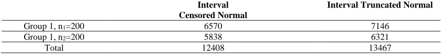
Table 5. Goodness of Fit Statistics (DIC) for LVMs with Mixed Variables and Equal Spaces of Thresholds under Prior I and II
Interval
Censored Normal Interval Truncated Normal
Group 1, n1=200 6583 7006
Group 1, n2=200 6088 6450
Total 12671 13456
Table 6. Goodness of Fit Statistics (DIC) for LVMs with Mixed Variables and Unequal Spaces of Thresholds under Prior I and II
Interval Censored Normal
Interval Truncated Normal
Group 1, n1=200 6570 7146
Group 1, n2=200 5838 6321
Total 12408 13467
The estimated multiple group nonlinear latent variable using censored normal distribution with equal spaces of thresholds is given by
𝜼𝒊(𝟏) = (𝟎. 𝟓𝟎𝟑)𝒙𝒊𝟏(𝟏)+ (𝟎.439)𝒙𝒊𝟐(𝟏)+ (𝟎.15𝟎)𝒙(𝟏)𝒊𝟏 𝒙𝒊𝟐(𝟏)+ (−𝟎.246)𝒙𝒊𝟏(𝟏)𝝃𝒊𝟐(𝟏)+ (𝟎.23𝟎)𝒙𝒊𝟏(𝟏)𝝃𝒊𝟏(𝟏)𝝃𝒊𝟐(𝟏)+ (𝟎.68𝟎)𝝃(𝟏)𝒊𝟏 + (𝟎.72𝟎)𝝃𝒊𝟐(𝟏)+ (𝟎. 𝟎79)𝝃𝒊𝟏(𝟏)𝝃𝒊𝟏(𝟏)+ (𝟎. 𝟎52)𝝃𝒊𝟐(𝟏)𝝃𝒊𝟐(𝟏)+ 𝜹𝒊(𝟏) (21)
𝜼𝒊(𝟐) = (𝟎.683)𝒙𝒊𝟏(𝟐)+ (𝟎.387)𝒙𝒊𝟐(𝟐)+ (𝟎. 𝟎76)𝒙(𝟐)𝒊𝟏 𝒙𝒊𝟐(𝟐)+ (−𝟎.28𝟎)𝒙𝒊𝟏(𝟐)𝝃𝒊𝟐(𝟐)+ (𝟎.564)𝒙𝒊𝟏(𝟐)𝝃𝒊𝟏(𝟐)𝝃𝒊𝟐(𝟐)+ (𝟎.791)𝝃(𝟐)𝒊𝟏 + (𝟎. 𝟔𝟎𝟗)𝝃𝒊𝟐(𝟐)+ (𝟎.187)𝝃𝒊𝟏(𝟐)𝝃𝒊𝟏(𝟐)+ (𝟎.35𝟎)𝝃𝒊𝟐(𝟐)𝝃𝒊𝟐(𝟐)+ 𝜹𝒊(𝟐) (22)
From the standard error estimates and the HPD intervals, we observe that all the linear effects of the covariates and the exogenous latent variables, and the interaction effects corresponding to 𝒙𝒊𝟏(𝟏)𝒙𝒊𝟐(𝟏), 𝒙𝒊𝟏(𝟏)𝝃𝒊𝟐(𝟏), 𝒙𝒊𝟏(𝟏)𝝃𝒊𝟏(𝟏)𝝃𝒊𝟐(𝟏) in the first group (Ohio) are quite
different from zero, 𝒙𝒊𝟏(𝟐)𝝃𝒊𝟐(𝟐), 𝒙𝒊𝟏(𝟐)𝝃𝒊𝟏(𝟐)𝝃𝒊𝟐(𝟐), 𝝃𝒊𝟏(𝟐)𝝃𝒊𝟏(𝟐), 𝝃𝒊𝟐(𝟐)𝝃𝒊𝟐(𝟐) in the second group (Kentucky) are quite different from zero, while the quadratic interaction effects corresponding to 𝜉𝑖1(1)𝜉𝑖1(1), 𝜉𝑖2(1)𝜉𝑖2(1) in first group (Ohio) and 𝒙𝒊𝟏(𝟐)𝒙𝒊𝟐(𝟐) in the second group (Kentucky) is small. Hence, the quadratic interaction causal effects of depression (𝜉𝑖1(1)𝜉𝑖1(1)), and also anxiety (𝜉𝑖2(1)𝜉𝑖2(1))in the first group (Ohio) and 𝒙𝒊𝟏(𝟐)𝒙𝒊𝟐(𝟐) in the second group (Kentucky) is not significant when given the other linear and interaction effects in the latent variable. As 𝜉𝑖1(1), 𝜉𝑖2(1), 𝑥𝑖1(1), 𝑥𝑖2(1) and 𝜉𝑖1(2), 𝜉𝑖2(2), 𝑥𝑖1(2), 𝑥𝑖2(2) in the first and second groups is related to the mixed ordered categorical and dichotomous variables, the
standard error estimate (0.241) and (0.281) correspond to 𝜷𝟒(𝟏) = (−𝟎.246), 𝜷𝟓(𝟏) =
(𝟎.23𝟎) is quite large, and the HPD interval, (-0.716, 0.234) and (-0.302, 0.808) is quite
wide. However, as 𝜷𝟒(𝟏) = (−𝟎.246), 𝜷𝟓(𝟏) = (𝟎.23𝟎) is quite different from zero in
magnitude. The standard error estimate (0.266), (0.308), (0.268) and (0.284) correspond to 𝜷𝟒(𝟐) = (−𝟎.28𝟎), 𝜷𝟓(𝟐) = (𝟎.564) and 𝜸𝟑(𝟐) = (𝟎.187), 𝜸𝟒(𝟐) = (𝟎.35𝟎) is quite large, and the HPD interval, (-0.787, 0.271), (-0.015, 1.201), (-0.324, 0.708) and (-0.213,
0.911) is quite wide. Hence the corresponding interaction effect is substantial.
𝜼𝒊(𝟏) = (𝟎. 𝟓𝟎𝟓)𝒙𝒊𝟏(𝟏)+ (𝟎.456)𝒙𝒊𝟐(𝟏)+ (𝟎.189)𝒙(𝟏)𝒊𝟏 𝒙𝒊𝟐(𝟏)+ (−𝟎.251)𝒙𝒊𝟏(𝟏)𝝃𝒊𝟐(𝟏)+ (𝟎.299)𝒙𝒊𝟏(𝟏)𝝃𝒊𝟏(𝟏)𝝃𝒊𝟐(𝟏)+ (𝟎.71𝟎)𝝃(𝟏)𝒊𝟏 + (𝟎.863)𝝃𝒊𝟐(𝟏)+ (𝟎. 𝟎65)𝝃𝒊𝟏(𝟏)𝝃𝒊𝟏(𝟏)+ (𝟎. 𝟎36)𝝃𝒊𝟐(𝟏)𝝃𝒊𝟐(𝟏)+ 𝜹𝒊(𝟏) (23)
𝜼𝒊(𝟐) = (𝟎.766)𝒙𝒊𝟏(𝟐)+ (𝟎.411)𝒙𝒊𝟐(𝟐)+ (𝟎. 𝟎64)𝒙(𝟐)𝒊𝟏 𝒙𝒊𝟐(𝟐)+ (−𝟎.176)𝒙𝒊𝟏(𝟐)𝝃𝒊𝟐(𝟐)+ (𝟎.568)𝒙𝒊𝟏(𝟐)𝝃𝒊𝟏(𝟐)𝝃𝒊𝟐(𝟐)+ (𝟎. 𝟗𝟎𝟖)𝝃(𝟐)𝒊𝟏 + (𝟎.683)𝝃𝒊𝟐(𝟐)+ (𝟎.272)𝝃𝒊𝟏(𝟐)𝝃𝒊𝟏(𝟐)+ (𝟎.373)𝝃𝒊𝟐(𝟐)𝝃𝒊𝟐(𝟐)+ 𝜹𝒊(𝟐) (24)
From the standard error estimates and the HPD intervals, we observe that all the linear effects of the covariates and the exogenous latent variables, and the interaction effects corresponding to 𝒙𝒊𝟏(𝟏)𝒙𝒊𝟐(𝟏), 𝒙𝒊𝟏(𝟏)𝝃𝒊𝟐(𝟏), 𝒙𝒊𝟏(𝟏)𝝃𝒊𝟏(𝟏)𝝃𝒊𝟐(𝟏) in the first group (Ohio) are quite
different from zero, 𝒙𝒊𝟏(𝟐)𝝃𝒊𝟐(𝟐), 𝒙𝒊𝟏(𝟐)𝝃𝒊𝟏(𝟐)𝝃𝒊𝟐(𝟐), 𝝃𝒊𝟏(𝟐)𝝃𝒊𝟏(𝟐), 𝝃𝒊𝟐(𝟐)𝝃𝒊𝟐(𝟐) in the second group (Kentucky) are quite different from zero, while the quadratic interaction effects corresponding to 𝜉𝑖1(1)𝜉𝑖1(1), 𝜉𝑖2(1)𝜉𝑖2(1) in first group (Ohio) and 𝒙𝒊𝟏(𝟐)𝒙𝒊𝟐(𝟐) in the second group (Kentucky) is small and not significant when given the other linear and interaction effects in the latent variable. As 𝜉𝑖1(1), 𝜉𝑖2(1), 𝑥𝑖1(1), 𝑥𝑖2(1) and 𝜉𝑖1(2), 𝜉𝑖2(2), 𝑥𝑖1(2), 𝑥𝑖2(2) in the first and second groups is related to the mixed ordered categorical and dichotomous variables, the
standard error estimate (0.209), (0.250), (0.302) correspond to 𝜷𝟑(𝟏) = (𝟎.189), 𝜷𝟒(𝟏) =
(−𝟎.251), 𝜷𝟓(𝟏) = (𝟎.299) is quite large, and the HPD interval, (-0.221, 0.599), (-0.745, 0.238) and (-0.255, 0.956) is quite wide. The standard error estimate (0.275), (0.327),
(0.309) and (0.273) correspond to 𝜷𝟒(𝟐) = (−𝟎.176), 𝜷𝟓(𝟐) = (𝟎.568) and 𝜸𝟑(𝟐) =
(𝟎.272), 𝜸𝟒(𝟐) = (𝟎.373) is quite large, and the HPD interval, (-0.697, 0.372), (-0.053,
1.247), (-0.399,0.839 and (-0.153,( 0.914 is quite wide. Hence the corresponding (
interaction effect is substantial.
The estimated multiple group nonlinear latent variable using truncated normal distribution with equal spaces of thresholds is given by
𝜼𝒊(𝟏) = (𝟎.49𝟎)𝒙𝒊𝟏(𝟏)+ (𝟎.395)𝒙𝒊𝟐(𝟏)+ (𝟎.166)𝒙(𝟏)𝒊𝟏 𝒙𝒊𝟐(𝟏)+ (−𝟎.211)𝒙𝒊𝟏(𝟏)𝝃𝒊𝟐(𝟏)+ (𝟎.187)𝒙𝒊𝟏(𝟏)𝝃𝒊𝟏(𝟏)𝝃𝒊𝟐(𝟏)+ (𝟎. 𝟓𝟎𝟓)𝝃(𝟏)𝒊𝟏 + (𝟎.612)𝝃𝒊𝟐(𝟏)+ (𝟎. 𝟎𝟎𝟏)𝝃𝒊𝟏(𝟏)𝝃𝒊𝟏(𝟏)+ (−𝟎. 𝟎11)𝝃𝒊𝟐(𝟏)𝝃𝒊𝟐(𝟏)+ 𝜹𝒊(𝟏) (25)
𝜼𝒊(𝟐) = (𝟎.693)𝒙𝒊𝟏(𝟐)+ (𝟎.386)𝒙𝒊𝟐(𝟐)+ (𝟎. 𝟎𝟗𝟎)𝒙(𝟐)𝒊𝟏 𝒙𝒊𝟐(𝟐)+ (−𝟎.292)𝒙𝒊𝟏(𝟐)𝝃𝒊𝟐(𝟐)+ (𝟎.517)𝒙𝒊𝟏(𝟐)𝝃𝒊𝟏(𝟐)𝝃𝒊𝟐(𝟐)+ (𝟎.666)𝝃(𝟐)𝒊𝟏 + (𝟎. 𝟓𝟎𝟔)𝝃𝒊𝟐(𝟐)+ (𝟎.131)𝝃𝒊𝟏(𝟐)𝝃𝒊𝟏(𝟐)+ (𝟎.193)𝝃𝒊𝟐(𝟐)𝝃𝒊𝟐(𝟐)+ 𝜹𝒊(𝟐) (26)
From the standard error estimates and the HPD intervals, we observe that all the linear effects of the covariates and the exogenous latent variables, and the interaction effects corresponding to 𝑥𝑖1(1)𝑥𝑖2(1), 𝑥𝑖1(1)𝜉𝑖2(1), 𝑥𝑖1(1)𝜉𝑖1(1)𝜉𝑖2(1) in the first group (Ohio) are quite
different from zero, 𝑥𝑖1(2)𝜉𝑖2(2), 𝑥𝑖1(2)𝜉𝑖1(2)𝜉𝑖2(2), 𝜉𝑖1(2)𝜉𝑖1(2), 𝜉𝑖2(2)𝜉𝑖2(2) in the second group (Kentucky) are quite different from zero, while the quadratic interaction effects corresponding to 𝜉𝑖1(1)𝜉𝑖1(1), 𝜉𝑖2(1)𝜉𝑖2(1) in first group (Ohio) and 𝑥𝑖1(2)𝑥𝑖2(2) in the second group (Kentucky) is small and not significant when given the other linear and interaction effects
in the latent variable.Hence the corresponding interaction effect is substantial.
𝜼𝒊(𝟏) = (𝟎.453)𝒙𝒊𝟏(𝟏)+ (𝟎.428)𝒙𝒊𝟐(𝟏)+ (𝟎.168)𝒙(𝟏)𝒊𝟏 𝒙𝒊𝟐(𝟏)+ (−𝟎.18𝟎)𝒙𝒊𝟏(𝟏)𝝃𝒊𝟐(𝟏)+ (𝟎.299)𝒙𝒊𝟏(𝟏)𝝃𝒊𝟏(𝟏)𝝃𝒊𝟐(𝟏)+ (𝟎.57𝟎)𝝃(𝟏)𝒊𝟏 + (𝟎.662)𝝃𝒊𝟐(𝟏)+ (−𝟎. 𝟎29)𝝃𝒊𝟏(𝟏)𝝃𝒊𝟏(𝟏)+ (𝟎. 𝟎73)𝝃𝒊𝟐(𝟏)𝝃𝒊𝟐(𝟏)+ 𝜹𝒊(𝟏) (27)
𝜼𝒊(𝟐) = (𝟎.761)𝒙𝒊𝟏(𝟐)+ (𝟎.376)𝒙𝒊𝟐(𝟐)+ (𝟎. 𝟎73)𝒙(𝟐)𝒊𝟏 𝒙𝒊𝟐(𝟐)+ (−𝟎. 𝟏𝟎𝟑)𝒙𝒊𝟏(𝟐)𝝃𝒊𝟐(𝟐)+ (𝟎.448)𝒙𝒊𝟏(𝟐)𝝃𝒊𝟏(𝟐)𝝃𝒊𝟐(𝟐)+ (𝟎.744)𝝃(𝟐)𝒊𝟏 + (𝟎.517)𝝃𝒊𝟐(𝟐)+ (𝟎. 𝟐𝟎𝟓)𝝃𝒊𝟏(𝟐)𝝃𝒊𝟏(𝟐)+ (𝟎.291)𝝃𝒊𝟐(𝟐)𝝃𝒊𝟐(𝟐)+ 𝜹𝒊(𝟐) (28)
From the standard error estimates and the HPD intervals, we observe that all the linear effects of the covariates and the exogenous latent variables, and the interaction effects corresponding to 𝑥𝑖1(1)𝑥𝑖2(1), 𝑥𝑖1(1)𝜉𝑖2(1), 𝑥𝑖1(1)𝜉𝑖1(1)𝜉𝑖2(1) in the first group (Ohio) are quite
different from zero, 𝑥𝑖1(2)𝜉𝑖2(2), 𝑥𝑖1(2)𝜉𝑖1(2)𝜉𝑖2(2), 𝜉𝑖1(2)𝜉𝑖1(2), 𝜉𝑖2(2)𝜉𝑖2(2) in the second group (Kentucky) are quite different from zero, while the quadratic interaction effects corresponding to 𝜉𝑖1(1)𝜉𝑖1(1), 𝜉𝑖2(1)𝜉𝑖2(1) in first group (Ohio) and 𝑥𝑖1(2)𝑥𝑖2(2) in the second group (Kentucky) is small and not significant when given the other linear and interaction effects
in the latent variable. Hence the corresponding interaction effect is substantial.
The results corresponding to the first and second groups and ordered categorical variables and covariates with hidden continuous normal distribution (censored normal distribution) for variables and hidden continuous normal distribution (truncated normal distribution with known parameters) as well as two types of thresholds (with equal and unequal distances for categories) are reported in Tables (1:2). We noticed that the SE values are small values in the first and second groups.
The results corresponding to the first and second groups and ordered categorical variables and covariates with hidden continuous normal distribution (truncated normal distribution with known parameters) for variables and hidden continuous normal distribution (truncated normal distribution with known parameters) as well as two types of thresholds (with equal and unequal spaces for categories) are reported in Tables (3:4). We observed that the SE values are small values in the first and second groups.
The highest posterior density (HPD) of all the parameters was calculated. We noticed that the effectiveness of the HPD intervals is convenient for ordered categorical variables when using censored normal distribution, truncated normal distribution.
To reveal the effectiveness of DIC for model comparison, we reanalysed the data sets via
a nonlinear latent variable model with interaction term in the latent variable model (M4).
The DIC values obtained were compared to those obtained under the correct model. The
results are presented in Tables (5:6).
The DIC values of censored normal distribution, truncated normal distribution with equal spaces of thresholds, are (12671) and (13456) respectively.
The model fitting DIC of LVMs with mixed data using censored normal distribution and is less than the model fitting DIC of LVMs with mixed data truncated normal distribution. However, it performs very well for the mixed variables with censored normal distribution.
The DIC values of censored normal distribution, truncated normal distribution with unequal spaces of thresholds, are (12408) and (13467) respectively.
The best fitted model with a smallest DIC value is a censored normal distribution with unequal spaces of thresholds (12408). Also, the DIC value of truncated normal distribution with equal spaces of thresholds is (13456). As a result, we observed that the performance of DIC is not satisfactory and would be worse with mixed data using truncated normal distribution with unequal spaces of thresholds.
7. Conclusions and Recommendations
The multi-sample nonlinear models which involving nonlinear effects with nonlinear covariates and latent variables are very common in social and behavioural sciences. The first purpose of this analysis was to use multi-sample nonlinear LVMs with nonlinear covariates and latent variables to obtain all the estimated parameters. The second purpose is to solve the problem of mixed variables by using hidden continuous normal distribution (censored normal distribution and truncated normal distribution) and to solve the problem of mixed ordered categorical and dichotomous covariates using hidden continuous normal distribution (truncated normal distribution with known parameters). The proposed procedures have been done using two types of thresholds (with equal and unequal categories distances). However, this assumption is likely to be violated in many practical applications.
In this paper, a Bayesian approach is proposed for analysing multi-sample nonlinear models with mixed variables. In addition to point estimation, we provide statistical methods to obtain standard deviations estimates, and model comparison using the Deviance Information Criterion (DIC) owing to the complexity of the proposed model. As we have seen, difficulties arising from the nonlinear causal relationships among the latent variables and the discrete nature of mixed data manifest variables are alleviated by data augmentation with some MCMC methods. This strategy is very powerful and can be applied to other more complex models.
References
1. Akaike, H. (1973). Information theory and an extension of the maximum
likelihood principle. Proceedings of the 1973 Second international symposium on information theory, 267-281.
2. Booth, B. M., Leukefeld, C., Falck, R., Wang, J. and Carlson, R. (2006).
Correlates of rural methamphetamine and cocaine users: Results from a multistate community study. Journal of Studies on Alcohol and Drugs, 67(4), 493.
3. Broemeling, L. D. (1985). Bayesian analysis of linear models: Dekker New York.
4. Cai, J.-H., Song, X.-Y. and Lee, S.-Y. (2008). Bayesian analysis of non-linear
structural equation models with mixed continuous, ordered and unordered categorical, and non-ignorable missing data. Statistics and its Interface, 1, 99-114.
5. Geman, S. and Geman, D. (1984). Stochastic relaxation,Gibbs distribution,and the
Bayesian restoration of images. IEEE Transactions on Pattern Analysis and Machine Intelligence, (6), 721-741.
6. Geyer, C. J. (1992). Practical markov chain monte carlo. Statistical Science,
473-483.
7. Lee, S.Y. (2007). Structural Equation Modeling: A Bayesian Approach.