Bayesian Analysis of Linear and Nonlinear Latent Variable Models with Fixed Covariate and Ordered Categorical Data

with Fixed Covariate and Ordered Categorical Data

Thanoon Y. Thanoon

Department of Mathematical Science, Faculty of Science Universiti Teknologi Malaysia, 81310, Skudai, Johor, Malaysia

Department of Operation Management Technique, Technical College of Management, Northern Technical University, Mosul, Iraq

[email protected]

Robiah Adnan

Department of Mathematical Science, Faculty of Science Universiti Teknologi Malaysia, 81310, Skudai, Johor, Malaysia [email protected]

Abstract

In this paper, ordered categorical variables are used to compare between linear with covariate and nonlinear interactions of covariates and latent variables in Bayesian structural equation models. Gibbs sampling method is applied for estimation and model comparison. Hidden continuous normal distribution (censored normal distribution) is used to handle the problem of ordered categorical data. Statistical inferences, which involve estimation of parameters and their standard deviations, and residuals analyses for testing the selected model, are discussed. The proposed procedure is illustrated by a real data. Analyses are done by using OpenBUGS program.

Keywords: Structural equation models, Bayesian analysis, latent variables, Gibbs sampling, ordered categorical data.

1. Introduction

Structural equation modeling (SEM) is a statistical approach to testing hypotheses about the relationships among observed and latent variables. Observed variables also called indicator variables or manifest variables. Latent variables also denoted as unobserved variables or factors. Examples of latent variables in education are math ability and intelligence and in psychology are depression and self confidence. The latent variables cannot be measured directly. Researchers must define the latent variable in terms of observed variables (Khine, 2013).

At present, most statistical theory and computer software in the field of SEMs are based on models that involve only linear relationships among the manifest and the latent variables. More statistically sound methods for linear and nonlinear SEMs and factor analysis have been proposed by Lee and Song (2003),Lee and Song (2005),Lee (2006) ,

equation models to nonlinear models that include nonlinear terms of the latent variables is obvious. Practically, nonlinear relationships such as quadratic and interaction terms among the variables are important in establishing the substantive theory in many areas. The rapid growth of SEMs is due to the demand of subtle models and the related statistical methods for solving complex research problems in various fields.

The main objective of this paper is to propose a Bayesian approach for analysing linear and nonlinear SEMs with ordered categorical variables. The Deviance Information Criterion (DIC; see Spiegelhalter et al., 2002) will be used for model comparison.

The main idea is to handle the ordered categorical variables in the Bayesian analysis and to treat the underlying latent continuous measurements as hypothetical missing data and augment them with the observed data in the posterior analysis.

The paper is organized as follows. Model Description is described in section 2. Bayesian estimation of structural equation models which contain Linear and nonlinear models are described in Section 3. Models comparison using (DIC) are described Section 4. A case study is presented in section 5. Empirical results, which are obtained from a case study, are discussed in Section 6. Some concluding remarks are given in section 7.

2. Model Description

Consider the following measurement equation for a p1 manifest random vector y_i

1,..., n,

i i i

y    w  i  (1)

where (p1) is the vector of intercepts,  (p q) is the factor loading matrix,

( 1)

i

w q is a latent random vector and _i(p1) is a random vector of error measurements with distribution N[0, _], _ is diagonal andiis independent with wi.

We let i(q11) and i(q21) be latent subvectors of wi, and consider the following

structural equation:

( , )

i i F xi i i

       (2)

Where (q₁q₁) and (q₁q₂) are matrices of regression coefficients, _i and _i are independently distributed as N[0,] and N[0,_], where _ is a diagonal covariance matrix. It is assumed that     _{0 q1} is a nonzero constant that is independent with elements in_. x_i (x_i1)T is a vector of covariate.

Let Y (y₁,...,y_n) is underlying latent continuous measurements are unobservable. The information associated with y is given by an observable ordered categorical vector

1

( ,..., _n)

1 1

1

1, 1 1, 1

1

, s 1 , s

z z

s s z s z

y

z

z

if

z

y



















 





 



 









 





 





(3)

Where for k 1,..., ,s z_k is an integral value in {0,1,...,b_k} and

1

,0 ,1 ... ,_k ,_k

k k k b k b

     _ . In general, we set

1

,0 , ,_k

k k b

   _  , For the kth variable, there are b_k1 categories which are defined by the unknown thresholds_{k j,} . The integral values {0,1,...,b_k} of z_k are just used for specifying the categories that contain the corresponding elements in y_k (Lee, 2007).

It has been pointed out by Lee et al. (1990) that single-sample models with ordered categorical variables are not identified without imposing identification conditions. This is also the case for multi-sample models. To solve this problem, we use the common method (see, for example, Lee et al., 1995; Shi and Lee, 1998) of fixing some thresholds at preassigned values. For convenience, we assume that the positions of the fixed elements are the same for each group.

3. Bayesian estimation of structural Equation models

The objective of this section is to describe a Bayesian approach for analyzing the preceding nonlinear structural equation models in the context of ordered categorical data. Nice features of a Bayesian approach include the following: (a) Prior knowledge can be directly incorporated in the analysis. As a result, more accurate parameter estimates can be obtained under situations with good prior information; (b) As mentioned by many articles on Bayesian analysis of structural equation models (Lee, 2006; Lee and Shi, 2000; Lee et al., 2010; Lee et al., 2007; Song and Lee, 2002, 2004; Song et al., 2011; Yang and Dunson, 2010), the sampling-based Bayesian methods do not rely on asymptotic theory; and (c) The Bayesian estimates and the ML estimates have the same optimal asymptotic properties.

We will utilize the useful strategy of data augmentation described in the Bayesian

estimation of SEMs with ordered categorical variables. Let Z ( ,...,z₁ z_n) be the

ordered categorical data matrix, and let Y (y₁,...,y_n) and  (w₁,...,w_n) be the matrices of latent continuous measurements and latent variables, respectively. The

observed data [Z] is augmented with the latent data [Y,] in the posterior analysis. The

joint Bayesian estimates of _. To describe the Bayesian approach for the proposed

nonlinear structural equation model, letZ { ,...,z₁ z_n} be the observed data set of ordered categorical variables, and  be vector that contains the unknown free parameters under the model M.

In a Bayesian approach,  is considered random with a prior distribution and a prior density function, say p( ) . Bayesian inference is based on the observed data Z and

( )

Let p Z( , ) be the joint probability density function of Z and  under model M. Based on a basics in probability,p Z( , )  p(Z | ) ( ) p  , where p(Z | ) and p( | Z) are conditional density functions; it follows that

log p( | Z) log p(Z | ) log ( )  p  ₍₄₎

The function p( | Z) is called the posterior density function of the unknown parameters. In Equation (4) the posterior density function p( | Z) depends on likelihood function

(Z | )

p  and prior distribution p( ) _{. The function} p(Z | ) depends on the sample size, whereas p( ) does not. For large samples, the prior of  plays a less important role, and the posterior density function p( | Z) is close to the likelihood function p( ) . Thus, the Bayesian and ML approaches are asymptotically equivalent, and the Bayesian estimates have the same optimal asymptotical properties as the ML estimates. However, p( ) plays a significant role in the Bayesian approach in the situations where the sample size is small, or the information given by ordered categorical data Z.

In this article, we define the Bayesian estimate of  as the mean of the posterior distribution (called the posterior mean). For simple structural equation models, the posterior mean can be obtained through direct integration. However, due to the complexity of the proposed nonlinear structural equation model with covariates and dichotomous variables, the relating integral does not have a closed form. We apply some MCMC methods in statistical computing to solve this problem. Let yibe the unobserved

variables that correspond to the manifest ordinal variables in zi , and let Y (y1,...,yn)

and  (w1,...,wn). If we can draw a sufficiently large number of observations ( ) ( ) ( )

{(t ,t ,Y t );t 1,..., }T from the joint posterior distribution ( ,p  ,Y | Z), then the Bayesian estimate of  and the standard error estimates can be obtained from the following sample mean and sample variance matrix, respectively:

^

1 ( ) 1 ( ) ( )

1 1

, var( | ) ( 1) ( )( ) .

T T

t t t

t t

T Z T

        

 









It is necessary to specify the prior distributions for components in  when deriving the conditional distribution of  given (,Y Z, ) in Step a. In general Bayesian analyses, the conjugate prior distributions have been found to be flexible and convenient (Broemeling, 1985).

This kind of prior distribution has been widely applied to many Bayesian analyses in structural equation models (Lee and Song, 2004 ; Song and Lee, 2007). Hence, the following well-known conjugate prior distributions are used:

0 0 0 0 0 0

1 1

0 0 0 0

( ) [ , ], ( ) [ , ], ( | ) [ , ],

( ) [ , ], ( ) [ , ]

k k k k k k k k

q k k k

p N H p N H p N H

p W R p Gamma

     



       

   

 

  

Where _k is the kth diagonal element of ,k and k are the kth rows of  and



 , respectively. H_0 diag(₀₁2,...,₀2_p), and  ₀, _0k, _0k,   _0k, _0k, ₀, _0k,H H₀, _0k,

andR₀are assumed to be given by the prior information. In general, prior information can be obtained from causal observation or theoretical consideration of experts, or the analyses of past data. As pointed out by Kass and Raftery (1995) , priors are often picked for convenience when there is a lack of accurate prior knowledge, because the effect of the priors in Bayesian estimation is small when the sample size is fairly large. For completeness, the conditional posterior distributions of ,Y and the components of based on the conjugate prior distributions. These results are useful for writing the computer program to implement the Gibbs sampler.

In the Bayesian approach, we need to evaluate the posterior distribution [ , ,   Z]. This distribution is rather complicated. To capture its characteristics, we will try to draw a sufficiently large number of observations from it such that the empirical distribution of the generated observations is a close approximation to the true distribution. A good candidate for simulating observations from the posterior distribution is the Gibbs sampler (Geman and Geman, 1984), which iteratively simulates  , and  from the full conditional distributions. However, owing to the presence of the ordered categorical variables, these conditional distributions are rather complicated to derive and simulating observations from them is difficult. This motivates the further augmentation of the latent matrix Yin the posterior analysis, and the consideration of the joint posterior distribution

[ , , ,  Y Z]. To implement the Gibbs sampler for generating observations of this

posterior distribution, we start with initial starting values ( (0), (0),(0),Y (0)) , then simulate ( (1), (1),(1),Y (1)) and so on according to the following procedure. At the mth iteration with current values (m),(m),(m),Y (m)

1. Generate (m1)from ( ) ( ) ( )

( m , m , m , Z)

p   Y

2. Generate (m1) fromp( (m1),(m),Y (m), Z)

3. Generate ((m1),Y (m1)) from ( 1) ( 1)

( , m , m , Z)

p  Y     (7)

The cycle defined above generates ( 1) ( 1)

( , m , m , Z)

p  Y     after the mth iteration. As m

approaches infinity, the joint distribution of ((m),(m),(m),Y (m))can be shown to approach the joint posterior distribution[ , , ,  Y Z]. (see Geman and Geman, (1984); Geyer, (1992((.

simulated from the joint posterior distribution will be used to calculate the Bayesian estimates and other related statistics.

4. Model Comparisons

A model comparison statistic that takes into account the number of unknown parameters in the model is the DIC (see Spiegelhalter et al., 2002). This statistic is intended as a generalization of the Akaike Information Criterion (AIC; Akaike, (1973) . Under a competing model M_k with a vector of unknown parameters _k of dimensiond_k, let

( )

{kt :t 1,..., }T be a sample of observations simulated from the posterior distribution.

The DIC for M_kis computed as follows:

( )

1 2

log ( | , ) 2 ,

T

t

k k k k

t

DIC p Z M d

T  

 



(8)

In model comparison, the model with the smaller DIC value is selected. As mentioned in Spiegehalter et al. (2003), practical applications of DIC, it is important to note the followings:

(a) If the difference in DIC is small, for example less than 5, and the models make very different inferences, then just reporting the model with the lowest DIC could be misleading. (b) DIC can be applied to non-nested models. (c) Similar to the Bayes factor (Kass and Raftery, 1995) BIC, and AIC, DIC gives a clear conclusion to support the null hypothesis or the alternative hypothesis.

To illustrate the use of DIC for model comparison, we analyzed the same data by a linear and a nonlinear structural equation model with the same measurement model:

1*x(i,1) 1 1 2 2 3 3 ,

i i i i i

        

(9)

1 2 2 3 3 4 2 2 5 1 2 1 1

2 2 3 3 4 2 2

*x(i,1)+ *x(i,1)* + *x(i,1)* + *x(i,1)* + *x(i,1)* +

+ +

i i i i i i i i

i i i i i

             

       



 

(10)

The DIC value corresponding to the linear and nonlinear structural equation model produced by OpenBUGS. The correct nonlinear structural equation model is selected.

5. Case Study and Example

satisfied’). The sample size of the whole data set is extremely large. To illustrate the Bayesian methods, we only analyze a synthetic data set with sample size n = 200.

Our Bayesian linear & nonlinear SEMs defined in Equation (9) and Equation (10) respectively. Hence, some quadratic and interaction effects of the latent variables are considered. To illustrate the Bayesian methods in analyzing linear and nonlinear structural equation models with ordered categorical variables, we use a real data set that is related to random vectors z_i (z_1i,z_2i,...,z_11i), let y_i (y_1i,y_2i,...,y_11i) be the latent continuous random vector corresponds to the ordinal variables z_1i,z_2i,...,z_11i

wherez_i,i 1,..., n are ordered categorical variables that are related with 4 latent variables

1 2 3

( , , , )

i i i i i

w      ,_i ( _i1, _i2,...,_i11), with the following values of the parameters in

1 2 11

( , ,..., )

     and  ( ₁, ₂,...,₁₁ )

11 12 13

21 22 23

31 32 33

_{  } 

 

     

_{  } 

  (11)

The relationships of the latent variables in wi ( ,  i _{1 , 2i}i )are assessed by the nonlinear

structural equation which is described in Equation (10). A covariate x (200*1) and those corresponding to 1,2 and 3 are 0 30,

1 0

R 8, respectively. The following accurate prior inputs of the hyperparameter values in the conjugate prior distributions of the parameters are considered:

Prior I. Elements in ₀,_0k and _0k in Equation (6) are set equal to the following values and initial values are equal to 1;

Prior I. Elements in ₀,_0k and _0k in Equation (6) are set equal to the true values;

1

0 8

R  , H0u,H0k and H0k are taken to be 0.25 times the identity matrices;

0k 10

  , _0k 8, ₀ 30.

The prior is informative and can have a significant effect on the parameter estimates for a small sample size case.

6. Results and Discussion

The objective of this section is to present results of a case study to reveal the empirical performances of the Bayesian estimates and the DIC for model comparison.

For linear and nonlinear SEMs, we have the following proposed models:

1 1 1 2 2 3 3

1 1 1 2 2 3 3 4 1 2

1 1 1 2 2 3 3 4 1 3

1 1 1 2 2 3 3 4 2 3

1: *x(i,1) ,

2 : *x(i,1) ,

3 : *x(i,1) ,

4 : *x(i,1) ,

5 :

i i i i i

i i i i i i i

i i i i i i i

i i i i i i i

i Model Model Model Model Model

        

                                   



    

     

     

     

1 2 2 3 3 4 2 2

5 1 2 1 1 2 2 3 3 4 2 2

*x(i,1)+ *x(i,1)* + *x(i,1)* + *x(i,1)* +

*x(i,1)* + + +

i i i i

i i i i i i i i

       

            



  (12)

In this paper, a Bayesian approach is introduced for analysing linear and nonlinear SEMs with ordered categorical variables. The Bayesian estimates of the unknown parameters and the Bayesian model selection statistic DIC are obtained using recently developed powerful tools in statistical computing. All the computational work can be accomplished via the recently developed and freely available software OpenBUGS. Therefore, our proposed method can be conveniently applied on real data. The purpose of this analysis is to compare between linear and nonlinear Bayesian SEMs with ordered categorical data. There are some limitations of the current analysis. First, due to the design of questionnaires and the nature of the problems in behavioral, educational, medical and social sciences, data are often in ordered categorical variables with observations in discrete form. In analyzing ordered categorical data, the basic assumption in SEM is that the data comes from a continuous normal distribution which is clearly violated, and rigorous analysis that takes into account the ordered categorical nature is necessary.

Hence, Clearly, routinely treating ordered categorical variables as normal may lead to erroneous conclusions (see Lee et al., 1990; Olsson, 1979).

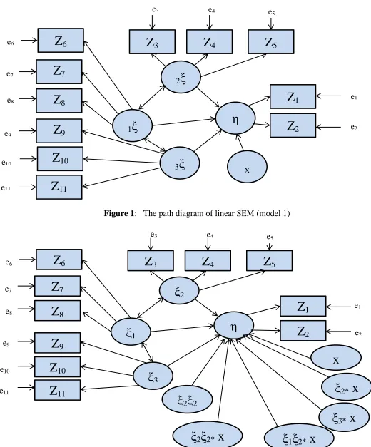
Figure 1: The path diagram of linear SEM (model 1)

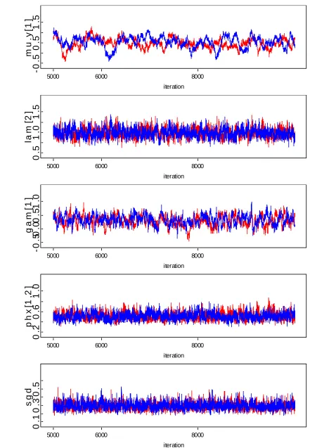
Figure 2. The path diagram of nonlinear SEM (model 5). e9

e10

Z

Z

Z

e4 e3

e1

e2 e8

e7

η

Z

Z

2

ξ

Z

Z

Z

1

ξ

Z

Z

Z

e6

e5

3

ξ

e11

X

ξ

x

x

e9

e10

Z

Z

Z

e4 e3

e1

e2 e8

e7

η

Z

2

Z

ξ

Z

Z

Z

ξ

Z

Z

Z

e6

e5

ξ

e11

ξ

ξ

x

ξ

ξ

ξ

x

iteration

5000 6000 8000

m

u

.y

[1

]

-1

.0

0

.0

1

.0

iteration

5000 6000 8000

la

m

[2

]

0

.5

1

.0

1

.5

iteration

5000 6000 8000

g

a

m

[1

]

-0

.5

0

.5

1

.5

iteration

5000 6000 8000

p

h

x

[1

,2

]

0

.2

0

.6

1

.0

iteration

5000 6000 8000

s

g

d

0

.1

0

.3

0

.5

iteration

5000 6000 8000

m

u

.y

[1

]

-0

.5

0

.5

1

.5

iteration

5000 6000 8000

la

m

[2

]

0

.5

1

.0

1

.5

iteration

5000 6000 8000

g

a

m

[1

]

-0

.5

0

.0

0

.5

1

.0

iteration

5000 6000 8000

p

h

x

[1

,2

]

0

.2

0

.6

1

.0

iteration

5000 6000 8000

s

g

d

0

.1

0

.3

0

.5

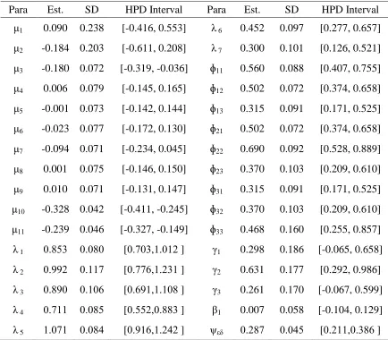
Table 1. Bayesian Estimation of nonlinear SEM with Ordered Categorical Variables

Para Est. SD HPD Interval Para Est. SD HPD Interval

μ1

0.504 0.261 [-0.083,0.975] ɸ12 015.0 01070 [01380,01669 ]

μ2

0.161 0.222 [-0.318,0.555] ɸ13 01307 01089 [01.70,015.8 ]

μ3

-0.097 0.072 [-0.236,0.044] ɸ21 015.0 01070 [01380,01669 ]

μ4

0.089 0.081 [-0.065,0.253] ɸ22 01683 0109. [01507,01880 ]

μ5

0.074 0.073 [-0.071,0.219] ɸ23 01370 01098 [01003,01580 ]

μ6

0.067 0.081 [-0.090,0.229] ɸ31 01307 01089 [01.70,015.8 ]

μ7

-0.021 0.075 [-0.168,0.125] ɸ32 01370 01098 [01003,01580 ]

μ8

0.099 0.080 [-0.060,0.256] ɸ33 01077 01.06 [01009,01808 ]

μ9

0.101 0.076 [-0.052,0.249] γ1 0.314 0.190 [-0.072, 0.665]

μ10

-0.298 0.043 [-0.384,-0.212] γ2 0.449 0.362 [-0.270, 1.153]

μ11

-0.216 0.047 [-0.307,-0.123] γ3 0.416 0.408 [-0.320, 1.259]

λ 1 _{01836 0108.}

[01689,.1005] γ4 0.067 0.277 [-0.433, 0.633]

λ 2 _{01988 01..3}

[01783,.1006] β1 -0.076 0.064 [-0.191, 0.064]

λ 3 _{01880 01.05}

[01687,.1.00] β2 0.060 0.083 [-0.101, 0.224]

λ 4 _{017.8 01087}

[01555,01895] β3 -0.042 0.101 [-0.245, 0.152]

λ 5 _{.1086 0108.}

[0193.,.1050] β4 -0.006 0.076 [-0.176, 0.135]

λ6 _{01050 01097}

[01087,01660] β5 0.001 0.069 [-0.133, 0.144]

λ 7 _{01097 01.03 [01.03,01530]} ψεδ _{0.292 0.046 [0.215, 0.392]}

ɸ11 _{01580 01089}

Table 2. Bayesian Estimation of linear SEM with Ordered Categorical Variables

Table 3. The DIC Values for Linear and Nonlinear EMs with Ordered Categorical Variables and Covariates

The results corresponding to the nonlinear SEM with covariates under Type I and II inputs, and ordered categorical variables are reported in Table (1). We observed that the SD values are very small in the nonlinear SEM.

The results corresponding to the linear SEM and covariate under Type I and II inputs, and ordered categorical variables are reported in Table (2). We observed that the SD values are very small in the linear SEM with covariate.

Linear with covariates Nonlinear with covariates

5011.0 5034.0

Para Est. SD HPD Interval Para Est. SD HPD Interval

μ1 0.090 0.238 [-0.416, 0.553] λ 6 0.452 0.097 [0.277, 0.657]

μ2 -0.184 0.203 [-0.611, 0.208] λ 7 0.300 0.101 [0.126, 0.521]

μ3 -0.180 0.072 [-0.319, -0.036] ɸ11 0.560 0.088 [0.407, 0.755]

μ4 0.006 0.079 [-0.145, 0.165] ɸ12 0.502 0.072 [0.374, 0.658]

μ5 -0.001 0.073 [-0.142, 0.144] ɸ13 0.315 0.091 [0.171, 0.525]

μ6 -0.023 0.077 [-0.172, 0.130] ɸ21 0.502 0.072 [0.374, 0.658]

μ7 -0.094 0.071 [-0.234, 0.045] ɸ22 0.690 0.092 [0.528, 0.889]

μ8 0.001 0.075 [-0.146, 0.150] ɸ23 0.370 0.103 [0.209, 0.610]

μ9 0.010 0.071 [-0.131, 0.147] ɸ31 0.315 0.091 [0.171, 0.525]

μ10 -0.328 0.042 [-0.411, -0.245] ɸ32 0.370 0.103 [0.209, 0.610]

μ11 -0.239 0.046 [-0.327, -0.149] ɸ33 0.468 0.160 [0.255, 0.857]

λ 1 01853 01080 [01703,.10.0 ] γ1 0.298 0.186 [-0.065, 0.658]

λ 2 01990 01..7 [01776,.103. ] γ2 0.631 0.177 [0.292, 0.986]

λ 3 01890 01.06 [0169.,.1.08 ] γ3 0.261 0.170 [-0.067, 0.599]

λ 4 017.. 01085 [01550,01883 ] β1 0.007 0.058 [-0.104, 0.129]

The results corresponding to the linear and nonlinear SEM with covariates under Type I and II inputs, we observed that the SD values in linear SEM are smaller than the SD values for the nonlinear SEM with covariates. However, it is expected that the empirical performance would be worse with the nonlinear SEM with covariates.

The HPD intervals of all the parameters were computed. We observed that the performances of the HPD intervals in linear SEM and covariate are satisfactory for ordered categorical variables. To reveal the performance of DIC for model comparison, we reanalysed the data sets via a nonlinear SEM and covariate in the structural equation (Model 5). The DIC values obtained were compared to those obtained under the correct model. Results are presented in Table 3.

The model fitting DIC in linear SEM is less than the DIC value in nonlinear SEM in the ordered categorical variables. As a result, we observed the performance of DIC is not satisfactory and would be worse under nonlinear effect and ordered categorical variables. However, it performs very well with linear effect with covariate and ordered categorical variables.

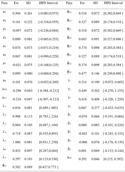
Convergence of the Gibbs sampler are monitored by the plots of several simulated sequences of the individual parameters with different starting values and are presented in Figures 3 and 4 respectively. Bayesian estimates were obtained from T=10000 iterations after discarding 5000 burn-in iterations in linear and nonlinear SEMs with covariates.

7. Conclusions and Recommendations

References

1. Akaike, H. (1973). Information Theory and an Extension of the Maximum Likelihood Principle. Proceedings of the 1973 Second international symposium on information theory, 267-2811

2. Broemeling, L. D. (1985). Bayesian Analysis of Linear Models: Dekker New York.

3. Bollen, K. A. and Paxton, P. (1998). Interactions of latent variables in structural equation models. Structural Equation Modeling, 5, 267-293 1

4. Cai, J.-H., Song, X.-Y. and Lee, S.-Y. (2008). Bayesian Analysis of Nonlinear Structural Equation Models with Mixed Continuous, Ordered and Unordered Categorical, and Nonignorable Missing Data. Statistics and its Interface, 1, 99-114.

5. Geman, S. and Geman, D. (1984). Stochastic Relaxation,Gibbs Distribution,and the Bayesian Restoration of Images. IEEE Transactions on Pattern Analysis and Machine Intelligence, (6), 721-741.

6. Geyer, C. J. (1992). Practical Markov Chain Monte Carlo. Statistical Science, 473-483 1

7. Kass, R. E. and Raftery, A. E. (1995). Bayes Factors. Journal of the American Statistical Association, 90, 773–795.

8. Khine, M. S. (2013). Application of Structural Equation Modeling in Educational Research and Practice: Springer1

9. Lee, S.-Y., Poon, W.-Y. and Bentler, P. M. (1995). A Two‐Stage Estimation of Structural Equation Models with Continuous and Polytomous Variables. British Journal of Mathematical and Statistical Psychology, 48(2), 339-358.

10. Lee, S.-Y. and Song, X.-Y. (2005). Maximum Likelihood Analysis of a Two-Level Nonlinear Structural Equation Model with Fixed Covariates. Journal of Educational and Behavioral Statistics, 30(1), 1-26. doi: 10.3102/10769986030001026

11. Lee, S.-Y., Song, X.-Y., Cai, J. H., So, W. Y., Ma, C. W. and Chan, C. N. (2009). Nonlinear Structural Equation Models with Correlated Continuous and Discrete

Data. Br J Math Stat Psychol, 62(Pt 2), 327-347. doi:

10.1348/000711008X292343

12. Lee, S.-Y. and Song, X.-Y. (2003). Model Comparison of Nonlinear Structural Equation Models with Fixed Covariates. PSYCHOMETRIK, 68(1), 27-47.

13. Lee, S.-Y. and Song, X.-Y. (2004). Evaluation of the Bayesian and Maximum Likelihood Approaches in Analyzing Structural Equation Models with Small Sample Sizes. Multivariate Behavioral Research, 39(4), 653-686.

14. Lee, S.-Y., Song, X.-Y. and Tang, N.-S. (2007). Bayesian Methods for Analyzing Structural Equation Models with Covariates, Interaction, and Quadratic Latent Variables. Structural Equation Modeling: A Multidisciplinary Journal, 14(3), 404-434. doi: 10.1080/10705510701301511.

15. Lee, S.-Y. and Song, X.-Y. (2012). Basic and Advanced Structural Equation Models for Medical and Behavioural Sciences. Hoboken: Wiley.

17. Lee, S.-Y., Song, X.-Y. and Cai, J.-H. (2010). A Bayesian Approach for Nonlinear Structural Equation Models with Dichotomous Variables using Logit and Probit Links. Structural Equation Modeling, 17(2), 280-302.

18. Lee, S. and Tang, N. (2006). Analysis of Nonlinear Structural Equation Models with Nonignorable Missing Covariates and ordered categorical data. Statistica Sinica, 16(4), 1117.

19. Lu, B., Song, X.-Y. and Li, X.-D. (2012). Bayesian Analysis of Multi-Group Nonlinear Structural Equation Models with Application to Behavioral Finance.

Quantitative Finance, 12(3), 477-488. doi: 10.1080/14697680903369500

20. Lee, S.-Y. (2006). Bayesian Analysis of Nonlinear Structural Equation Models with Nonignorable Missing Data. Psychometrika, 71(3), 541-564. doi: 10.1007/s11336-006-1177-1

21. Lee, S.-Y. and Shi, J.-Q. (2000). Bayesian Analysis of Structural Equation Model With Fixed Covariates. Structural Equation Modeling: A Multidisciplinary Journal, 7(3), 411-430. doi: 10.1207/s15328007sem0703_3

22. Lee, X.-Y. S. a. S.-Y. (2002). A Bayesian Approach for Multigroup Nonlinear Factor Analysis. Structural Equation Modeling, 9(4), 523–553 1

23. Lee, X.-Y. S 1a. S.-Y. (2004). Bayesian Analysis of Two-Level Nonlinear Structural Equation Models With Continuous and Polytomous Data. British Journal of Mathematical and Statistical Psychology, 57, 29–52 1

24. Lee, S.-Y., Poon, W.-Y. and Bentler, P. (1990). Full Maximum Likelihood Analysis of Structural Equation Models with Polytomous Variables. Statistics & probability letters, 9(1), 91-97.

25. Power, M., Bullingen, M. and Hazper, A. (1999) The World Health Organization WHOQOL-100: Tests of the universality of quality of life in 15 different cultural groups worldwide. Health Psychology, 18, 495–505.

26. Rubin, D. B. (1991). EM and beyond. Psychometrika, 56(2), 241-254 1

27. Schumacker, R. E. and Marcoulides, G. A. (1998). Interaction and Nonlinear Effects in Structural Equation Modeling: Lawrence Erlbaum Associates Publishers1

28. Song, X. Y., & Lee, S. Y. (2007). Bayesian Analysis of Latent Variable Models with Nonignorable Missing Outcomes from Exponential Family. Statistics in Medicine, 26, 681–693.

29. Song, X.-Y., Lu, Z.-H., Hser, Y.-I. and Lee, S.-Y. (2011). A Bayesian Approach for Analyzing Longitudinal Structural Equation Models. Structural Equation Modeling: A Multidisciplinary Journal, 18(2), 183-194. doi: 10.1080/10705511.2011.557331.

30. Shi, J.-Q. and Lee, S.-Y. (1998). Bayesian Sampling-Based Approach for Factor Analysis Model with Continuous and Polytomous Data. British Journal of Mathematical and Statistical Psychology, 51, 233-252.

31. Spiegelhalter, D. J., Best, N. G., Carlin, B. P., & van der Linde, A. (2002). Bayesian Measures of Model Complexity and Fit (with Discussion). Journal of the Royal Statistical Society, Series B, 64(4), 583-639 1