http://www.sciencepublishinggroup.com/j/ijtam doi: 10.11648/j.ijtam.20180401.11
ISSN: 2575-5072 (Print); ISSN: 2575-5080 (Online)
Mathematical Model and a Case Study for Multi-Commodity
Transportation Problem
Niluka Rodrigo
1, *, Lashika Rjapaksha
2Department of Mathematics, University of Peradeniya, Peradeniya, Sri Lanka
Email address:
[email protected] (N. Rodrigo), [email protected] (L. Rjapaksha) *Corresponding author
To cite this article:
Niluka Rodrigo, Lashika Rjapaksha. Mathematical Model and a Case Study for Multi-Commodity Transportation Problem. International Journal of Theoretical and Applied Mathematics. Vol. 4, No. 1, 2018, pp. 1-7. doi: 10.11648/j.ijtam.20180401.11
Received: October 31, 2017; Accepted: December 18, 2017; Published: January 15, 2018
Abstract:
The problem of locating distribution centers is one of the most important issues in design of supply chain. The design of the distribution system is an important issue for almost every company. Wide range of problems arising in practical applications can be formulated as Mixed-integer nonlinear Models. Multi-commodity distribution system design is a generalization of a facility location problem where we have several commodities, and shipment from a plant to customer occurs through a distribution center. This report presents a real life distribution problem. The problem is to determine which distribution centers to use so that all customer demands are satisfied, production capacities are not exceeded, and the total distribution cost that is the fixed cost of operating the distribution center and the transportation cost is minimized. A computer program (Software R) is developed to obtain the optimal solution.Keywords:
Transportation Problem, Multi-Commodity Distribution, Mixed-Integer Nonlinear Programs, Software R1. Introduction
Today, global marketing and manufacturing is developing rapidly. With this rapid development, competition among
manufacturing companies becomes more severe.
Manufacturing products, shipping products into warehouses and delivering products to customers is very difficult today. Therefore every company is looking for a logistic system to balance the overall supply chain of the company.
Deciding locations of distribution centers are the most difficult part in supply chain management because inefficient locations will result in excess cost. Thus management should recognize the future conditions when making facility location decisions. Multi-commodity distribution system design is a generalization of a facility location problem where we have several commodities, and shipment from plant to customer occurs through a distribution center.
One of the most important attempts was taken by Geoffrion_et al [1] in which a mixed integer programming model was formulated for the multi-commodity location problem. Distribution center locations, capacities of the distribution centers, customers, and transportation flow
patterns for all commodities were determined Solution to the
problem was presented based on Benders Decomposition
Method. It is possible to solve problem with any number of commodities from this decomposition method. The transportation part of the problem was broken into a separate classical transportation problem for each commodity. The major conclusion obtained from this study is the effectiveness of the Benders Decomposition as a computational strategy for multi-commodity distribution location problem.
Simple and effective Genetic Algorithm has been presented by Fernandes et al [2] for the two stage capacitated
facility location problem, which arises in freight
other one is based on rounding linear relaxations of the problem. Computational experiments were performed to set the best Genetic Algorithm parameters to ensure the quality of the solutions.
Lelkes et_al [3] has developed a new model by
considering much simpler problem where several
commodities produced in several plants, distributed to several destination sites according to the customer demands.
The model was developed for multi-commodity
transportation and supply chain problem which is expressed as a step-wise constant function. From this study, new model is tested on multi-commodity transportation problem of SAB Miller Europe and compared with the other methods from the literature. Also feasibility checking method has been developed for large scale mixed integer linear programming problem having binary variables in the objective function.
In addition to the above studies, Afshari et al [4] has
presented a multi-objective mixed integer linear
programming formulation for location within network distribution problem. To formulate this model, some assumptions were considered; two potential central warehouses that at least one of them should be located, limited capacities for both central and regional warehouses, transportation cost per unit is a coefficient of the distance between the central and the regional warehouses, and between the regional warehouses and the customers respectively and the minimum level of the customer satisfaction. Two Objectives have been considered; minimizing the total cost including establishment of warehouses and the transportation cost, and maximizing the customer satisfaction. In this case study, Afshari has get data from Automotive Part Distribution Corporation and solved the formulated model using Lingo Software package.
Also, Agarwal et al [5] has provided with an integrated model to minimize total transportation cost by determining the optimal locations, flows, shipment composition, and shipment cycle time. A Model has formulated for a two tier
distribution network. Agarwal has made following
assumptions to formulate the mathematical model; each distribution receives the goods only from the warehouses or directly from plants, the average monthly demand at various nodes has been taken as independent of each other, manufacturing location always has the material ready when the order arrives, major safety stock is maintained at the warehouses for its direct sale and for the distributors which are replenished at regular intervals by the warehouse. But the operating cost at each warehouse is not considered.
Uzorh et al [6] has developed a linear programming method problem to solve the cost related problem. The objective of the formulated problem was to minimize the total transportation cost and to increase the profit on sale. A case study has done to apply the linear programming method to real world problem. TORA software has used to solve the problem. Sensitivity analysis has done to classify the optimal solution and check the allowable increase and decrease of the cost coefficient and r.h.s values of constraints.
Linderstorm [7] restricted the survey to the standard linear
multi-commodity minimum cost network flow where all the constraints and the costs are linear functions. Multi-commodity minimum cost flow problem has converted into a maximum flow by setting all supply and demands to zero, and adding artificial arc going from each sink to
corresponding source. Price-directive decomposition,
Resource-directive decomposition, partitioning methods is given as the most common three categories to solve the multi-commodity minimum cost flow problem.
Jil et al [8] has presented a mathematical model for two stages planning of transportation and inventory for several products. A local manufacturing company in which the total supply exceeds the total demand is considered for the survey. The rational unit cost is a new concept that has been used to develop the mathematical model. The objective of this study was to plan both transportation and inventory for both stages. Behmardi et al [9] has presented a dynamic multi-period multi-commodity capacitated facility location problem in supply chain to maximize net-profit during the planning horizon. Only one-echelon supply chain has considered. Once fictitious plants are opened it cannot be closed, moving capacity between existing plants is not allowed and expansion or reduction of existing plants is allowed are some of the assumptions made to simplify the model. Mixed integer programming formulation has been modeled by ILOG Optimization Programming Language (OPL) studio 3.5. Five different types of test problems include different number of customers’ commodities and plants have been considered.
Also, H. Afshari et al [10] have presented a multi-objective mixed integer programming formulation for location within network distribution problem. Objectives are to minimize the total cost including establishment and transportation cost and to maximize the customer satisfaction. The problem describes two location layers in single period. We determine the volume of the inventory in both stocks and middle warehouses.
2. Materials and Methods
Transportation problem is an important area in operations research. The objective is to determine the amount that should be transported from each source to each destination, so that the total transportation cost is minimized. It consists with a linear objective function and linear constraints.
converted into balanced by adding a dummy demand or a dummy supply.
2.1. Solution Procedure of Balanced Transportation Problem
Transportation problem can be solved using two stages; determining initial basic feasible solution and then determine the optimal solution.
There are three standard methods to find an initial basic feasible solution:
1. Northwest corner rule
2. Minimum cost method
3. Vogel’s approximation method/Regret method
Optimal solution can be find using Stepping stone method and Modified Distribution Method or U-V Method.
2.2. Multi-Commodity Transportation Problem
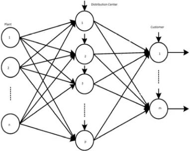
Multi-commodity transportation problem is a problem where several commodities, shipped from a plant to a customer occur through a distribution center. The objective of the multi commodity transportation problem is to determine which distribution centers to use so that all customer demands are satisfied, production capacities are not exceeded, and the total distribution cost, that is, the fixed cost of operating the distribution centers and the transportation cost, is minimized.
2.3. Mathematical Model of Multi-Commodity Transportation Problem
Figure 1. A Multi-commodity DistributionNetwork.
Objective function of the multi-commodity transportation problem consists with three parts; minimizing the total distribution cost, the annual operating cost and the cost of flow through the distribution centers.
1.Total distribution cost is the cost of producing and shipping i th commodity from j thplant to lth customer via
kth distribution center.
i.e.
q n p m
i jk l i jk l i 1 j 1 k 1 l 1
c x
= = = =
∑∑∑∑
(1)Where,
cijkl: Unit cost of producing and shipping ith commodity
from jth plant to customer via kth distribution center.
: Amount of ith commodity shipped from jth plant to customer l via kth distribution center.
2.Annual operating cost can be defined as follows:
p k k k 1
f z
=
∑
(2)Where,
fk: Fixed annual operating cost of the kth distribution center.
{
thk 1 ; if k distribution center is open
z
0; otherwise
Here, the operating cost is added only if kth the distribution center is open. So zk is a binary variable.
3.The cost of flow through the distribution center can be defined as follows:
If kth distribution center serves to the lth customer and if the demand of ith commodity to lth customer is given by Dil,
i.e
p q m
k i l kl k 1 i 1 l 1
v D y
= = =
∑∑∑
(3)Where,
Dil: Demand of ith commodity by lth customer
vk: Unit cost of flow through the kth distribution center
{
th thk l 1 ; if k distribution center surves l customer
y
0; otherwise
=
Total transportation cost can be calculated by adding above three equations:
i.e.
q n p m p i jk l i jk l k k i 1 j 1 k 1 l 1 k 1
c x f z
= = = = =
+
∑∑∑∑
∑
+
p q m
k i l kl k 1 i 1 l 1
v D y
= = =
∑∑∑
Following requirements should be satisfied to reach to the objective function:
a) Number of units of ith commodity that can be
transported from j th plant to lth customer through the kth
distribution cannot exceed the supply of each commodity.
i.e.
p m
i jk l ij k 1 l 1
x S for all i, j.
= =
≤
∑∑
Where,
: Number of amount of ith commodity shipped from jth
plant to lthcustomer via kth distribution center.
Sij: Production capacity of ith commodity at jth plant. b) Number of amounts of ith commodity shipped from jth
plant to lth customer via kth distribution center must be equal to the amount of that ith commodity produced at all plants that is designed for that the customer and shipped via that distribution center. This constraint
forces to take the value 0, if =0. That is
whenever =0, lth customer is not served by kth
distribution center.
i.e
n
i jk l i l k l j 1
x D y for all i, k, l =
=
∑
c) Each customer is served by only one distribution
center.
i.e
p kl k 1
y 1 for all l
=
=
∑
d) Flow through kth distribution center, if open (that is
= 1) is between the lower bound and the upper
bound . That ensure the logical relationship between
the y and z variables; that is = 1 if and only if =1 for some l.
i.e
(
)
q m
k k i l k l k k i 1 l 1
L z D y U z k 1,..., p
= =
≤
∑ ∑
≤ =Where,
Lk,, Uk: Minimum and maximum allowable annual flow through thekth distribution center.
e) Amount of commodity shipped to customer via
distribution center cannot be negative.
i.e xi jk l ≥ 0 ∀i, j, k, l
is a binary variable. =1 if customer is served by the
distribution center k.
i.e
y
k l≥
0 or 1
∀
k, l
f) is also a binary variable. If = 1, kth distribution center is opened on that site and if = 0, there is no a distribution center.
i.e
z
k≥
0 or 1
∀ =
k 1,..., p
Formulated mathematical model for multi-commodity transportation problem:
q n p m p i jk l i jk l k k i 1 j 1 k 1 l 1 k 1
Minimize c x f z
= = = = =
=
∑∑∑∑
+∑
+ p q m
k i l kl k 1 i 1 l 1
v D y
= = =
∑∑∑
Subject to,
p m
i jk l ij k 1 l 1
x
S
for all i, j.
= =
≤
∑∑
n
i jk l i l k l j 1
x D y for all i, k, l = =
∑
p kl k 1y 1 for all l
=
=
∑
(
)
q m
k k i l k l k k i 1 l 1
L z D y U z k 1,..., p
= =
i jk l
x
≥
0
∀
i, j, k, l
3. Results
3.1. Case Study
The problem arises in a local company categorized under
Candy and Confectionery-Manufacturers Equipment.
Company has only one plant. Chocolate toffees, wafers biscuit, extruded snacks and many more products are
produced in this plant. This problem involves the
transportation of a truckload of their products from a plant to seven distribution centers, and to 15 customers at a minimum transportation cost in Sri Lanka.
Required cost, capacities and demands of distribution centers to commodity are given in following tables 1 to 7.
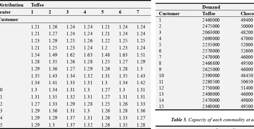
Table 1. Unit cost (in Rupees) of producing and shipping toffees to each customer through each distribution center.
Distribution Toffee
center 1 2 3 4 5 6 7
Customer
1 1.21 1.26 1.24 1.24 1.21 1.24 1.24
2 1.21 1.27 1.24 1.24 1.21 1.24 1.24
3 1.23 1.29 1.25 1.26 1.22 1.25 1.25
4 1.21 1.25 1.23 1.24 1.2 1.23 1.24
5 1.54 1.49 1.62 1.63 1.48 1.63 1.51
6 1.28 1.35 1.26 1.28 1.25 1.27 1.29
7 1.29 1.36 1.27 1.29 1.26 1.28 1.3
8 1.35 1.43 1.34 1.32 1.31 1.35 1.43
9 1.34 1.41 1.33 1.31 1.3 1.34 1.42
10 1.3 1.34 1.31 1.3 1.27 1.3 1.31
11 1.31 1.35 1.32 1.31 1.27 1.31 1.31
12 1.27 1.33 1.29 1.28 1.25 1.26 1.33
13 1.29 1.36 1.31 1.3 1.26 1.28 1.36
14 1.29 1.29 1.37 1.31 1.26 1.33 1.27
15 1.29 1.3 1.37 1.32 1.26 1.35 1.28
Table 2. Unit cost (in Rupees) or producing and shipping Chocolates to each customer through each distribution center.
Distribution Chocolate
center 1 2 3 4 5 6 7
Customer
1 27.66 30.28 28.83 29.19 27.37 28.83 28.83
2 27.77 30.46 28.85 29.26 27.34 28.85 28.95
3 27.92 30.51 29.04 29.49 27.43 29.12 29.09
4 28.17 30.42 29.27 29.78 27.49 29.32 29.37
5 41.21 39.25 44.68 45.37 38.91 45.37 40.29
6 30.95 34.19 30.08 30.99 29.62 30.54 31.17
7 31.84 35.76 30.93 31.97 30.28 31.45 32.36
8 34.39 38.39 33.79 32.89 32.33 34.39 38.39
9 35.23 39.41 34.58 33.67 32.89 35.31 39.93
10 31.99 33.73 32.24 31.82 30.39 31.82 32.24
11 31.62 33.71 32.05 31.69 30.15 31.62 31.65
12 31.13 34.05 31.78 31.48 29.85 30.27 33.93
13 31.97 35.23 32.76 32.49 30.41 31.14 35.26
14 31.42 31.69 35.42 32.41 29.88 33.73 30.31
15 31.41 31.92 35.22 32.82 29.91 34.27 30.64
Table 3. Unit cost (in Rupees) of producing and shipping Biscuit to each customer through each distribution center.
Distribution Biscuit packet
center 1 2 3 4 5 6 7
customer
1 26.79 28.54 27.57 27.81 26.6 27.57 27.57
2 26.89 28.69 27.61 27.89 26.6 27.61 27.68
3 26.82 28.4 27.5 27.78 26.51 27.55 27.53
4 26.89 28.21 27.54 27.84 26.49 27.57 27.6
5 36.48 35.09 38.92 39.41 34.85 39.41 35.83
6 29.29 31.62 28.67 29.32 28.34 28.99 29.45
7 29.22 31.62 28.66 29.3 28.26 28.98 29.54
8 30.91 33.42 30.53 29.97 29.62 30.91 33.42
9 31.42 34.03 31.01 30.44 29.95 31.47 34.36
10 29.65 30.8 29.81 29.53 28.58 29.53 29.81
11 29.29 30.64 29.57 29.34 28.35 29.29 29.31
12 29.3 31.34 29.76 29.55 28.4 28.7 31.26
13 29.6 31.74 30.11 29.94 28.57 29.05 31.76
14 29.43 29.61 32.18 30.11 28.37 31.02 28.67
15 29.47 29.82 32.11 30.45 28.43 31.46 28.93
Table 4. Demand for each commodity by the customer.
Demand
Customer Toffee Chocolate Biscuit
1 2460000 49400 74190
2 2475000 50000 74286
3 2063000 48200 78571
4 2690000 47000 80000
5 2235000 52000 73571
6 2570000 52600 73207
7 2470000 46000 75000
8 2466800 49500 78929
9 2625000 46000 73571
10 2390000 48450 73214
11 2280500 50650 78500
12 2750000 51400 73571
13 2400000 46000 70064
14 2470000 49800 72500
15 2360000 49500 71286
Table 5. Capacity of each commodity at each distribution center.
Distribution Center Commodity
Toffee Chocolate Biscuit
1 10000000 200000 310000
2 2500000 58000 75000
3 5500000 102000 166000
4 5500000 100000 160428
5 5200000 110000 160000
6 5300000 100000 150000
7 5000000 110000 150000
Table 6. Fixed cost (in Rupees) at each distribution center and per unit cost of flow through the distribution center.
Distribution
Center Toffee Chocolate Biscuit Fixed cost
1 0.516 0.78 0.54 3470870
2 0.78 0.78 0.552 2654949
3 0.576 0.576 7.26 3921083
4 4.86 4.86 5.22 5772084
5 4.98 4.98 4.62 4952241
6 7.26 7.26 7.26 4043158
Table 7. Capacity of each plant for each commodity.
Commodity Plant
1 39000000
2 780000
3 1171428
3.2. Optimum Transportation Schedule
Formulate model in chapter 2 can be solved with respect to the data gathered from the company and to satisfy the company requirements. It is solved using software environment R to determine the optimum transportation schedule so that the total transportation cost will be minimized and optimum solution to the problem given in table 8.
Table 8. Optimum transportation schedule.
Commodity Distribution center Customer Total cost (Rs) Cost of flow through the distribution center (Rs)
Toffee 1 1 2982000 11193100
Toffee 1 2 3006600 11225440
Toffee 5 6 3221234 25924315
Toffee 5 9 3405034 26382015
Chocolate 1 4 2151200 9155340
Chocolate 1 8 2439950 9443254
Biscuit 5 4 2118834 12392915
Biscuit 5 8 2337984 12607117
Total minimum Cost =Rs.1183223496.00
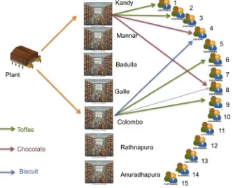
Figure 2. Graphical representation of the optimal transportation schedule.
4. Discussion
Solving the above transportation problem using R software package, Minimum transportation cost is Rs.1183223496.00. The amount, Rs. 1195599652.00 represents the minimum annually transportation cost for the company to transport its products from the plant to seven customers via two distribution centers. So clearly we can see that the optimum solution we obtained through our process is more profitable than the existing one. It is also clear from the result that to minimize the transportation cost chocolates can be transported only through the Kandy distribution center, and
biscuits can be transported only via Colombo distribution center. Figure 2 illustrates the graphical representation of the optimal transportation schedule to distribute each commodity to customers via two distribution centers.
5. Conclusion
transportation cost. It is clear from the result and the given data, to minimize the transportation cost only two distribution centers can be used. Also only few customer demands were satisfied. By increasing the capacity or reducing the transportation cost, company can select dealers in a more profitable way to satisfy more customers’ demands.
References
[1] A. M. Geoffrion, G. W. Graves "Multi-commodity Distribution System Design by Benders Decomposition", Management Science, Vol. 20, No. 5, Theory Series, Mathematical Programming (Jan., 1974), 822-844.
[2] Diogo R. M. Fernandes, Caroline Rocha, Daniel Aloise, Glaydston M. Ribeiro, Enilson M. Santos, Allyson SilvaA "Simple and effective genetic algorithm for the two-stage capacitated facility location problem", Computers & Industrial Engineering 75 (2014) 200–208, www.elsevier.com/ locate/caie
[3] Zoltan Lelkes, Endre Rev, Tivadar Farkas, Zsolt Fonyo, Tibor Kovacs and Ian Jones "Multi-commodity transportation and supply problem with stepwise constant cost function", European Symposium on Computer Arded Process Engineering – 15 L. Puigjaner and A. Espuña (Editors) © 2005 Elsevier Science.
[4] H. Afshari, M. Amin-Nayeri, A. A. Jaafari "A Multi-objective Approach for Multi-commodity Location within Distribution
Network Design Problem", Proceeding of the International Multiconference of Engineers and Computer Scientists 2010 Vol III, IMECS 2010.
[5] Gopal Agarwal and Lokesh Vijayvargy "Designing of Multi-Commodity, Multi Location Integrated Model for Effective Logistics Management", Proceeding of the International Multi conference of Engineers and Computer Scientists 2011 Vol II, IMECS 2011.
[6] Engr. Dr. Uzorh, A. C1and Nanna Innocent "Supply Chain Management Optimization Problem " The International Journal Of Engineering And Science (IJES) || Volume || 3 || Issue || 6 || Pages || 01-09 || 2014 || ISSN (e): 2319 – 1813 ISSN (p): 2319–1805.
[7] Joe Lindstrom "Multi-commodity Network Flow - Methods and Applications", [email protected].
[8] P. Ji1, K. J. Chen, and Q. P. Yan "A Mathematical Model for a Multi-Commodity, Two-Stage Transportation and Inventory Problem" International Journal of Industrial Engineering, 15(3), 278-285, 2008.
[9] Behrouz Behmardi and Shiwoo Lee "Dynamic Multi-commodity Capacitated Facility Location Problem in Supply Chain", Proceedings of the 2008 Industrial Engineering Research Conference J. Fowler and S. Mason, eds.