1959
PREDICTION OF OSTEOARTHRITIS USING LINIER
VECTOR QUANTIZATION BASED TEXTURE FEATURE
1LILIK ANIFAH, 2MAURIDHI HERY PURNOMO, 3TATI L R MENGKO
1 Informatics Department, Faculty of Engineering, Universitas Negeri Surabaya, Kampus Unesa Ketintang
Jl. Ketintang, Surabaya East Java 60231, Indonesia
2 Electrical Engineering Department, Institut Teknologi Sepuluh Nopember, Surabaya, Kampus ITS Keputih Sukolilo Surabaya East
Java 60111, Indonesia
3 Electrical Engineering Department, Institut Teknologi Bandung, Jl. Ganesha 10/12 -Bandung, West Java, Indonesia
E-mail: 1[email protected]
ABSTRACT
Osteoarthritis estimated as the eighth-leading nonfatal burden of disease in the world is the one important reason why it is investigated. The status of osteoarthritis is important because it is used as a basis for determining treatment for patients. The aim of this research is analyzing the texture feature of Junction Space Area (JSA) and design system based texture feature in order to predict the severity of osteoarthritis in the knee using a linear vector quantization. Textures extracted in this study are first order, second order, and gray level run length matrix. Several stages involved as the research procedures covering image processing, feature extraction, learning process, and testing process. The result of feature extraction obtained several FO, GLCM and GLRLM features for each cluster with overlapping conditions, making it difficult to classify using linear methods, so learning used linear vector quantization (LVQ). Feature extraction was carried out for both training data and testing data. The training process, which was divided into several stages namely first order learning, GLCM learning data, GLRLM learning data, and combined learning data features. learning process for the aforementioned features of combined learning data used learning parameter rate of 0.5 with epoch values of 1000, 5000, 10000, and 15000. The best results obtained when using a system using LVQ based on GLCM features. But the disadvantage of this system is that it cannot recognize grade 2 well where recognizing grade 2.
Keywords: Osteoarthritis, FO, GLCM, GLRLM, LVQ
1. INTRODUCTION
Osteoarthritis (OA) is a disorder characterized by loss of articular cartilage, bone hypertrophy at the margin, subchondral sclerosis and various biochemistry and changes in morphology of synovial membranes and joint capsule [1]. The severity of osteoarthritis is expressed as grade 0 to grade 4, grade 0 is normal and grade 4 is the worst condition [2]-[4].
Some of the reasons why osteoarthritis is important to study are because the number of osteoarthritis patients is high. Osteoarthritis estimated as the eighth-leading nonfatal burden of disease in the world [5]. Another reason is osteoarthritis cannot be cured, what can be done is how to improve the quality of life of patients [6].
Classification of osteoarthritis based on x-ray image has been carried out by several researchers throughout the world, research based on Junction
Space Area (JSA) features or texture-based images. Research that used image processing are segmentation of Junction Space Area (JSA) using active shape model [7], gabor filter based morphology [8], and other methods [9-13].
In [8] and [9] based on the Junction Space Area feature, where [8] discussed about Junction Space Area segmentation using morphological processes and [9] detected the severity of osteoarthritis using the fisher score. Classification using Self Organizing Map (SOM) GLCM-based which was previously used by gabor kernel and CLAHE for the preprocessing [10]. In [11] also based on texture feature with different parameters. However, both researchers [10-11] still discuss classification methods in partial texture-based. So it is needed to investigate the osteoarthritis severity prediction based on texture feature and its combination.
1960 predict the severity of osteoarthritis in the knee using a linear vector quantization. Textures extracted in this study are first order, second order, and gray level run length matrix.
2. METHODOLOGY 2.1 Data
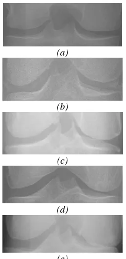
[image:2.612.359.488.125.390.2]This study used x-ray images of knees as the data obtained from Osteoarthritis Initiative (OAI). The method for conducting an x-ray approached to fixed-flexion PA view (see Figure 1). Moreover, Figure 2, which also became one of data that would be processed in this study, portrayed an example of KL-Grade 0 to KL-Grade 4. The data, further, were classified into two categories namely data for learning and testing. The total data for learning category were five for each KL-Grade and 499 data were for testing category.
Figure 1. The method for conducting an x-ray approached to fixed-flexion PA view [14]
2.2 Methods
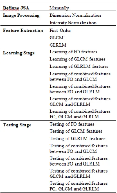
This study used semiautomatic method, in which determining Junction Space Area (JSA) was still conducted by the users manually. The defined JSA was then put into classifications to reveal the level of severity automatically based on the calculated texture information.
There were several stages involved as the research procedures covering image processing, feature extraction, learning process, and testing process. Image processing was conducted to put the images into different clusters. The process included dimensional normalization, grayscale, intensity normalization processes using CLAHE. Afterwards, the results of CLAHE process were treated in feature extraction process to extract the features of First Order, Gray Level Co-occurrence Matrix (GLCM) or Second Order,
and Gray Level Run Length Matrix (GLRLM) textures.
(a)
(b)
(c)
(d)
(e)
Figure 2. Data Junction Space Area (JSA) (a) grade 0 (b) grade 1(c) grade 2 (d) grade 3
(e) grade 3
Some calculated features of First Order included entropy, kurtosis, mean, skewness, and variance, in which the each formula can be referred to Formula 1 to 5 below.
a) Mean (µ)
Shows the size of the dispersion of an image
Mean (µ) = n p(fn)
(1) :
fn = gray intensity value p(fn) = histogram value
b) Variance (σ2)
Shows variations in elements on the histogram of an image
n - µ)3 p(fn)
(2) :
µ = mean
c) Skewness (α3)
Skewness (α3) shows the degree of inclination of the relative histogram curve of an image
α3 = n - µ)3 p(fn)
[image:2.612.153.237.340.488.2] [image:2.612.321.526.488.737.2]1961 :
=standard deviation
d) Kurtosis
Shows the level of the relative curve of the histogram curve of an image
α4 =
(4)
e) Entropy (H)
It shows the size of form irregularities from an image that has a non-standard pattern.
2log
(5)
GLCM is a relationship between pixels and adjacent pixels [15]. Previously it was normalized using the formula:
1 0 , ) , ( ) , ( ) , ( N j i j i V j i V j i p (6) where i row value and j value from column.Furthermore, Formula 6 to 11 show GLCM features that would be calculated in this present study including energy, homogeneity, contrast, mean I, mean j, standard deviation, and variance.
) , ( ) ( 1 0 ,
2p i j
j i Contrast N j i
(7)
1 0 , 2 1 0 , 2 1 0 , 1 0 , 1 0 , ) )( , ( ) )( , ( )) , ( ( )) , ( ( dim ) , ( ) )( ( N j i j j N j i i i N j i j N j i i N ji i j
j i j j i p i j i p j i p j j i p i ana j i p j i n Correlatio (8) (9)
1 0 , 2 ) , ( N j i j i p Energy(10)
1 0, 1 ( )2
) , (
N
j
i i j
j i p y Homogeneit
(11)
The GLRLM features covered Gray Level Non-Uniformity (GLN), High Gray Level Run Emphasis (HGRE), Low Gray Level Run Emphasis (LGRE), Long Run Emphasis (LRE), Short Run Emphasis (SRE), Run Percentage (RP), and (GLN), of which those features were calculated using the following formulas (see Formula 13 to 19 respectively).
Short Run Emphasis (SRE)
(11) Long Run Emphasis (LRE)
(12)
Gray Level Non-Uniformity (GLN)
(13) Run Percentage (RP)
(14)
High Gray Level Run Emphasis (HGRE)
(15) Low Gray Level Run Emphasis (LGRE)
(16) Short Run Low Gray Level Emph (SRLGE)
1962 (17) Short Run High Gray Level Emphasis (SRHGE)
(18)
Long Run Low Gray Level Emphasis (LRLGE)
(19)
Long Run High Gray Level Emphasis (LRHGE)
[image:4.612.93.285.366.682.2](20)
Figure 3. Research design
Feature extraction was carried out for both training data and testing data. The next process was the training process, which was divided into several stages namely first order learning, GLCM learning data, GLRLM learning data, and combined learning data features. The combined learning data comprised:
- First Order and GLCM - First Order and GLRLM - GLCM and GLRLM
- First Order, GLCM, and GLRLM
The whole training process was conducted using LVQ in which the research design could be referred to Figure 3. The learning process for the aforementioned features of combined learning data used learning parameter rate of 0.5 with epoch values of 1000, 5000, 10000, and 15000. The results of the learning process, then, would be used in the testing process.
Testing process was aimed to reveal the accuracy of each process. The process covered:
- First Order features - GLCM features - GLRLM features
- First Order and GLCM features
- The combined features of First Order and GLRLM
- The combined features of GLCM and GLRLM
- The combined features of First Order, GLCM, and GLRLM
3. RESULTS
Figure 4 mainly showed the results of image processing, which were defined into three different figures that portrayed the results of dimensional normalization using moment method (Figure 4a), grayscale process (Figure 4b), and intensity normalization process using CLAHE (Figure 4c).
1963
(a)
(b)
(c)
Figure 4 (a) Normalization using moment method, (b) Grayscale process, (c) Intensity
normalization process using CLAHE
Figure 4(c) showed the calculated results of First Order features, Gray Level Co-occurrence Matrix (GLCM), and Gray Level Run Length Matrix (GLRLM) textures. Table 1 becomes an example of first order features (entropy, kurtosis, mean, skewness, and variance) that were produced for KL-Grade 0 to KL-Grade 4. Table 2 portrays the GLCM feature values from several images, and Table 3 depicts the values of the GLRLM feature.
Table 1. First Order Features (Entropy, Kurtosis, Mean, Skewness, And Variance)
Entropi Kurtosis Mean Skewness Variance
8.65×10⁶ 2.51×10¹¹ 1.82×10⁹ -9.40×10⁶ 1.33×10¹¹
9.75×10⁶ -3.78×10⁶ 1.51×10⁹ -3.78×10⁶ 1.57×10¹¹
9.02×10⁶ -7.84×10⁶ 1.74×10⁹ -7.84×10⁶ 1.41×10¹¹
9.89×10⁶ -2.52×10⁶ 1.43×10⁹ -2.52×10⁶ 1.60×10¹¹
9.74×10⁶ -3.82×10⁶ 1.51×10⁹ -3.82×10⁶ 1.57×10¹¹
Table 2. GLCM features
No Energy Homogenity Contrast
1 6.26E+05 7.03E+06 1.04E+07 2 1.83E+06 8.23E+06 3.95E+06 3 9.43E+05 7.20E+06 8.32E+06 4 1.21E+06 7.47E+06 7.07E+06 5 7.04E+05 6.80E+06 1.18E+07
Table 3. GLRLM features
No GLN HGRE LGRE LRE
1 6.10E+10 6.10E+10 1.21E+09 9.95E+07 2 7.09E+10 7.09E+10 1.00E+09 7.22E+07 3 8.08E+10 8.08E+10 7.25E+08 4.24E+07 4 7.77E+10 7.77E+10 6.27E+08 6.18E+07 5 7.93E+10 7.93E+10 7.81E+08 5.52E+07
In accordance with Table 1 to Table 3, Figure 5 shows the relationship between the values of the First Order features. Figure 5 also illustrates if the classification could not be done with ordinary linear equation processes due to overlapping data between clusters. Consequently, LVQ was performed in the learning process.
Figure 5. Minimum, average, and maximum entropy values from KL-Grade 0 to KL-Grade 4
[image:5.612.322.536.311.524.2]1964
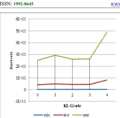
[image:6.612.321.535.111.311.2]Figure 6. Minimum, average, and maximum kurtosis values from KL-Grade 0 to KL-Grade 4
Figure 6 shows that the kurtosis values for each cluster ranged from 9.39×10⁶ to 2.51×10¹¹ (first cluster), -1.3×10⁷ to 2.93×10¹¹ (second cluster), -3.00×10⁷ to 2.59×10¹¹ (third cluster), -1.30×10⁷ to 2.62×10¹¹ (fourth cluster), and -2.9×10⁷ to 4.9×10¹¹ (fifth cluster).
Figure 7. Minimum, average, and maximum mean values from KL-Grade 0 to KL-Grade 4
Figure 7 portrays that the average mean values were directly proportional to the grade values. The average mean values for each cluster were 1.64×10⁹, 1.88×10⁹, 1.92×10⁹, 1.82×10⁹, and 2.13×10⁹ respectively. The range of the mean values for each cluster were 1.43×10⁹ to 1.82×10⁹ (first cluster), 1.66×10⁹ to 1.95×10⁹ (second cluster), 1.61×10⁹ to 2.33×10⁹ (third
cluster), 1.58×10⁹ to 1.99×10⁹ (fourth cluster), and 1.74×10⁹ to 2.32×10⁹ (last cluster).
Figure 8. Minimum, average, and maximum skewness values from KL-Grade 0 to KL-Grade
4
[image:6.612.90.300.392.583.2]Skewness values were different from the mean ones, of which these values tent to decrease along with the increase of KL-Grade values. In other words, skewness values were inversely proportional to the grade values. The skewness values for each cluster were 6.13×10⁹, 1.1×10⁷, 1.3×10⁷, 9.70×10⁷, and -2.00×10⁷ respectively. The range skewness values from the first to the last clusters were -9.40×10⁶ to -2.52×10⁶, -1.30×10⁶ to -6.27×10⁶, -3.0×10⁷ to -5.45×10⁶, -1.30×10⁷ to -4.97×10⁶, and -2.90×10⁷ to -7.93×10⁶ respectively.
[image:6.612.322.533.514.691.2]1965 Figure 9 exhibits that the ranges of variance values for each KL-Grade were 1.33×10¹¹ to 1.60×10¹¹, 1.17×10¹¹ to 1.48×10¹¹, 5.11×10¹⁰ to 1.51×10¹¹, 1.12×10¹¹ to 1.53×10¹¹, and 5.33×10¹⁰ to 1.40×10¹¹ respectively. The average variance values were 1.47×10¹¹, 1.25×10¹¹, 1.16×10¹¹, 1.31×10¹¹, and 8.49×10¹⁰.
The results of GLCM features from the extraction process were revealed in Figure 10 to 15. The range of energy values for each cluster were 6.26×10⁵ to 1.83×10⁶, 6.26×10⁵ to 1.83×10⁶, 6.26×10⁵ to 1.83×10⁶, 6.26×10⁵ to 1.83×10⁶, and 6.39×10⁵ to 1.75×10⁶. The average energy values from the first to the last cluster were 1.06×10⁶, 1.17×10⁶, 1.21×10⁶, 1.22×10⁶, and 1.48×10⁶ respectively.
[image:7.612.322.529.174.354.2]Figure 10. Minimum, average, and maximum energy values from KL-Grade 0 to KL-Grade 4
Figure 11. Minimum, average, maximum homogeneity values from Grade 0 to
KL-Grade 4
Figure 11 shows the homogeneity values for each cluster, which ranged from 6.80×10⁶ to 8.23×10⁶ (first cluster), 6.80×10⁶ to 8.23×10⁶ (second cluster), 6.80×10⁶ to 8.23×10⁶ (third cluster), 6.80×10⁶ to 8.23×10⁶ (fourth cluster), and 6.81×10⁶ to 8.88×10⁶ (last cluster).
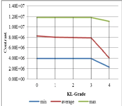
Figure 12. Minimum, average, and maximum contrast values from KL-Grade 0 to KL-Grade 4
Figure 12 conveys that the average contrast values for each cluster were 8.31×10⁶, 8.04×10⁶, 7.95×10⁶, 7.91×10⁶, and 4.05×10⁶ respectively. The range values from the first to the last cluster were 3.95×10⁶ to 1.18×10⁷, 3.95×10⁶ to 1.18×10⁷, 3.95×10⁶ to 1.18×10⁷, 3.95×10⁶ to 1.18×10⁷, and 2.26×10⁶ to 1.11×10⁷ respectively. The contrast values were inversely proportional to the KL-Grade values.
[image:7.612.90.299.300.472.2] [image:7.612.323.532.506.694.2]1966 Figure 13 portrays that the average mean i values for each cluster were 4.84×10⁷, 4.89×10⁷, 4.90×10⁷, 4.91×10⁷, and 5.87×10⁷ respectively. The minimum values for each cluster were 4.58×10⁷, 4.58×10⁷, 4.58×10⁷, 4.58×10⁷, and 4.97×10⁷ respectively, whereas, the maximum values were 5.24×10⁷, 5.24×10⁷, 5.24×10⁷, 5.24×10⁷, and 6.64×10⁷ respectively.
Figure 14. Minimum, average, and maximum mean j from KL-Grade 0 to KL-Grade 4
[image:8.612.90.302.505.697.2]Figure 14 shows that the average mean j values for each grade were 4.84×10⁷, 4.89×10⁷, 4.90×10⁷, 4.91×10⁷, and 5.87×10⁷. The range values for each cluster were from 4.58×10⁷ to 5.24×10⁷ (first cluster), 4.58×10⁷ to 5.24×10⁷ (second cluster), 4.58×10⁷ to 5.24×10⁷ (third cluster), 4.58×10⁷ to 5.24×10⁷ (fourth cluster), and 4.97×10⁷ to 6.64×10⁷ (fifth cluster).
Figure 15. Minimum, average, and maximum values of standard deviation from KL-Grade 0 to
KL-Grade 4
The average standard deviation values for each grade were 1.00×10⁹, 9.89×10⁸, 9.86×10⁸, 9.86×10⁸, and 9.78×10⁸ (see Figure 15). The minimum and maximum standard deviation values were respectively 8.54×10⁸ and 1.11×10⁹ (first cluster), 8.54×10⁸ and 1.11×10⁹, 8.54×10⁸ and 1.11×10⁹ (third cluster), 8.54×10⁸ and 1.11×10⁹ (fourth cluster), and 9.11×10⁸ and 1.14×10⁹ (last cluster).
Figure 16. Minimum, average, and maximum variance values from KL-Grade 0 to KL-Grade 4
Figure 16 shows that the average variance values from KL-Grade 0 to 4 were 6.48×10⁷, 6.62×10⁷, 6.66×10⁷, 6.68×10⁸, and 8.87×10⁹ respectively. The minimum and maximum variance values for each cluster were 4.94×10⁷ and 8.43×10⁷ (first cluster), 4.94×10⁷ and 8.43×10⁷ (second cluster), 4.94×10⁷ and 8.43×10⁷ (third cluster), 4.94×10⁷ and 8.43×10⁷ (fourth cluster), and 6.49×10⁷ and 1.07×10⁸.
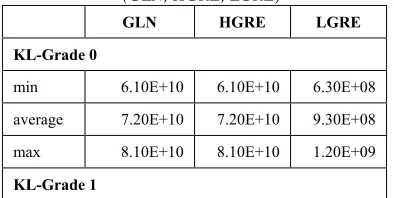
[image:8.612.322.519.628.727.2]The extraction results of GLRLM features from the first to the last cluster were revealed in Table 4. The features were then processed in learning process using LVQ.
Table 4. The Extraction Results Of GLRLM Features (GLN, HGRE, LGRE)
GLN HGRE LGRE KL-Grade 0
min 6.10E+10 6.10E+10 6.30E+08 average 7.20E+10 7.20E+10 9.30E+08 max 8.10E+10 8.10E+10 1.20E+09
1967
GLN HGRE LGRE
min 6.10E+10 6.10E+10 6.27E+08 average 7.12E+10 7.12E+10 9.22E+08 max 8.08E+10 8.08E+10 1.21E+09
KL-Grade 2
min 2.60E+10 2.60E+10 9.60E+08 average 5.10E+10 5.10E+10 1.20E+09 max 8.30E+10 8.30E+10 1.50E+09
KL-Grade 3
min 3.70E+10 3.70E+10 6.70E+08 average 5.70E+10 5.70E+10 1.10E+09 max 7.90E+10 7.90E+10 1.30E+09
KL-Grade 4
[image:9.612.82.536.41.739.2]min 2.56E+10 2.56E+10 1.01E+09 average 3.94E+10 3.94E+10 1.45E+09 max 8.26E+10 8.26E+10 1.69E+09
Table 5. The Extraction Results Of GLRLM Features (LRE, RLN, RP, SRE)
LRE RLN RP SRE KL-Grade 0
min 4.20E+07 1.70E+11 1.70E+07 5700814 average 7.20E+07 2.40E+11 2.00E+07 6238417 max 9.90E+07 3.40E+11 2.40E+07 6902381
KL-Grade 1
min 4.24E+07 1.73E+11 1.73E+07 5.70E+06 average 7.12E+07 2.51E+11 2.04E+07 6.28E+06 max 9.95E+07 3.39E+11 2.38E+07 6.90E+06
KL-Grade 2
min 4.30E+07 3.70E+10 7581563 3805069 average 3.20E+08 1.40E+11 1.40E+07 5074408 max 7.30E+08 3.50E+11 2.40E+07 7036315
KL-Grade 3
min 4.70E+07 6.10E+10 1.00E+07 4229569 average 1.80E+08 1.70E+11 1.60E+07 5423660 max 3.30E+08 3.10E+11 2.30E+07 6779000
KL-Grade 4
min 4.94E+07 3.17E+10 6.98E+06 3.56E+06 average 6.22E+08 8.45E+10 1.05E+07 4.39E+06
LRE RLN RP SRE
max 9.62E+08 2.89E+11 2.23E+07 6.56E+06
4. DISCUSSION
The learning process using LVQ was conducted through seven steps of experiment covering:
- Learning features of FO - Learning features of GLCM - Learning features of GLRLM
- Combined learning features of FO and GLCM
- Combined learning features of FO and GLRLM
- Combined learning features of GLCM and GLRLM
- Combined learning features of FO, GLCM, and GLRLM
The whole learning process used learning rate value of 0.5 and epoch values of 1000, 5000, 10000, and 15000. Table 6 shows the results of times required in the learning process. Results implied that the more times required in the process, the more increase the epoch values.
Table 6. Times Required In Learning Process Using LVQ
Epoch Time (second) Learning of FO features
1000 0.9204 5000 2.9796 10000 8.6581 15000 12.2929
Learning of GLCM features
1000 1.0920 5000 4.7424 10000 7.5348 15000 13.3069
Learning of GLRLM features
1000 1.0452 5000 4.5396 10000 4.9140 15000 6.1620
Learning of combined features between FO and GLCM
1000 0.9828 5000 4.5396 10000 7.9873 15000 12.9793
Learning of combined features between FO and GLRLM
1000 1.0296 5000 4.3836 10000 8.5177 15000 6.1932
Learning of combined features GLCM and GLRLM
[image:9.612.190.511.410.737.2]1968
Epoch Time (second)
5000 5.1636 10000 9.1105 15000 13.5565
Learning of combined features FO, GLCM and GLRLM
1000 0.9672 5000 5.1324 10000 8.2057 15000 8.4553
[image:10.612.89.297.248.469.2]After learning, we get the weight which is then used when testing. Accuracy obtained from the testing process as in Table 7.
Table 7. Accuration for each stage
Learning Stage Accuration (%)
Learning of FO features 24.012
Learning of GLCM
features 52.94
Learning of GLRLM
features 19.98
Learning of combined features between FO and
GLCM 18.862
Learning of combined features between FO and
GLRLM 51.28
Learning of combined features GLCM and
GLRLM 47.28
Learning of combined features FO, GLCM and
GLRLM 43.28
Globally, the best accuracy is determined by using GLCM. But in detail it is illustrated in Table 8.
Testing using FO ability to classify according to the cluster can best determine grade 2. Classification using the GLCM feature can best determine grade 4 which is 73% accuracy. y using RLM the ability to classify is lower by using the GLCM feature. RLM cannot classify grade 0 and grade 2. Applying a better result combination feature to recognize grade 4. All combination features produce 83.4% accuracy. But this combination feature has the disadvantage of being very difficult to classify in clusters 2 and 3.
Table 8. Accuration For Each Stage
Stage Accuration (%)
0 1 2 3 4
FO 34.65 23 50.98 9.43 2
Stage Accuration (%)
0 1 2 3 4
GLCM 33.3 83.4 50 25 73 RLM 0 16.6 0 33.3 50 FO+GLCM 33.66 0 50 8.69 1.96 FO+GLRLM 50 66 17 40 83.4 GLCM+RLM 50 66 20 17 83.4 FO+GLCM+RLM 50 66 0 17 83.4
5. CONCLUSION
The process of image processing, feature extraction, learning, and testing has been implemented. The best results obtained when using a system using LVQ based on GLCM features. But the disadvantage of this system is that it cannot recognize grade 2 well where recognizing grade 2 only results in an accuracy of only 50%. Based on this research, it is needed further research in order to obtain better accuracy.
ACKNOWLEDGEMENT
We would also like to show our gratitude to Ristek DIKTI Indonesia, Universitas Negeri Surabaya, and Osteoarhtritis Initiative (OAI) for supporting data.
REFERENCES:
[1] Mahajan, S Verma, V Tandon, Osteoarthritis, Journal of The Association of Physicians of India, Vol. 53 July 2005 pp. 634-641. [2]
https://radiopaedia.org/articles/kellgren-and- lawrence-system-for-classification-of-osteoarthritis-of-knee
[3] Mark D. Kohn, Adam A. Sassoon, Navin D. Fernando, Classifications in Brief: Kellgren-Lawrence Classification of Osteoarthritis, Clinical Orthopaedics and Related Research, Vol. 474(8) , 2016.
[4] Buckland-Wright, Current status of imaging procedures in the diagnosis, prognosis and monitoring of osteoarthritis, Bailliere's Clinical Rheumatology-- Vol. 11, No. 4, November 1997.
1969 [6] Tanna, Priority Medicines for Europe and
the World "A Public Health Approach to Innovation", Background Paper 6.12 Osteoarthritis,
https://www.who.int/medicines/areas/priorit y_medicines/BP6_12Osteo.pdf.
[7] Elders MJ. The increasing impact of arthritis on public health. J Rheumatol 2000;60(Suppl):6-8.
[8] Anifah, Purnomo, Hariadi, Purnama, Automatic Segmentation of Impaired Joint Space Area for Osteoatritis Knee on X-ray Image using Gabor Filter Based Morphology Process, IPTEK, Vol.22 No.3 2011, 117-176.
[9] Lior Shamir, Shari M. Ling, William W. Scott, Angelo Bos, Nikita Orlov, “Knee X-ray image analysis method for automated detection of Osteoarthritis,” pp. 1–10, 2008. [10] Anifah, Purnomo, Hariadi, Purnama,
Osteoarthritis Classification Using Self Organizing Map Based on Gabor Kernel and Contrast-limited Adaptive Histogram Equalization, The Open Biomedical Engineering Journal, February, Vol.7 2013, 18-28.
[11] R.T. Wahyuningrum, Purnomo, L. Anifah, Purnama, A novel hybrid of S2DPCA and SVM for knee osteoarthritis classification, Computational Intelligence and Virtual Environments for Measurement Systems and Applications (CIVEMSA), 2016 IEEE International Conference on,
27-28 June 2016 Hungaria,
http://ieeexplore.ieee.org/document/7524317 /
[12] Anifah, M H Purnomo, T L R Mengko, I K E Purnama, 2018, Osteoarthritis Severity Determination using Self Organizing Map Based Gabor Kernel, ICIEVE 2017, IOP Conf. Series: Materials Science and Engineering 306 (2018) 012071, pp 1-6. [13] Stachowiak, Wolski, Detection and
prediction of osteoarthritis in knee and hand joints based on the X-ray image analysis, Biosurface and Biotribology Vol.2 (2016) pp.162–172.
[14] Ostearhtritis Initiative, “Osteoarthritis.” , www.OAI.com, 2009
[15] R.M.Haralick, K. Shanmugam, R.M.Haralick, K. Shanmugam,, “Textural features for image classification,” IEEE
Trans. System Man. Cybernetics, vol.