Yarn Strength Modelling Using Adaptive Neuro-Fuzzy
Inference System (ANFIS) and Gene Expression
Programming (GEP)
A.R. Fallahpour1, A.R. Moghassem, PhD2
1Dept. of Mechanical Engineering, Faculty of Engineering, University of Malaya, Kuala Lumpur, MALAYSIA
2Dept. of Textile Engineering, Qaemshahr Branch, Islamic Azad University, Qaemshahr, IRAN
Correspondence to
A.R. Moghassem email: [email protected]
ABSTRACT
This study compares capabilities of two different modelling methodologies for predicting breaking strength of rotor spun yarns. Forty eight yarn samples were produced considering variations in three drawing frame parameters namely break draft, delivery speed, and distance between back and middle rolls. Several topologies with different architectures were trained to get the best adaptive neuro-fuzzy inference system (ANFIS) and gene expression programming (GEP) models. Prediction performance of the GEP model was compared with that of ANFIS using root mean square error (RMSE) and correlation coefficient (R2-Value) parameters on
the test data. Results show that, the GEP model has a significant priority over the ANFIS model in term of prediction accuracy. The correlation coefficient (R2
-value) and root mean square error for the GEP model were 0.87 and 0.35 respectively, while these parameters were 0.48 and 0.53 for the ANFIS model. Also, a mathematical formula was developed with high degree of accuracy using GEP algorithm to predict the breaking strength of the yarns. This advantage is not accessible in the ANFIS model.
Keywords: Breaking strength of rotor spun yarns –
Drawing frame – Adaptive neuro-fuzzy inference system - Gene expression programming – Mathematical formula
INTRODUCTION
Breaking strength of a yarn is an important quality parameter that affects determination of its applicable possibilities [1]. Raw material factors, process variables, machine parameters, and machine parts selection are four important groups of variables that affect yarn strength [2].
A survey of the literature revealed that, there has been a great deal of research done on roller drafting of staple fiber assemblies as an influencing factor on spun yarn properties [2]. The draw frame attenuates
sliver to the desired linear density and reduces irregularity by the process of doubling [3]. Drafting quality, governed by the process variables such as break draft, roller setting, delivery speed, and top arm pressure, affects fiber arrangement in a sliver, and its effect may be conveyed toward the fibrous assembly in spun yarn, influencing its structure and properties [2, 4]. However, there is a high degree of interaction between these variables and the quality of the product. For this complex process, a model that considers all the variables is not available [5].
Modelling of yarn properties is one of the most fascinating topics in textile research. A large number of prediction models have been exercised to prognosticate yarn properties such as strength [6]. Mathematical and statistical models are the first that are used in textile disciplines to explore relationships among variables and characteristics of the product [7]. Prediction performance of the mathematical models is limited for non-linear problems, due to the introduction certain simplifying assumptions. Also, statistical models do not provide as deep an understanding of the relationship between inputs and outputs [8, 9].
As a non-linear problem, prediction of the breaking strength of a yarn can be realized by an alternative modelling method such as the artificial neural network (ANN) [10, 11]. The widespread use of ANN has created a revolution in the domain of prediction modelling[9]. In recent years this method has been used extensively to model various properties of yarn and fabric. However, ANN models are called "black box," as they simply connect the inputs and outputs without giving a clear insight about the process [10, 11].
decision making. This kind of system could map the relationship between input and output parameters and generates some linguistic physical information about the process [9]. An adaptive neuro-fuzzy inference system (ANFIS) formed by amalgamating the fuzzy logic systems with the learning capabilities of ANN can enhance the accuracy and insight given by the prediction model [12]. Fuzzy logic based models can be developed by using the experience of the spinner only and they could provide good understanding about the roles played by various inputs on the outputs [6]. However, similar to ANN models, a neuro-fuzzy system is not able to exhibit quantitative relationship between variables. Therefore, it is desirable to develop a non-linear model with an explicit mathematical expression for accurate prediction of yarn strength.
Another soft computing approach from the family of evolutionary programming that is known as Gene Expression Programming (GEP) is also a promising candidate for complex prediction problems [13]. Studies show that, the performance of the GEP is much better than that of the statistical and ANN models [8, 14]. Also, GEP can provide prediction equations without requiring a cast equation as in the case of regression analysis [8, 13]. Given a set of linear and non-linear functions and a set of terminal variables, GEP can generate non-linear expressions with respect to the terminal variables. However, in the textile field, few applications of GEP have been reported [15].
In this study, GEP is employed to establish a mathematical formula for predicting the breaking strength of rotor-spun yarns based on three draw frame variables, namely, break draft, delivery speed, and distance between back and middle rolls. A neuro- fuzzy inference system (ANFIS) is also implemented for a comparison.
A BRIEF OVERVIEW OF GENETIC EXPRESSION PROGRAMMING (GEP)
Based on the evolutionary theory first introduced by Charles Darwin in 1859 [16], Holland discussed the original idea of using genetic algorithms in solving problems in 197517. This theory is based on the
survival of the fittest and is a starting point for evolutionary computation. With respect to the genetic algorithm, Koza in 1992 proposed genetic programming, which is in fact a subset of evolutionary computation [18].
GEP only needs the problem to be defined. Then the program searches for a solution in a problem-independent manner. The process begins with random generation of the chromosomes of each of the initial population. Then the chromosomes are expressed and the fitness of each individual is assessed. The individuals are then selected on the basis of fitness to reproduce with modification, leaving a progeny with a new train. The individuals of the new generation are subjected to the same developmental process until a solution has been found [13].
Genetic algorithm (GA) has different domains of applications in various engineering fields [19]. Nonetheless, offshoots of GA namely, gene expression programming, a natural development of genetic algorithm (GA) and genetic programming (GP) has not received attention by researchers.
Genetic expression programming (GEP) is an innovation in genetic programming. This method was introduced by Ferreira in 2001 [20]. GEP is a genetic algorithm because it uses populations of individuals, selects them according to fitness, and introduces genetic operation using one or more genetic operators. The fundamental difference between the three algorithms resides in the nature of the individuals: in GA the individuals are linear strings of fixed length (chromosomes); in GP the individuals are nonlinear entities of different sizes and shapes (parse trees); and in GEP the individuals are encoded as linear strings of fixed length (the genome or chromosomes) which are afterwards expressed as nonlinear entities of different sizes and shapes [20].
The advantages of GEP are: first, the chromosomes are simple entities: linear, compact, relatively small, and easy to be genetically manipulated (replicate, mutate, recombine, transpose) and second, the expression trees are exclusively the expression of the respective chromosomes.
FIGURE 1. A generic flowchart of the GEP algorithm.
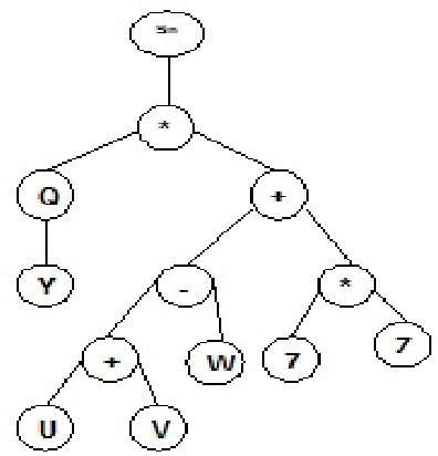
In GEP method, algebraic expression can be represented as an expression tree (ET). The ET representation is in fact the phenotype of GEP chromosomes (genotype). In algorithm GEP chromosomes decode into phenotype. Genotype and phenotype can be extracted from each other. Consider a typical GEP gene as follow:
V U Z W Y
Q. . .*. . .7. . . .
.
sin * (1)
WhereQrepresents square root function and "." separates element for easy reading.
sin,Q,*,,
and
Y,W,Z,U,V,7
are examples of function setFand terminal set T. ET of gene 1 has shown in
Figure 2.
Expression 1 is typically named as Karva notation or a K-expression [21]. To decode a gene into an expression tree (ET), the parity of each symbol is needed (variables and numerical constants are considered 0-parity) and associate each symbol with the parameters necessary for its evaluation [22].
FIGURE 2. Example of GEP expression tree (ET).
In the above example the first element requires one parameter (the second element, * that is written after sin ); the second element require two parameters (the third and the fourth element, Q,); the third element requires one parameter (the fifth element, Y); the fourth element requires two parameter (the sixth and the seventh element, , *); the fifth element requires no parameter, and so on. The mathematical form of the gene 1 is:
sin( Y* (((U V )W) (7 * ))) Z (2)
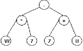
An ET can be translated into a K-expression by recording the nodes from left to right in each layer of ET, from root layer down to the deepest one to form the string. There are two parts: (1) redundant element and (2) ORF in each gene. Open reading frame (ORF) referred to useful part of the gene. Also useless part is called non-coding region [23]. Consider the follow gene:
.*. . .7. . . .sin.*. . . .W Z U V Q Y
(3)
The only difference between this gene and the previous gene is that the first 5 elements of gene 1 are rotated to the end of gene 3. In spite of the same length of 13, they have different valid K-expression length. The valid K-expression size of the gene 3 is 7. The mathematical form corresponding to gene 3 is:
( *7) (W Z U ) (4)
FIGURE 3. Example of GEP expression tree (ET).
Thus, in GEP, what varies is not the length of genes (which is constant) but the length of the ORF. To guarantee the validity of a randomly selected genome, GEP employs a head–tail method. Each GEP gene is composed of a head and a tail. The head may contain both function and terminal symbols, whereas the tail may contain only terminal symbols [20]. The size of the tail section is:
( 1) 1
t a h (5)
Where h is the size of the head section and
a
is
max arity f f( )| F . F T h, , and
n
(number of genes) are parameter of the GEP algorithm.In GEP, a new generation is created by operators. A chromosome might be modified by one or several operators at a time or not be modified at all.
There are several operators in GEP; selection, mutation, transposition, crossover (recombination), insertion sequence (IS) transposition, root IS transposition (RIS), and gene transposition. Mutation can happen anywhere in the chromosome. In the heads any element can change into another; in the tails terminals can only change into terminals. In crossover, two parent genomes are randomly chosen and paired to exchange some elements between them. There are three kinds of crossovers; one-point recombination, two-point recombination, and gene recombination [24]. Sequences of symbols that are called transposition are copied and inserted into some location by IS, RIS and gene transposition operators. The insertion point and the insertion sequence which they select are different.
A BRIEF OVERVIEW OF NEURO-FUZZY SYSTEM AND ANFIS
Some lacunas of the ANN modelling could be overcome by using fuzzy logic [6]. The foundation of fuzzy logic, which is an extension of crisp logic, was laid by Lotfi A. Zadeh at the University of California at Berkeley, USA. Unlike ANN models, fuzzy logic does not require an enormous amount of input-output
data [6]. In crisp logic, variables are true or false. A fuzzy set contains elements with only partial membership ranging from 0 to 1 to define uncertainty for classes that do not have clearly defined boundaries. For input and output variables of a fuzzy inference system (FIS), the fuzzy sets are generated by dividing the universe of discourse into a number of sub-regions. A classical set may be expressed as follows:
xx6
A (1) (6)
If Xis the universe of discourse and its elements are denoted byx, then a fuzzy setAinXis defined as a set of ordered pairs as:
x x x X
A ,A( ) (7)
WhereA(x)is the membership function ofxinA[12].
Once the fuzzy sets are chosen, a membership function for each set should be created. A membership function is a typical curve that converts the numerical value of input within a range from 0 to 1, indicating the belongingness of the input to a fuzzy set. This step is known as ‘fuzzification’. Membership function can have various forms, such as triangle, trapezoid and Gaussian. Triangular membership function is the simplest one and it is a collection of three points forming a triangle. Definition of triangular membership function is as follow [6].
m x L for L m
L x
otherwise R x m for m R
x R x A
0 ) (
(8)
Where m is the most promising value, L and R are the left and right spread (the smallest and largest value that x can take).
b x a a b a x d x a x for d x c c d x d c x b for x A , 0 1 ) ( (9)
The Gaussian membership function depends on two parameters namely standard deviation (σ) and mean (μ) and is represented as shown below [6].
2 2 2 ) ( ) ( x e x A (10)
Fuzzy linguistic rules provide quantitative reasoning that relates input fuzzy sets with output fuzzy sets. A fuzzy rule base consists of a number of fuzzy if-then rules. For example, in the case of two-input and single-output fuzzy system, it can be expressed as shown below [6].
If x is high and y is medium then z is low, where x, y
and z are variables representing two inputs and one output; high, medium and low are the fuzzy sets of x,
y and z, respectively.
The output of each rule is also a fuzzy set. Output fuzzy sets are then aggregated into a single fuzzy set. This step is known as ‘aggregation’. Finally, the resulting set is resolved to a single crisp number by ‘defuzzification’. There are several methods of defuzzification like centroid, centre of sums, mean of maxima and left-right maxima. However, centroid method of defuzzification is generally used in most of the cases and it is done as shown below [6].
dx x xdx x x A A ) ( ) ( *
(11)Where x* is the defuzzified output and μA(x) is the output fuzzy set after aggregation of individual implication results [6].
The ANFIS is the hybrid neuro-fuzzy system which was developed by Jang in 1993. ANFIS combines the fuzzification technique of fuzzy logic with the
learning capability of ANN to facilitate the hybrid learning procedure [25]. Fuzzification maps an input value to fuzzy sets in a certain universe of discourse. This can make the neuro-fuzzy model fit the training set of input-output data more accurately. Neural network technique aids the fuzzy modeling procedure to learn the information about the data set and computes the membership function parameters that best allow the associated FIS to track the given input-output data. ANFIS (adaptive neuro-fuzzy inference system) is a class of adaptive network that is functionally equivalent to FIS. Using a given input-output data set, ANFIS constructs a FIS whose membership function parameters are tuned (adjusted) using either a back-propagation algorithm or a hybrid learning algorithm (a combination of back-propagation and least squares method) [9, 12, 26].
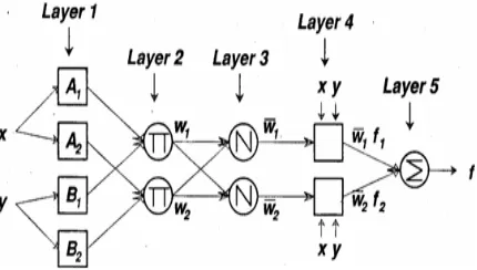
Supposed ANFIS with five layers has a Takagi-Sugeno,s type as shown in Figure 4.
FIGURE 4. ANFIS architecture.
Each layer consists of a number of nodes that perform different operations according to the internal node function. The nodes of the same layer have similar functions. Based on the above figure, it is
assumed that there are two inputsxand yand only one outputz. A common two fuzzy if–then rules in first-order Sugeno,s type are as below:
(12) 2 2 2 2 2
2 ( , )
:
1 ifx Aandy Bthen f x y p x q y r
Rule (13)
Layer 1: Every node i in this layer is a square node with a node function
) (
1 x
Oi Ai (14)
Where x is the input to node i and Ai is a linguistic layer associated with this node.
1 1 1 1
1
1 ( , )
:
1 ifx Aandy Bthen f x y px qy r
Layer 2: Each node in this layer is a fixed node labelled π, whose output is the product of all of the incoming signals.
2 , 1 , ) ( ) (
2 x y i
Oi Ai Bi (15)
Each node in this layer represents the firing strength of a rule.
Layer 3: Every node in this layer is a circle node labeled
N. The ith node calculates the ratio of the ithrule’s firing strength to the sum of all rules’ firing strengths:
2 , 1 ,
2 1
i
w w
wi
(16)
For convenience, outputs of this layer will be called called normalized firing strengths.
Layer 4: Every node i in this layer is a square node with a node function, as shown below:
) (
4
i i i i i i
i f px qy r
O (17)
Where i is the output of layer 3, and (pi,qi,,ri)is the parameter set. Parameters in this layer will be referred to as consequent parameters.
Layer 5: The single node in this layer is a fixed node labelled Σ that computes the overall output as the summation of all of the incoming signals [27]:
i i i
i i
i i
i
w f w f
output overall
O15
(18)
MATERIALS AND METHODS
Sample Yarn Production and Experiment
The data used in the GEP and ANFIS models were collected from 48 rotor spun yarn samples. Cotton fiber with 27 mm mean fiber length, 3.6 micronaire fineness, and fiber maturity index of 0.85 were furnished as a second drawing frame sliver with linear density of 5.2ktex. The 30Ne yarn was spun on a Rieter RU04 rotor spinning machine with 900tpm. The opening roller speed was 8200rpm. The 35 mm diameter rotor worked at a speed of 75000rpm.
Effect of three main variable parameters in the draw frame (passage No.1) namely, delivery speed, break draft, and distance between back and middle rolls on breaking strength of the yarns was studied. Delivery speed was changed in four levels: 550, 650, 700 and750 m/min. Distance between back and middle rolls was set in four values: 8, 10, 12 and 14 mm. Break draft was selected at 1.14, 1.41 and 1.70.
Forty eight different yarn samples were produced as shown in Table I. Tensile characteristics of the yarns were examined with Uster Tesorapid 3. A test specimen of 500 mm was elongated at an extension rate of 500 mm/min. The average values of the experiments are shown in Table I.
TABLE I. Specifications and quality parameters of the cotton rotor-spun-yarn samples.
Sample Variables B.S Sample Variables B.S Sample Variables B.S
D.B.B.M.R D.S B.D D.B.B.M.R D.S B.D D.B.B.M.R D.S B.D
A1 14 650 1.14 11.94 A17 12 750 1.41 13.73 A33 10 750 1.14 14.50 A2 8 650 1.14 12.30 A18 14 750 1.14 13.75 A34 14 750 1.41 14.50 A3 8 650 1.41 12.54 A19 12 650 1.41 13.80 A35 12 550 1.14 14.59 A4 14 650 1.41 12.69 A20 10 650 1.70 13.90 A36 8 750 1.41 14.60 A5 10 650 1.14 12.70 A21 8 550 1.70 13.95 A37 10 750 1.70 14.81 A6 8 700 1.14 12.83 A22 12 750 1.70 14.07 A38 14 550 1.70 14.81 A7 8 700 1.41 13.07 A23 12 550 1.41 14.10 A39 10 550 1.41 14.84 A8 8 650 1.70 13.12 A24 12 650 1.70 14.14 A40 14 700 1.70 14.91 A9 8 550 1.14 13.13 A25 12 750 1.14 14.22 A41 10 700 1.41 14.98 A10 14 650 1.70 13.23 A26 10 550 1.14 14.27 A42 10 750 1.41 15.00 A11 10 650 1.41 13.25 A27 14 550 1.41 14.27 A43 12 700 1.41 15.00 A12 8 550 1.41 13.37 A28 12 650 1.14 14.30 A44 10 550 1.70 15.02 A13 14 550 1.14 13.53 A29 8 750 1.14 14.36 A45 14 750 1.70 15.04 A14 8 750 1.70 13.56 A30 10 700 1.14 14.37 A46 12 700 1.70 15.34 A15 14 700 1.14 13.62 A31 14 700 1.41 14.37 A47 12 700 1.14 15.50 A16 8 700 1.70 13.65 A32 12 550 1.70 14.44 A48 10 700 1.70 15.55 D.B.B.M.R: distance between back and middle rolls (mm), D.S: delivery speed (m.min-1), B.D: break draft B.S: breaking strength (cN/tex)
Model Inputs and Outputs
The basic parameters of draw frame namely, delivery speed, break draft, and distance between back and middle rolls constitute the input parameters of the models. In the developed models X1 is break draft; X2 is
delivery speed and X3 is distance between back and
middle rolls. Yarn samples were tested for breaking strength using a Uster Tensorapid 3. This parameter constitutes the output parameter of the models (Y).
Modeling Methodologies
Optimization of ANFIS Parameters
For neuro-fuzzy modelling, neuro-solution software (version 5) was used. For the ANFIS model, various forms of membership functions were tried, and the Gaussian form was found to give the best prediction accuracy. While choosing the number of membership function, attention was made to keep the number of rules at such a level that they could be adequately trained using the available training data set, and it was ascertained that two membership functions would be used for each input variable. In the best ANFIS model, the number of membership function per input was 2. Also, fuzzy structure (fuzzy model), transfer function, epoch, learning rule, step size, and momentum were respectively 2, TSK, tan-h (x), 2000, momentum, 1 and 0.7.
In this study, an eight-fold cross-validation technique was applied to all the models. The training and testing were performed eight times. The data set of 48 samples was divided randomly into 8 subsets each containing of 6 samples. The subsets were combined together and eight sets of training and testing data were designed. Each time, seven subsets were used as the training set and one subset as testing set. Consequently, each designed network was trained and tested eight times. After training the model (the best structure) with different sets of data, the root mean square error of test and train data were measured by presenting them to the trained network. Then the average of root mean square errors of testing subsets was considered to achieve the model accuracy. Table II shows the structure of the best and some of the other ANFIS algorithms that were used for predicting breaking strength of the samples.
TABLE II. The parameters used in the ANFIS algorithm for different considered structures.
Parameters Models
1 2 3 4 5 6 7 8 9 10
Membership function G G B B G B B G G B
Membership function per
input 2 1 2 3 2 10 3 6 7 5
Fuzzy structure (fuzzy model) TSK TSK TSK TSU TSU TSK TSK TSK TSU TSU Transfer function T(x) T(x) S(x) L(x) LT(x) T(x) T(x) LS(x) SMA(x) L(x)
Epoch 2000 2000 2000 2000 2000 2000 2000 2000 2000 2000
Learning rule M M M S QP M M LBM DBD CG
Step size 1 1 1 ---- 1 1 1 ---- 1 ----
Momentum 0.7 0.7 0.7 ---- 0.5 0.7 0.7 ---- 0.1 ----
Additive ---- ---- ---- ---- ---- ---- ---- ---- 0.1 ----
Multiplicative ---- ---- ---- ---- ---- ---- ---- ---- 0.5 ----
Smoothing ---- ---- ---- ---- ---- ---- ---- ---- Gaussian ----
G: Gaussian B: Bell TSU: Takagi-Sugeno TSU: Takagi-Sukamoto T(x): Tangent-hyperbolic(x) S(x): Sigmoid(x) L(x): Linear(x) LT(x): Linear tangent-hyperbolic(x) LS(x): Linear-sigmoid(x) SMA (x): Soft Max Axon(x)
M: Momentum S: Step QP: Quick propagation LBM: Level berg marqua DBD: Delta bar delt CG: Conjugrate gradient
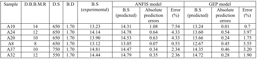
TABLE III. The experimental and predicted value of breaking strength of testing samples in third class of training using the best ANFIS and GEP structure.
Sample D.B.B.M.R D.S B.D B.S
(experimental) B.S ANFIS model GEP model (predicted)
Absolute prediction
errors
Error (%)
B.S (predicted)
Absolute prediction
errors
Error (%)
A10 14 650 1.70 13.23 14.31 1.08 7.54 13.24 0.01 0.7
A24 12 650 1.70 14.14 14.78 0.64 4.33 13.60 0.54 3.97
A20 10 650 1.70 13.90 14.53 0.63 4.33 13.66 0.24 1.75
A8 8 650 1.70 13.12 13.05 0.07 0.53 12.67 0.45 3.55
A37 10 750 1.70 14.81 14.47 0.34 2.34 14.35 0.46 3.20
A32 12 550 1.70 14.44 14.79 0.35 2.36 14.72 0.28 1.90
Model Construction and Analysis Using GEP Algorithm
GEP offers new possibilities to solve more complex technological and scientific problems. GEP algorithms represent nature more faithfully and therefore can be used as computer models of natural evolutionary processes. In this concern, the experimental data shown in Table I and the mentioned variables were employed to model breaking strength of the same yarn samples. The same eight sets used for evaluating ANFIS model were used in a GEP algorithm. Then, the resulting eight models were applied to the testing data sets.
The major task is to define the hidden function connecting the input variables (X1, X2, X3) and output
variable (Y). This can be written in the form of Y = f (X1, X2, X3). The function developed by GEP can be used to predict yarn strength. There were many
different combinations of parameters which mean many GEP models. Since, running the GEP for all of them requires a long computational time, a subset of these combinations was selected to investigate the performance of the GEP in predicting breaking strength of the yarns.
TABLE IV. The parameters used in the GEP algorithm for different considered structures.
Parameters Models
1 2 3 4 5 6 7 8 9 10
number of generation 3000 to 5000
population size 30 30 30 30 30 30 30 30 30 30
number of gene 3 5 7 6 8 9 10 9 8 7
head size 6 3 4 5 6 4 2 2 4 6
linking function + + - * + + + - / /
mutation rate 0.44 0.44 0.44 0.44 0.44 0.44 0.44 0.44 0.44 0.44
on-point recombination 0.3 0.3 0.3 0.3 0.3 0.3 0.3 0.3 0.3 0.3
two-point recombination 0.3 0.3 0.3 0.3 0.3 0.3 0.3 0.3 0.3 0.3
gene recombination rate 0.1 0.1 0.1 0.1 0.1 0.1 0.1 0.1 0.1 0.1
gene transportation rate 0.1 0.1 0.1 0.1 0.1 0.1 0.1 0.1 0.1 0.1
R-square on test data 0.98 0.57 0.82 0.27 0.23 0.61 0.10 0.22 0.64 0.64
MSE on test data 0.13 0.26 0.30 0.45 0.50 0.20 0.70 0.42 0.14 0.58
R-square on train data 0.69 0.65 0.64 0.30 0.72 0.82 0.35 0.47 0.65 0.63
MSE on train 0.24 0.27 0.30 0.55 0.21 0.13 0.50 0.47 0.30 0.29
Bold entries represent optimal setting
RESULTS AND DISCUSION
Correlation coefficient (R2-value) and root mean
square error (RMSE) were used for evaluating and comparing the prediction performance of ANFIS and GEP models. The results of two algorithms for predicting training and testing data sets are shown in
Table VI.
21 1
i n
i
p
i o
o n
RMSE (19)
Where, nis the number of pairs, oiand opare ith
desired output and calculated output, respectively.
The obtained results of average MSE and R2-value of
eight subsets of testing data indicated that the performance of GEP model was better than that of ANFIS model.
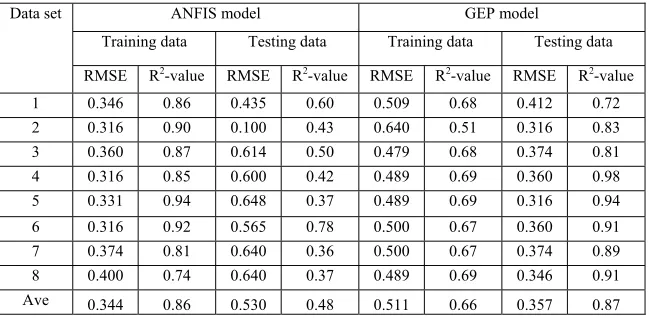
TABLE V. Performance of ANFIS architecture and GEP model with the best architecture on training and testing data sets.
Data set ANFIS model GEP model
Training data Testing data Training data Testing data
RMSE R2-value RMSE R2-value RMSE R2-value RMSE R2-value
1 0.346 0.86 0.435 0.60 0.509 0.68 0.412 0.72 2 0.316 0.90 0.100 0.43 0.640 0.51 0.316 0.83 3 0.360 0.87 0.614 0.50 0.479 0.68 0.374 0.81 4 0.316 0.85 0.600 0.42 0.489 0.69 0.360 0.98 5 0.331 0.94 0.648 0.37 0.489 0.69 0.316 0.94 6 0.316 0.92 0.565 0.78 0.500 0.67 0.360 0.91 7 0.374 0.81 0.640 0.36 0.500 0.67 0.374 0.89 8 0.400 0.74 0.640 0.37 0.489 0.69 0.346 0.91
Ave 0.344 0.86 0.530 0.48 0.511 0.66 0.357 0.87
The difference between the RMSE values of two models for predicting breaking strength of testing data was 0.173 (32.64%). Also, difference between the R2-values of two models on testing data was 0.39
(81.25%). In relation to breaking strength, the maximum and minimum RMSE in the ANFIS model for predicting testing data belonged to the fifth and
TABLE VI. Comparison of MSE and R2-value between ANFIS and GEP models.
Data RMSE R2-value
ANFIS GEP Difference (%) ANFIS GEP Difference (%) For training data 0.344 0.511 0.167(48.54) 0.86 0.66 0.20(23.25)
For testing data 0.530 0.357 0.173(32.64) 0.48 0.87 0.39(81.25)
Prediction Performance of Models
Since the testing is done using one of the data sets used to train and test the models during development, these models need to be tested using an independent data set outside of those used during development. To validate the models we used data that had not been used in model development (testing or training). This will provide a good understanding of how the model works outside the zone of development. The
prediction performance of the models was assessed using an independent test set similar to other published paper [28]. A set of six number of randomly selected yarn samples constituted the test set. From the prediction results, statistical performance indicators (RMSE and R2-value) were
calculated. The results are shown in Table VII, for both training and testing data sets.
TABLE VII. Comparison between the prediction power of two models on independent testing data.
Models Training data Testing data
RMSE R2-value RMSE R2-value Prediction error
Min (%) Max (%)
ANFIS 0.316 0.90 0.648 0.37 0.04(0.27) 1.41(9.41)
GEP 0.489 0.69 0.316 0.93 0.04(0.28) 0.53(4.00)
Difference 0.173(54.74) 0.21(23.33) 0.332(51.23) 0.56(151.35) --- ---
Table VII shows that, the difference between the RMSE values for predicting breaking strength of testing data was 0.332 that is 51.23%. Also, the difference between the R2-values for predicting breaking strength of testing data was 0.56 that is 151.35%. Details of testing data have been presented
in Table VIII. The ability of the best ANFIS model to predict the testing data is shown in Figure 5
schematically. Results reveal that, minimum and maximum prediction errors in the best ANFIS model are respectively 0.27% and 9.41%.
TABLE VIII. Prediction performance of independent test set carpets.
Sample D.B.B.M.R D.S B.D B.S (experimental)
ANFIS model GEP model
B.S (predicted)
Absolute prediction
errors
Error (%)
B.S (predicted)
Absolute prediction
errors
Error (%)
A39 10 550 1.41 14.84 14.61 0.23 1.57 14.50 0.34 2.34
A33 10 750 1.14 14.50 14.20 0.3 2.11 14.38 0.12 0.83
A30 10 700 1.14 14.37 14.68 0.31 2.11 14.43 0.06 0.41
A27 14 550 1.41 14.27 14.31 0.04 0.27 14.23 0.04 0.28
A14 8 750 1.70 13.56 14.97 1.41 9.41 14.03 0.47 3.34
11.5 12 12.5 13 13.5 14 14.5 15 15.5
1 2 3 4 5 6
Test data
B
reak
ing s
tr
engt
h (c
N
/t
e
x
)
Breaking strength (experimental) Breaking strength (predicted)
FIGURE 5. Evaluation of the ANFIS model to predict the breaking strength of the yarn samples.
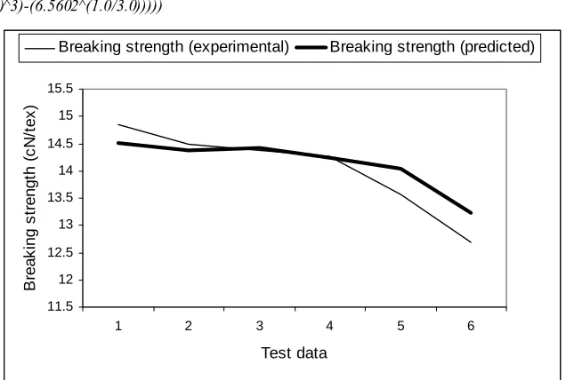
The performance of the best gene expression programming architecture on the same testing data is shown in Figure 6. The equation 20 represents the mathematical function generated by the best structure of GEP approach.
(20)
In this equation, d(1), d(2) and d(3) are equivalent to
X1, X2 and X3 that were inputs of the models. As it is
clear in Figure 6, there was a closer match between the actual and predicted breaking strength values than ANFIS model.
11.5 12 12.5 13 13.5 14 14.5 15 15.5
1 2 3 4 5 6
Test data
B
re
a
k
in
g
s
tr
e
n
g
th
(
c
N
/te
x
)
Breaking strength (experimental) Breaking strength (predicted)
FIGURE 6. Evaluation of the GEP model to predict the breaking strength of the yarn samples.
Based on the obtained results, minimum and maximum prediction errors in the best GEP model were 0.28% and 4.00%, respectively. Therefore, the GEP function was able to closely follow the trend of the actual data. All the data in Table VII and Figure 5
and Figure 6 confirmed the excellent capability of GEP model in predicting breaking strength of the yarn samples, compared with ANFIS model. The better performance of GEP algorithm could be
))))) 2^(1.0/3.0 ^3)-(6.560
sin(((X(3) (X(1)
2.6977) X(2))^2))
7324) -2.6977-3. (atan((((
)) sin(X(2))) 23*7.3695)
sin(((9.64 (7.3695
Y
explained based on the method of optimization of its parameters which was based on genetic algorithm.
Finally, presenting a specific mathematical equation describing the relation between dependent and independent parameters was a time consuming process, especially when there was not any clear relationship between input and output parameters. But, this case is easily obtainable by GEP algorithm. The GEP algorithm results in an equation that can be easily programmed even into a pocket calculator to use in future predictions. All of the obtained results accompanied with this benefit, demonstrate the advantages of GEP model when compared with ANFIS model.
CONCLUSION
In this study, gene expression programming (GEP) algorithm, as an intelligent methodology, was applied to obtain a prediction model for breaking strength of rotor spun yarns based on the three drawing frame parameters. Adaptive neuro-fuzzy inference system (ANFIS) model was also developed as a criterion to evaluate the prediction power of GEP algorithm. The obtained results from extensive computational tests indicate better prediction performance of the GEP model compared to the ANFIS model. The difference between the RMSE and R2-value of two proposed
models in predicting testing data was 0.173(32.64%) and 0.39(81.25%). GEP was found as a powerful programming algorithm in predicting breaking strength of rotor spun yarns. Also, another advantage of GEP is its ability to explore mathematical equations that can be used during the yarn producing process.
REFERENCES
[1] Sette, S.; Boullart, L.; Langenhove, A. V.; Kiekens, P.; Optimizing the Fibre-to-Yarn Production Process with a Combined Neural Network/Genetic Algorithm Approach;
Textile Research Journal 1997, 67, 84-92. [2] Plonsker, H. R.; Backer. S.; The Dynamics of
Roller Drafting, Part I: Drafting Force Measurement; Textile Research Journal
1967, 37, 673-687.
[3] Das, A.; Ishtiaque, S. M.; Niyogi, R.; Optimization of Fibre Friction, Top Arm Pressure and Roller Setting at Various Drafting Stages; Textile Research Journal
2006, 76, 913-921.
[4] Balasubramanian, N.; The Effect of Roller Weighting, Apron Spacing and Top-Roller Setting Upon Yarn Quality; Textile Research Journal 1975, 45, 322-325.
[5] Silva, E. A.; Paiva, A. P.; Balestrassi, P. P.; Silva, C. E. S.; New Modelling and Process Optimisation Approach for the False-Twist Texturing of Polyester; Fibres and Textiles in Eastern Europe 2009, 17, 57-62.
[6] Majumdar, A.; Ghosh. A.; Yarn Strength Modelling Using Fuzzy Expert System;
Journal of Engineered Fibres and Fabrics
2008, 3, 61-68.
[7] Erol, R.; Sagbas, A.; Multiple Response Optimisation of the Staple-Yarn Production Process for Hairiness, Strength and Cost;
Fibres and Textiles in Eastern Europe 2009, 17, 40-42.
[8] Baykasoglu, A.; Oztas, A.; Ozbay, E.; Prediction and Multi-Objective Optimization of High-Strength Concrete Parameters via Soft Computing Approaches; Expert Systems with Applications 2009, 36, 6145-6155.
[9] Majumdar, A.; Majumdar, P. K.; Sarkar, B.; Application of Linear Regression, Artificial Neural Network and Neuro-Fuzzy Algorithms to Predict the Breaking Elongation of Rotor-Spun Yarns; Indian Journal of Fibers & Textile Research 2005, 30, 19-25.
[10] Chen, T.; Zhang, C.; Chen, X.; Li, L.; A Soft Computing Model for Predicting Yarn Breaking Strength; Research Journal of Textile and Apparel 2007, 11, 80-86.
[11] Rajamanickam, R.; Hansen, S.; Jayaraman, S.; Analysis of the Modelling Methodologies for Predicting the Strength of Air-jet Spun Yarns; Textile Research Journal 1997, 67, 39-44.
[12] Majumdar, A.; Majumdar, P. K.; Sarkar, B.; Application of an Adaptive Neuro-fuzzy System for the Prediction of Cotton Yarn Strength from HVI Fiber Properties; Journal of the Textile Institute 2005, 96, 55-60. [13] Dayik, M.; Prediction of Yarn Properties
Using Evaluation Programming; Textile Research Journal 2009, 79, 963-972.
[14] Baykasoglu, A.; Dereli, T.; Tanis, S.; Prediction of Cement Strength Using Soft Computing Techniques; Cement and Concrete Research 2004, 34, 2038-2090. [15] Chen, Z. H.; Xu, B. G.; Chi, Z. R.; Feng, D.
G.; Mathematical Formulation of Knitted Fabric Spirality Using Genetic Programming;
Textile Research Journal 2012, 82, 667-676. [16] Darwin, C.; On the Origin of Species by
[17] Holland, J. H.; Adaptation in Natural and Artificial Systems, University of Michigan Press, 1975.
[18] Koza, J. R.; Genetic Programming: on the Programming of Computers by Means of Natural Selection, Cambridge (MA), MIT Press, 1992.
[19] Majumdar, A.; Mitra, A.; Banerjee, D.; Majumdar, P. K.; Soft Computing Applications in Fabrics and Clothing; A Comprehensive Review; Research Journal of Textile and Apparel 2010, 14, 1-17.
[20] Ferreira, C.; Gene Expression Programming; A New Adaptive Algorithm for Solving Problems; Complex Systems 2001, 13, 87-129.
[21] Ferreira, C.; Gene Expression Programming: Mathematical Modeling by an Artificial Intelligence. 2nd ed, Germany, Springer, 2006.
[22] Cranganu, C.; Bautu, E.; Using Gene Expression Programming to Estimate Sonic Log Distributions Based on the Natural Gamma Ray and Deep Resistivity Logs: A Case Study From the Anadarko Basin, Oklahoma. Journal of Petroleum Science and Engineering 2010, 70, 243–255.
[23] Tang, C. J.; Duan, L.; Peng, J.; The Strategies to Improve Performance of Function Mini-genetic Modifying, Overlapped Gene, Back-tracking and Adaptive Mutation. DEWJ06 (DBSJ Annual Conference), Invited talk and paper, Okinawa, Japan, 2006.
[24] Kauko, T.; On Current Neural Network Applications Involving Spatial Modeling of Property Prices, Journal of Housing and the Built Environment 2003, 18, 159–181.
[25] Eogratias Nurwaha, D.; Wang, X. H.; Prediction of Rotor Spun Yarn Strength from Cotton Fiber Properties Using Adaptive Neuro-Fuzzy Inference System Method, Fibers and Polymers 2010, 11, 97-100.
[26] Ghosh, A.; Forecasting of Cotton Yarn Properties Using Intelligent Machines;
Research Journal of Textile and Apparel
2010, 14, 55-61.
[27] Jang, J. S. R.; ANFIS: Adaptive-Network-Based Fuzzy Inference System, IEEE Transactions on Systems, Man, and Cybernetics 1993, 23, 665-683.
[28] Behera, B. K.; Guruprasad, R.; Predicting Bending Rigidity of Woven Fabrics Using Artificial Neural Networks, Fibers and Polymers 2010, 11, 1187-1192.
AUTHORS’ ADDRESSES Alireza Fallahpour
Department of Mechanical Engineering Faculty of Engineering
University of Malaya Kuala Lumpur 50603 MALAYSIA
Abdolrasool Moghassem, PhD
Department of Textile Engineering Qaemshahr Branch
Islamic Azad University Qaemshahr