Forestry & Natural-Resource Sciences Last Correction: Mar. 31, 2017
THE DEVELOPMENT OF A SPATIO-TEMPORAL MODEL FOR
WATER HYACINTH BIOLOGICAL CONTROL STRATEGIES
Hel´
ene Van Schalkwyk
1, Linke Potgieter
1, Cang Hui
2,3 1Department of Logistics, Stellenbosch University, South Africa 2
Department of Mathematical Sciences, Stellenbosch University, South Africa 3
African Institute for Mathematical Sciences, South Africa
Abstract.A reaction-diffusion model for a temporally variable and spatially heterogeneous environment
is developed to mathematically describe the spatial dynamics of water hyacinth and the interacting populations of the various life stages of theNeochetina eichhorniae weevil as a biological control agent on a bounded two-dimensional spatial domain. Difficulties encountered during the implementation of the model in Matlabare discussed, including the implementation of time delays and spatial averaging. Conceptual validation tests indicate that the model may succeed in describing the spatio-temporal dynamics of the water hyacinth and weevil interaction. A modelling framework is thereby provided to evaluate the effectiveness of different biological control release strategies, providing guidance towards the optimal magnitude, timing, frequency and distribution of agent releases. Numerical results confirm the hypothesis that the seasonal timing of releases have a significant influence on the success of the control achieved. However, in order to ascertain the degree to which the model output realistically represent the real life water hyacinth and weevil interaction, predictive validation tests are proposed for further research.
Keywords: Biological control, water hyacinth, reaction-diffusion model, optimal release strategy
1
Introduction
Water hyacinth, Eichhornia crassipes (Martius) Solms-Laubach (Pontederiaceae), has since the 1880s been distributed from its Amazonian origin to all parts of the world. Today it is regarded as one of the world’s, as well as South Africa’s, worst aquatic weeds. With its exponentially high growth rate, water hyacinth rules still or slow-moving water bodies by forming dense im-penetrable mats across the surfaces, having serious con-sequences for man and animal. Given enough space and favourable growing conditions (tropical weather, warm temperatures and water with high nutrient levels), the number of plants may double in a matter of a week, giving water hyacinth the ability to outgrow any native species occurring in the system. Seeds can remain vi-able after 15 – 20 years of remaining in water sediments [12, 15]. These characteristics make water hyacinth an extremely difficult weed to control.
Over the past century, mechanical, chemical and manual control methods proved to be both very expens-ive and ineffectexpens-ive, especially for large infested water bodies. These concerns motivated a more serious con-sideration of the use of biological control methods [13].
Biological control entails the sourcing of natural enemies from the weed’s native land and putting them through quarantine where their host specificity is assessed. If proven to be host specific, they are certified for release as biological control agents (BCAs) for the specific weed. Candidate species are then released in the new habitat where they feed on the weed, thereby contributing to the suppression of the alien plant population. After extens-ive research began in Argentina in 1961, the first water hyacinth host-specific natural enemies were released as BCAs in the USA in the early 1970s. Since then several BCAs have been released in 33 countries [13]. Biological control trumps other methods by offering a more sus-tainable, long-termed, environment-friendly and more affordable solution to the water hyacinth problem, even for large or inaccessible areas [10].
Apart from the classical biological control approach, where BCAs are released in the field directly out of quar-antine, the use of mass rearing technology in biological control has become more common. BCAs that have been cleared from quarantine are taken to a mass rear-ing facility where aquatic weed BCAs are reared in large numbers on their host plants in portable pools,
mak-Copyright c2017 Publisher of theMathematical and Computational Forestry & Natural-Resource Sciences
ing more frequent releases possible in order to speed up biological control [3]. Inadequate release methods may cause non-establishment of BCAs or unsuccessful con-trol [10]. Therefore, implementing the best timing, fre-quency, magnitude and distribution for releases are vital to a successful biological control programme.
The biological control of water hyacinth in South Africa currently relies on six agents of which the popular Neochetina eichhorniae Warner (Coleoptera: Curculionidae) weevil species is considered in this pa-per. The sound and effective management of the wa-ter hyacinth weed remains a challenge in South Africa [3]. A local mass rearing facility from the Cape Town Invasive Species Unit in Westlake commenced with weekly releases of BCAs at the nearby Kuils-river site in March 2015 [14]. After one and a half years of BCA releases, consisting of mostly Megamelus scutellaris Berg (Hemiptera: Delphacidae) (more than 380 000) and a few Neochetina bruchi Hustache (Cole-optera: Curculionidae) weevils (about 2 600), the site was still completely covered with water hyacinth, with little evidence of the impact of BCAs. Suggestions to-wards more effective release strategies for different tem-perature conditions may aid in improving the control of the weed. Byrne et al. [2] agrees that flawed or inap-propriate release procedures contribute to the variable success of biological control programmes for water hy-acinth. It is hypothesized that the timing of releases, both in terms of seasonality and frequency of releases, have a significant influence on the success of the control achieved.
In this paper, a mathematical model, describing the water hyacinth and N. eichhorniae weevil population growth, dispersal and interaction in a temporally vari-able and spatially heterogeneous environment, is pro-posed to provide guidance towards how the weevils can be optimally utilised as BCA in South Africa. Model simulations may be used to investigate the efficiency of different BCA release strategies for different temperat-ure conditions, and given the environmental conditions, to provide guidance towards the optimal magnitude, fre-quency, seasonal timing and spatial distribution of BCAs
releases. In addition, model simulations may be used to predict whether or not a specific agent will be able to establish in the area of interest. The model presented in this paper builds on previous work by Wilson [21], who presented a stage-structured plant-herbivore model, in-vestigating the population dynamics of water hyacinth and the interaction with the N. eichhorniae weevil as BCA in one dimension. The temporal mean-field model developed by Wilson [21] is not realistic in assuming that weevils are uniformly distributed throughout an area, while in reality BCAs are released along the edges of an infested water body. A spatially explicit model is there-fore required to model the distribution of water hyacinth and the weevils in a heterogeneous environment.
2
Modelling approach
The following assumptions concerning the modelling of the water hyacinth and weevil species are made in this paper.
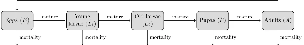
1. Stage-structure. The N. eichhorniae weevil pop-ulation is represented by five development stages (Fig. 1), while the water hyacinth population is con-sidered at its mature stage to examine the influence of the weevils on an established water hyacinth pop-ulation. Individuals in the weevil population enter a stage by developing from the previous stage or by reproduction from the mature stage and leave a stage through death or maturation. By adding stage-structure, the model accounts for more bio-logical detail of the weevils and allows for the ex-plicit modelling of processes pertaining only to spe-cific development stages, making it a more realistic representation. The number of equations necessary to represent the weevil population is limited to the number of development stages that have density-dependent processes. In this paper, similar to the temporal model developed by Wilson [21], the two larval stages and the adult stage are considered suf-ficient to represent the weevil population.
2. Plant growth. Several factors affecting the growth of the water hyacinth are not included in the model as
Eggs (E) Young
larvae (L1)
Old larvae
(L2) Pupae (P) Adults (A)
mature mature mature mature
mortality mortality mortality mortality mortality
reproduce
it is difficult to quantify. These factors include frost, diseases, saltiness of water, wind, humidity, water currents, floods, light and carbon dioxide concen-tration [12, 21]. Constant nitrogen and phosphorus levels are assumed throughout the study.
3. Damage factor. While both theN. eichhorniae lar-vae and adults feed on water hyacinth, it is assumed that only the old larvae cause actual damage to the plant. In addition to the removal of biomass, tun-nelling of larvae into the petioles and the crown of the plant can cause nutrient deficiency as well as provide a route of entry for disease-causing micro-organisms. The movement of larvae between leaves and the crown of the plant may also lead to flood-ing of larval tunnels and a reduction in plant buoy-ancy [21]. Feeding by adults on the outside of the leaves does not directly affect the rhizome or the meristem of the plant, both of which may be dam-aged by larval feeding. In most cases, adult feeding appears to be much less destructive to water hy-acinth and is thought to be negligible compared to damage caused by old larvae [4, 21].
4. Ovipositing. Adult weevils are assumed to start lay-ing eggs immediately after they enter the system and continue to oviposit at a constant rate through-out their lifetime. The oviposition rate is adjusted accordingly to allow females to lay the approxim-ated maximum amount of eggs during their lifetime.
5. Reproduction. When adult density within a con-sidered area decreases below a minimum threshold, it is assumed that they will not be able to reproduce any longer. There has to be a sufficient number of adults within a reachable range of each other for reproduction to occur.
6. Density dependence. From experiments and per-sonal observations, Wilson [21] found it reasonable to assume that due to adult weevil mobility, the fe-male weevils will oviposit regardless of density, res-ulting in density-independent oviposition and egg survival rates for any realistic density of adults per plant. Due to the relative mobility of old larvae, the through-stage survival rates of the old larval and pupal stages of the weevil’s life cycle are also assumed unaffected by density. Density-dependent mortality is only added to the young larval popula-tion as Wilson [21] found that most density depend-ence occurs before damage is caused to the plant. At high larval densities, young larvae may have a higher probability of being stranded in decaying leaves. It is assumed that adults have abundant supplies of any limiting nutrient.
7. Dispersal. The presented spatio-temporal model as-sumes that individuals in the mobile development stages of the weevil population perform an unbiased random walk. This assumption concurs with pre-vious studies which found that weevils randomly disperse throughout a water hyacinth mat without any apparent preference for particular areas of the plants [9]. During each time unit, a proportion of old larvae and adult weevils are assumed to leave their current location to inhabit neighbouring sites within their reach. This motion can be modelled in terms of Fickian diffusion and is approximated by using the Laplacian operator. The water hyacinth dispersal is also described by Fickian diffusion as weed mats randomly expand to neighbouring sites.
8. Domain. For the demonstrative purpose of this study, the spatial domain is assumed to be an isol-ated rectangular water body infested with water hy-acinth to its carrying capacity, surrounded by land use categories considered unsuitable habitat for wa-ter hyacinth orN. eichhorniaeweevils. It is thus as-sumed that neither plant nor weevil enters or exits the domain. The spatial domain is considered het-erogeneous as the plant or weevil densities may vary for different locations due to the fact that weevils are not uniformly spread across an area.
9. Releases. Adult weevils are released by hand from small plastic containers at the accessible edges of an infested water body and take time to disperse to neighbouring sites. In some cases, boats may be used for releases on larger water bodies. Releases are assumed to occur once off or at a constant rate over the period of release. The distribution of the releases may be influenced by the accessibility to the infested area and the number of available BCAs.
2.1 Model formulation and notation Let
W(ξ, t) denote the biomass density of wa-ter hyacinth material (in kg/unit2) at location ξ = [ξ1, ξ2]
T
∈ D at time t, where D is a closed, two-dimensional spatial domain, and E(ξ, t), L1(ξ, t),
L2(ξ, t), P(ξ, t) and A(ξ, t) denote the densities of
bytE. The time spent in each stage of the weevil’s life cycle is temperature-dependent.
In order to model the spatial dynamics of the wa-ter hyacinth and weevil system in a bounded two-dimensional spatial domain, diffusion terms are added to the applicable ordinary delay differential equations in the temporal model presented by Wilson [21]. Let the diffusion coefficientsdW,dL2(θ) and dA be a meas-ure of how effectively water hyacinth, old larvae and adult weevils disperse between neighbouring locations, respectively, invariant in time and space. In addition, an Allee-effect and a term allowing for frequent releases of adult weevils are included, a more detailed temperat-ure dependence is incorporated, as well as slight changes to the modelling of the through stage survival probab-ilities. Furthermore, a different approach towards the modelling of the recruitment and maturation terms for the weevil population is followed and a sufficient expres-sion for the old larval maturation term with dispersal is derived.
LetRi(ξ, t) denote the rate of recruitment into stagei of the weevil’s life cycle at locationξat timet. The rate of recruitment into the young larval stage at location ξ at timetis equal to the number of eggs maturing at the corresponding location and time. The number of eggs maturing is the number of eggs laid at location ξ and tE(θ) days ago – the number of adults present at that location tE(θ) days ago multiplied by the oviposition rate – multiplied by the probability of surviving through the egg stage. The young larval recruitment rate is lim-ited by an Allee-effect, resulting in a decrease of the young larval population growth rate at low adult weevil densities. Once the adult population within a considered area of 1 m2 falls below the minimum threshold for
re-production, a, the negative instantaneous growth rate of the young larvae leads to the extinction of the pop-ulation. The Allee-effect may cause slower spread and decreased establishment likelihood of BCAs, influencing the efficacy and cost of biological control. Expected spa-tial ranges, distributions and patterns of species may be altered when an Allee-effect is present [19], making this an important effect to consider. The rate of maturation out of the young larval stage at location ξ at time t, which is equal to the recruitment rate into the old larval stage at locationξ at timet, is simply the recruitment rate into the young larval stage at timet−tL1(θ) multi-plied by the probability of surviving through the young larval stage. The same logic is followed for the recruit-ment and maturation rates of the other weevil develop-ment stages, except for the maturation rate out of the old larval stage where diffusion is involved. The time-delay term for this rate of maturation must be derived in a different way because an old larva can move during the period between entering the system and maturing
to the next stage and is therefore expected to enter the pupal stage at a point in space different from where it originally emerged. The recruitment rates used in the model are given by
RL1
ξ, t=q(θ)Aξ, t−tE(θ)
σE(θ)
A
ξ, t−tE(θ)
−a
Aξ, t−tE(θ)
, (1)
RL2
ξ, t
=
RL1
ξ, t−tL1(θ)
SL1
ξ, t
if
RL1ξ, t−tL1(θ)>0,
0 otherwise,
(2)
RP
ξ, t
= ¯RL2
ξ, t
σL2(θ), (3)
RA
ξ, t=RP
ξ, t−tP(θ)
σP(θ), (4)
where θ denotes the temperature (in ◦C), q(θ) the rate of oviposition of viable eggs at temperature θ, ti(θ) the development duration in days of stageiof the weevil’s life cycle at temperatureθandσi(θ) the density-independent through stage survival probability for stage i at temperature θ. The calculated development dura-tions of immature stages at different temperatures are given in Table 1.
Table 1: Development duration of weevil life stages, measured at different temperatures.
Development duration (in days)
Temp (◦C) Eggs
(tE)
Young larvae
(tL1)
Old larvae
(tL2)
Pupae
(tP)
16.00 44.00 47.00 35.00 33.00 20.00 24.00 47.00 25.87 29.85 25.00 12.00 28.85 14.42 19.90 30.00 8.00 20.00 10.00 14.93 35.00 16.00 40.00 20.00 29.85 39.00 44.00 47.00 35.00 33.00
Provided the maximum probability of surviving through stagei, attained from Wilson [21], the change in the survival probabilitiesσi(θ) as a result of changes in temperature was determined and is shown in Figure 2.
10 15 20 25 30 35 40
0 0.2 0.4 0.6 0.8 1
Temperature
Surviv
al
probabilit
y E
L1
L2 P
The reaction-diffusion model for the interacting spe-cies, formulated as a system of coupled delay partial dif-ferential equations (PDEs), linked to the set of algebraic equations (1) – (4), is given by
∂W(ξ, t)
∂t =dW∇
2W(ξ, t) +r(θ)W(ξ, t)
1−W(ξ, t)
K
−cL2(θ)L2(ξ, t)
W(ξ, t)
W(ξ, t) +H !
,
(5)
∂L1(ξ, t)
∂t =RL1
ξ, t− µL1(θ) + JL1
W(ξ, t)L1(ξ, t) !
L1(ξ, t)
−RL2ξ, t,
(6)
∂L2(ξ, t)
∂t =dL2(θ)∇
2L 2
ξ, t
+RL2
ξ, t
−µL2(θ)L2(ξ, t)
−RP
ξ, t,
(7)
∂A(ξ, t)
∂t =dA∇
2A
ξ, t+RAξ, t−µA(θ)Aξ, t
+IX
ξ, t
,
(8)
∂SL1(ξ, t) ∂t =SL1
ξ, tJL1 L1(ξ, t−tL1(θ)) W(ξ, t−tL1(θ))−
L1(ξ, t)
W(ξ, t) !
, (9)
where ∇2 ≡ ∂2 ∂ξ12 +
∂2
∂ξ22 denotes the Laplacian oper-ator for diffusion, r(θ) the daily intrinsic growth rate of the plant at temperature θ and K the carrying ca-pacity (kg/unit2) of the water resource. Furthermore, cL2(θ) denotes the rate of damage caused by the older larvae at temperature θ and H the plant density at which herbivore feeding is reduced by half. Paramet-ers q(θ), r(θ), K, cL2(θ), H and JL1 were obtained from Wilson [21].
Assuming a given young larva competes equally with all other young larvae for limited resources, Gurney et al. [8] suggested to reflect this limitation by choos-ing a per capita young larval death rate which var-ies linearly with young larval population. In line with Wilson’s application of this modelling approach [21], the young larval density-dependent mortality rate is given by JL1
W(ξ,t)L1(ξ, t), where JL1 denotes the density-dependent scaling parameter for young larvae which is equal to the number of kilogrammes of plant material per young larva at which the young larval population growth rate is zero. In equations (6) – (8), µi(θ) de-notes the daily density-independent mortality rate for stage i (i = L1, L2 or A) of the weevil’s life cycle at
temperatureθ and is given by
µi(θ) =
−ln(σi(θ))
ti(θ) if σi(θ)>0
1 otherwise.
Finally, I denotes the number of new adult weevils released per location at any time and
X(ξ, t) =
1 if BCAs are released at location ξ
at time t
0 otherwise.
(10)
Since the state variablesW(ξ, t), L1(ξ, t), L2(ξ, t) and
A(ξ, t) represent population densities, they are set to be non-negative real numbers for obvious reasons. The density-dependent survival rate,SL1(ξ, t), is assumed to have a lower bound of zero and an upper bound equal to the density-independent through stage survival rate for young larvae,σL1(θ).
Based on Gourley & Kuang’s [5] formulation of a bounded one-dimensional single-species diffusive-delay population model, the time-delayed maturation term for the old larval stage where there is diffusion is derived for the model in a closed, two-dimensional spatial domainD with homogeneous Neumann boundary conditions. For simplicity’s sake, studies in literature only demonstrate the derivation of the delay term for a one-dimensional domain [5, 7], only mentioning that it should be pos-sible to carry out numerical simulations in higher space dimensions.
In algebraic equation (3), the weighted average ofRL2 at an earlier time is given by
¯
RL2 ξ, t
=
Z
D
G ξ, x, tL2(θ)
RL2(x, t−tL2(θ)) dx, (11)
wherexis another point in space. Old larvae will have emerged at various locations (x) in domainDand may have moved around, being at point ξ on maturing to the pupal stage. The quantity ¯RL2 ξ, tσL2(θ) gives the rate at which old larvae mature into the pupal stage at location ξ and time t, having taken tL2(θ) days to mature. The spatial averaging functionG(ξ, x, t) is the solution of
∂G
∂t = dL2(θ)∇
2
G, (12)
subject to homogeneous Neumann boundary conditions and initial conditions given by
G(ξ, x,0) = δ(ξ−x), (13)
where δ is the Dirac delta function and ∇2 the
Lapla-cian computed with respect to the first argument of G(ξ, x, t). The Dirac delta function, δ(ξ−x), has the value 0 for all ξ 6= x and 1 for ξ = x. Furthermore, function G(ξ, x, t) > 0 for all t > 0. If RL2 ξ, s
≥ 0 for all ξ ∈ D and s ≤ t, then ¯RL2 ξ, t
According to Gourley & Kuang [6], the existence of solutions to one-dimensional delay reaction-diffusion systems, similar to the one described in equations (5) – (9), which is already more complex due to being in two dimensions, have yet to be established. It is therefore as-sumed that a solution to the presented model exists and the focus in the rest of the thesis is turned towards how the model may be applied to optimise water hyacinth biological control release strategies.
A limitation of the time-delayed modelling approach is that time lags allow weevil populations to still exist for a period of time at a specific location after the plant has been driven to extinction at that point in space, as density dependence in terms of limiting resources is only added to the young larval stage. There is a delayed dens-ity dependence effect on the other weevil development stages. In the long term, these delayed effects become negligible and the model still succeeds in providing good estimates of the overall population dynamics.
2.1.1 Boundary conditions Since water hyacinth cannot exist on land andN. eichhorniaeweevils are host-specific BCAs, only able to survive on water hyacinth, it is assumed that neither plant nor weevil enters or exits the domain. System (5) – (9) is therefore subject to homogeneous Neumann boundary conditions given by
n·(D⊗ ∇u) = 0, ∀ξ∈∂D, (14)
wherenis the outward normal vector on the boundary,
Dthe diffusion coefficient matrix, uthe solution of the system and∂Dthe boundary ofD.
2.1.2 Initial conditions Initially the water hy-acinth density is assumed to be at carrying capacity (K = 70 kg/m2) throughout the whole domain under
consideration (D) and all weevil stages are assumed ab-sent prior to BCA releases. A certain amount of adult weevils will be released at specific locations at the edges of the domain at time t= 0. The initial conditions for system (5) – (9) are thus given by
W(ξ, t) = K, for t≤0, ∀ξ∈ D
L1(ξ, t) = 0, for t≤0, ∀ξ∈ D
L2(ξ, t) = 0, for t≤0, ∀ξ∈ D
A(ξ, t) = 0, for t <0, ∀ξ∈ D
A(ξ,0) =
I if X(ξ,0) = 1 0 otherwise
SL1(ξ, t) = σL1(θ), for t≤0, ∀ξ∈ D,
(15)
whereK, I and σL1(θ) are assumed to be positive real numbers.
3
Software implementation
The model was implemented inMatlab9.0 (R2016a) where the system of coupled delay PDEs in a bounded
two-dimensional spatial domain is solved using tools from the PDE toolbox and its built-in functions [20]. Various difficulties encountered during the implementa-tion process are discussed below.
1. System formulation. Firstly, the equations had to be put in the correct form in order to be able to use tools fromMatlab’s PDE toolbox to solve the sys-tem of PDEs, since the toolbox does not have the option for solving nonlinear parabolic PDEs. For each equation, the linear part is put on the left-hand side and the nonlinear part on the right-left-hand side of the equation. Similar to an approach used by Howard [11], the nonlinearity is taken as a driving term from the previous time step and the remain-ing linear equations are decoupled so that 5 sremain-ingle equations are solved rather than a system. Provided the initial conditions, solution times, boundary con-ditions, mesh parameters and various PDE coef-ficients, the built-in parabolic function produces the solution to thefinite element method1 formula-tion of the PDE problem. Theparabolicfunction creates finite element matrices corresponding to the problem internally and callsode15sto solve the res-ulting system of ordinary differential equations.
2. Time lags. Since the built-in functions do not allow for time lags, history matrices containing the solu-tions to the system at all previous time increments are constructed to determine the partial derivative of a function where the solution at a certain time depends on the values of the function at previous times.
3. Spatial averaging. Spatial averaging for the old lar-vae stage, involving both time delay and diffusion, had to be implemented. An explicit expression for the spatial averaging kernelG ξ, x, tL2(θ)
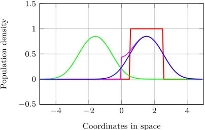
in equa-tion (11) in the bounded two-dimensional case does not exist. Therefore, the expression for the spatial averaging kernel for theunbounded case is used in the implementation and the effect of each reflecting boundary (homogeneous Neumann boundary con-ditions) is accounted for manually. Following an approach used by Powell [16], the effect of reflecting boundaries are simulated by creating artificial pop-ulations of dispersers on the outsides of the bound-aries, which, when they disperse back toward the original grid, will add to the original population the individuals that “reflected” from the bound-aries. This is accomplished by first reflecting the
data of the original grid over each boundary, storing the reflections together with the original grid (nine grids in total) in an artificial grid and considering the new grid as an infinite domain. Spatial aver-aging is then performed over the entire new grid. Finally, the original grid is extracted to obtain the population of interest. The effect of what happens at each boundary of the original grid is illustrated in Figure 3, with a reflecting boundary at 0. The red line resembles the initial population at time 0, blue the dispersal of the original population after a certain time period, green the dispersal of the re-flected population and magenta the final population of interest, which is the population after dispersal, taking the reflecting boundaries into account. The final population distribution (magenta) is the sum of the original (blue) and reflected (green) popula-tion densities for each locapopula-tion within the original grid.
−4 −2 0 2 4
−0.5 0 0.5 1 1.5
Coordinates in space
P
opulation
densit
y
Figure 3: Illustration of how the effect of a reflecting boundary is accounted for in the model.
The recruitment rate RL2(x, t−tL2(θ)) is con-sidered as the initial population for the old larval stage. The individuals disperse randomly accord-ing to the distribution g. Derived from the one-dimensional unbounded expression provided in [5, 6] and similar to an expression used by [16], the spatial averaging Gaussian kernelgfor the two-dimensional unbounded case is given by
g(ξ, tL2(θ)) =
1 4πdL2tL2(θ)
e−(ξ21+ξ22)/4dL2tL2(θ), (16)
with parameters as defined in§2.1. The final pop-ulation distribution aftertL2(θ) days is given by
R∞ −∞
R∞
−∞g(ξ, x, tL2(θ))RL2(x, t−tL2(θ)) dx
=RL2(ξ, t−tL2(θ))∗g(ξ, tL2(θ)),
(17)
where the latter operation is called the convolution. Algorithm 1 describes the spatial averaging process.
4. Frequent releases. Implementing frequent releases for the spatially explicit domain proved to be more
Algorithm 1: Spatial averaging for old larval stage
Input : Distribution ofL2 as they enter the stage at an earlier time, mesh coefficients, development duration ofL2 stage,L2diffusion rate.
Output: Distribution ofL2 ready to mature at current time.
Create two-dimensionala×bgrid of geometry;
1
Create triangular mesh of grid;
2
SetRL2(i, t−tL2(θ)) as initial population for each 3
nodeiof the grid;
Define expressionggiven in Eq. (16) for spatial
4
averaging kernel over entire mesh;
Normalise kernel using the built-intrapzfunction;
5
// g/trapz(trapz(g))
Perform Fast Fourier Transform of gin two
6
dimensions for convolution in Eq. (17); // fft2(g)
Create reflections of the original grid data over each
7
boundary;
Store the reflected grids together with the original grid
8
in a new 3a×3bgrid in their corresponding positions; Perform dispersal on the entire 3a×3bgrid;
9
Extract the original grid’s data;
10
0 50 100
Positionξ1 Positionξ2
Adult
densit
y
(/m
2)
(a) To the centre of the domain.
0 50 100
Positionξ1 Positionξ2
Adult
densit
y
(/m
2)
(b) First to the right of every point.
Figure 4: The two options for the direction in which searches for feasible points of release may be conducted when frequent releases are involved.
points of release. Since there was not a significant difference in the outcome between the two search options, the search straight to the centre of the do-main was implemented in the interest of multiple releases per edge, where BCAs are already distrib-uted along an edge and releases to the sides of the original positions become redundant. In the main algorithm where the system of PDEs is solved (Al-gorithm 2), a release is implemented as an addition ofIto the right-hand side of the adult weevil popu-lation equation if both the required constraints are met at the considered time and location.
In light of these difficulties, let equations (5) – (9), governing the change inW(ξ, t), L1(ξ, t), L2(ξ, t), A(ξ, t)
andSL1(ξ, t), respectively, be the five PDEs being solved in the main procedure (Algorithm 2), assuming para-meters and variables as defined in§2.1. Let Unbe the history matrix for the time-dependent results of thenth
PDE.
The water hyacinth and weevil system incorporates variable temperature. Algorithm 3 gives more insight into the process being carried out when the TempDep function is called in lines 6 and 13 of the main algorithm. The temperature-dependent parameters used in sys-tem (5) – (9) arer(θ),cL2(θ), q(θ), dL2(θ),tE(θ), tL1(θ), tL2(θ), tP(θ), σE(θ), σL1(θ), σL2(θ), σP(θ), µL1(θ), µL2(θ) and µA(θ). As described in Algorithm 3, the values of these parameters are updated at the beginning of each month when a new average temperature is set.
Algorithm 2: Solving the system of PDEs
Input : Total running time, starting month, magnitude of releases, release frequency, points of release, Allee-effect threshold, initial conditions.
Output: Solutions to the PDEs at every node for every time increment.
Create two-dimensional grid of geometry;
1
Assign boundary conditions given in Eq. (14) to edges;
2
Create triangular mesh withmnodes;
3
Create time vector withM time-stepping increments;
4
Assign constant values toKandJL1used in Eqs. (5)–(9);
5
Call temperature-dependent parameter values for starting
6
month; // TempDep(month,1)
fori←1tomdo 7
Set initial conditions given in (15) for Eqs. (5)–(9);
8 end 9
Set initial conditions as first column of eachUn;
10
fort←1toM do 11
if time increment a multiple of 30then 12
Update temp. dependent parameter values for
13
new month; // TempDep(month,t)
end 14
if (t−tE(θ)−tL1(θ)−tL2(θ))>0then 15
Perform spatial averaging forL2; // Alg. 1
16
end 17
if time increment a multiple of frequencyf then 18
Allow additions to adult populationAat timet 19
(1stprocedure for Eq. (10));
end 20
Determine coordinates for additions to adult
21
populationA(2ndprocedure for Eq. (10));
fori←1tomdo 22
Determine nonlinear interactions forW using
23
Eq. (5);
if (t−tE(θ))>0thencalculateRL1(i, t) using 24
Eq. (1);
elseRL1(i, t) = 0;
25
if (t−tE(θ)−tL1(θ))>0 & RL1(i, t−tL1(θ))>0
26
thencalculateRL2(i, t) using Eq. (2);
elseRL2(i, t) = 0; 27
if (t−tE(θ)−tL1(θ)−tL2(θ))>0thencalculate
28
RP(i, t) using Eq. (3);
elseRP(i, t) = 0;
29
if (t−tE(θ))>0thendetermine nonlinear
30
interactions forL1 using Eq. (6);
elsenonlinear interactions forL1= 0;
31
if (t−tE(θ)−tL1(θ))>0thendetermine
32
nonlinear interactions forL2 using Eq. (7);
elsenonlinear interactions forL2= 0;
33
if (t−tE(θ)−tL1(θ)−tL2(θ)−tP(θ))>0then 34
determine nonlinear interactions forAusing Eq. (8);
elsenonlinear interactions forA= 0;
35
if (t−tE(θ)−tL1(θ))>0thendetermine
36
nonlinear interactions forSL1 using Eq. (9); elsenonlinear interactions forSL1= 0;
37
end 38
Define nonlinear interaction terms for allnPDEs at
39
centerpoints of mesh triangles by interpolation using the built-inpdeintrpfunction;
Solve allnPDEs withparabolicfunction;
40
Setzero as a lower bound for all solutions;
41
Append new solutions to eachUnfor allnPDEs;
Algorithm 3: Temperature-dependent parameters
Input : Starting month, time increments.
Output: Temperature-dependent parameter values, linear interactions and diffusion coefficients. Set vector with monthly average temperatures,
1
depending on starting month;
if first time increment then // t==1
2
Set average temperatureθfor first month;
3
Calculate temp. dependent parameter values;
4
Calculate temp. dependent linear interactions for
5
Eqs. (5)–(9);
Calculate temp. dependent diffusion coefficients
6
for Eqs. (5)–(9);
else if time increment a multiple of 30 then
7
// mod(t,30)==0
Update average temperatureθfor new month;
8
Calculate temp. dependent parameter values;
9
Calculate temp. dependent linear interactions for
10
Eqs. (5)–(9);
Calculate temp. dependent diffusion coefficients
11
for Eqs. (5)–(9);
end
12
4
Model calibration and testing
In§4.1 and§4.2, suitable parameter values for the dif-fusion coefficients for adult weevils and water hyacinth, respectively, are determined by means of reverse engin-eering.
4.1 Adult weevil dispersal By means of dispersal experiments, Haag [9] determined that even in the ab-sence of flight muscles, adult weevils are able to move between adjacent plants over a distance of at least 4 m in a course of one month. Information about adult move-ment over longer distances is still lacking. It is therefore assumed that adult weevils travel a maximum distance of 4 m per month. By means of reverse engineering, a diffusion coefficient ofdA= 0.09 m2/day was obtained. In Figure 5, the dispersal of adult weevils released within a 1 m2area at the edge of an infested water body at time
0, withdA= 0.09 m2/day, is shown as obtained from the
simulation output.
4.2 Water hyacinth population growth Literat-ure indicates that the water hyacinth surface area may increase by an average of 8% per day under good growing conditions [12]. A diffusion coefficient of dW = 0.08 m2/day reflects this assumed daily surface
expansion. Figure 6 illustrates the population growth of the weed with the obtained diffusion rate without the influence of the BCAs. The red line indicates the car-rying capacity of the water body. Once the plant dens-ity at a certain location reaches the carrying capacdens-ity,
0 10 20 30
0 5 10
Positionξ1(m)
P
osition ξ2
(m)
(a) Initial population.
4m
0 10 20 30
0 5 10
Positionξ1(m)
P
osition ξ2
(m)
(b) Dispersal after one month.
Figure 5: Adult weevil dispersal over one month with the derived diffusion coefficient ofdA = 0.09 m2/day.
0 10 20 30
0 20 40 60 80
Positionξ1(m)
Plan
t
densit
y
(kg/m
2)
(a) Initial population.
0 10 20 30
0 20 40 60 80
Positionξ1(m)
Plan
t
densit
y
(kg/m
2)
(b) After eight weeks.
Figure 6: Water hyacinth population growth over eight weeks without BCA releases.
5
Model validation
Conceptual model validation may be described as the process of proving that the theories and assumptions un-derlying a model yields results within a sufficient range of accuracy, and that the model representation of the real-life problem is sufficient in accordance with the in-tended purpose of the model. A number of validation techniques exists of which degenerate tests and face val-idation are used in this paper [17]. A series of degener-ate tests were performed to determine whether changes in certain parameter values yield the expected outcome. The effect of different magnitudes of adult releases, tem-peratures, and release frequencies on controlling water hyacinth are demonstrated in this section. The results from these tests were also compared to experiences in practice, thereby performing face validation. In addi-tion to conceptual validaaddi-tion, these tests demonstrate how the model may be used as a decision-making tool for BCA release strategies.
5.1 Effect of different magnitudes of adult re-leases As a result of more BCAs being present to cause damage, an increase in the magnitude of a release (I) is expected to result in a faster decrease in initial plant density in the short term. For high levels ofI, however, density dependence in the young larval stage is expected to result in a faster decrease in weevil population dens-ities compared to lower values ofI. In time, decreases in the weevil populations will result in increases in the plant population densities again.
Figure 7 shows the effect of different magnitudes of N. eichhorniae adult weevil releases on the total pop-ulation densities of water hyacinth and the various life stages of the weevil over three months. For both sim-ulations, the applicable number of adults was released in January at the four edges of a 10 m ×10 m area in-fested with water hyacinth. Young larvae (L1) appear
tE(θ) days after adult releases and damage-causing old larvae (L2)tE(θ) +tL1(θ) days after initial releases. As the total water hyacinth population decreases due to old larval feeding, density dependence causes a decrease in both larval populations, giving the plant time to increase before the next generation of damaging larvae appear. As expected, model output suggests that releases of 200 weevils at the edges at time 0 will have a greater effect on the total water hyacinth population over a period of three months. Model output also reflects the discern-ible decreases in water hyacinth populations that were observed after about 70 days in comparable real life re-lease scenarios [3].
The long term plant and weevil densities responses are more variable due to populations being exposed to density-dependent interactions for a longer period of
0 30 60 90
0 3000 6000 9000 12000
t (days)
Plan
t
(kg)
&
w
eevil
densities
(/100
m
2)
W L1 L2 A
(a) 100 adults released at each edge.
0 30 60 90
0 3000 6000 9000 12000
t (days)
Plan
t
(kg)
&
w
eevil
densities
(/100
m
2)
W L1 L2 A
(b) 200 adults released at each edge.
Figure 7: The change in the total plant (W), young larval (L1), old larval (L2) and adult (A) population
densities over three months for different magnitudes of BCA releases.
time, as expected. The model correctly reflects the hy-dra effect where an increase in the number of BCAs re-leased does not always result in lower average plant dens-ity in the long term due to a greater impact of densdens-ity dependence on the larval stages when more BCAs are released, yielding less damage-causing old larvae to sup-press weed densities.
de-crease fast once old larvae enter the system. Due to density dependence, this should in time result in faster decreases in weevil populations, yielding greater oscilla-tions of population densities.
Simulations were performed to investigate the effect on water hyacinth populations in the Cape Town re-gion when adult weevils are released once-off in summer (December, with an average high temperature of 25◦C) or winter (June, with an average high temperature of 18◦C), subject to monthly varying temperatures. Once-off releases of 1 000 BCAs at time t = 0 at each of the four edges of a 30 m × 30 m infested water body were simulated. Figure 8 illustrate the change in total plant density over six months for summer and winter releases, respectively. It may be seen that the delay between subsequent damage-causing old larval genera-tions gives the weed a chance to grow back. Six months later, the BCAs that were released during summer are exposed to colder winter temperatures, but favourable weather conditions during the first months after releases supported establishment and BCAs could still contrib-ute towards the suppression of weed populations during subsequent colder seasons. Confirming what happens in practice, results (Fig. 8) indicate that BCAs may not be able to establish under certain temperature thresholds due to slower development and higher mortality.
0 30 60 90 120 150 180 45000
50000 55000 60000 65000
t (days)
T
otal
plan
t
densit
y
(kg/900
m
2)
(a) Summer release.
0 30 60 90 120 150 180 45000
50000 55000 60000 65000
t (days)
T
otal
plan
t
densit
y
(kg/900
m
2)
(b) Winter release.
Figure 8: The change in the total plant density over a time period of six months after once-off releases of 1 000 BCAs at four edges in December (a) and June (b).
5.3 Effect of different release frequencies on the control of water hyacinth A direct relationship between the frequencyf of BCA releases and the adult weevil population densities is expected. In order to test whether the implementation of the frequent BCA release process responds correctly, simulations were performed with once-off, weekly, two-weekly and four-weekly re-leases, respectively, with a magnitude of 100 adult weevils per release at each of the four edges of the con-sidered domain and with temperature held constant at 30◦C over a period of one year.
As expected, model responses indicate a decrease in the average plant population density over time when BCAs are released more often. In Figure 9, the plant and adult population densities, subject to once-off (f = 0), low frequency (f = 28) and high frequency (f = 7) re-leases over the period of one year, are shown. Water hyacinth populations are suppressed faster the more of-ten adult weevils are released, as expected. The model succeeds to accurately reflect the regrowth of the weed after a period of time, subsequent to being suppressed to very low densities over the entire domain. Frequent adult weevil releases are ceased once the weed is sup-pressed below a certain threshold and resumed when the weed grows back to sufficient densities for releases. As expected, higher frequencies of releases result in more effective weed suppressions after regrowth.
6
Conclusion
A two-dimensional reaction-diffusion model, formu-lated as a system of coupled PDEs, was presented in order to describe the population growth and dispersal of water hyacinth and the interacting populations of the development stages of theN. eichhorniaeweevil as BCA in a temporally and spatially variable environment. Nu-merical solutions to the system of PDEs in a bounded domain with homogeneous Neumann boundary condi-tions were obtained by means of simulacondi-tions of the finite element method implemented inMatlab. Various chal-lenges in implementing time delays, spatial averaging, frequent releases and fluctuating temperatures were dis-cussed.
repres-0 100 200 300 0
3500 7000
t (days)
Plan
t
densit
y
(kg/100
m
2)
(a) Plant densities withf= 0.
0 100 200 300
0 2000 4000
t (days)
Adult
densit
y
(/100
m
2)
(b) Adult densities withf= 0.
0 100 200 300
0 3500 7000
t (days)
Plan
t
densit
y
(kg/100
m
2)
(c) Plant densities withf= 28.
0 100 200 300
0 2000 4000
t (days)
Adult
densit
y
(/100
m
2)
(d) Adult densities withf= 28.
0 100 200 300
0 3500 7000
t (days)
Plan
t
densit
y
(kg/100
m
2)
(e) Plant densities withf= 7.
0 100 200 300
0 2000 4000 6000
t (days)
Adult
densit
y
(/100
m
2)
(f) Adult densities withf= 7.
Figure 9: Plant and adult population densities for once-off (f = 0), low frequency (f = 28) and high frequency (f = 7) releases over a time period of one year.
entation of the population growth and dispersal of the interacting species, the model may be used to provide guidance towards the optimal magnitude, frequency, sea-sonal timing and distribution of BCAs releases.
Acknowledgements
We thank Sisanda Nuse from Invasive Species Man-agement who provided insight and information that greatly assisted the research, although she may not ne-cessarily agree with all of the interpretations of this pa-per. A special thank you to the anonymous reviewers whose insightful feedback notably improved the manu-script.
References
[1] Al-Omari, J.F.M. & Gourley, S.A. 2005. A non-local reaction-diffusion model for a single species
with stage structure and distributed maturation delay. European Journal of Applied Mathematics. 16(1): 37–51.
[2] Byrne, M., Hill, M., Robertson, M., King, A., Katembo, N., Wilson, J., Brudvig, R., Fisher, J. & Jadhav, A. 2010. Integrated management of water hyacinth in South Africa. WRC Report. (454/10).
[3] Conlong, D.E. 2014. Senior Entomologist at South African Sugarcane Research Institute, Mount Edge-combe, [Personal Communication]. Contactable at [email protected].
[5] Gourley, S.A. & Kuang, Y. 2003. Wavefronts and global stability in a time-delayed population model with stage structure. Proceedings of the Royal So-ciety of London Series A: Mathematical, Physical and Engineering Sciences. 459(2034): 1563–1579.
[6] Gourley, S.A. & Kuang, Y. 2004. A delay reaction-diffusion model of the spread of bacteriophage in-fection. SIAM Journal on Applied Mathematics. 65(2): 550–566.
[7] Gourley, S.A., So, J.W.H. & Wu, J.H. 2004. Non-locality of reaction-diffusion equations induced by delay: biological modeling and nonlinear dynamics. Journal of Mathematical Sciences. 124(4): 5119– 5153.
[8] Gurney, W.S.C., Nisbet, R.M. & Lawton, J.H. 1983. The systematic formulation of tractable single-species population models incorporating age structure. The Journal of Animal Ecology. 52(2): 479–495.
[9] Haag, K.H. 1986. Effects of herbicide application on mortality and dispersive behavior of the wa-ter hyacinth weevils, Neochetina eichhorniae and Neochetina bruchi (Coleoptera: Curculionidae). Environmental entomology. 15(6): 1192–1198.
[10] Hill, M.P. & Olckers, T. 2001. Biological control initiatives against water hyacinth in South Africa: constraining factors, success and new courses of action. Proceedings of the Second Meeting of the Global Working Group for the Biological and In-tegrated Control of Water Hyacinth. Beijing, China, ACIAR proceedings No. 102. 33–38.
[11] Howard, P. 2005. Partial differential equations in
Matlab7.0. University of Maryland, College Park
(MD).
[12] Jones, R.W. 2009. The impact on biodiversity, and integrated control, of water hyacinth,
Eich-hornia crassipes (Martius) Solms-Laubach (Ponte-deriaceae) on the Lake Nsezi - Nseleni River Sys-tem. PhD Dissertation. Rhodes University, Gra-hamstown.
[13] Julien, M.H., Griffiths, M.W. & Wright, A.D. 1999. Biological control of water hyacinth. The weevils Neochetina bruchi and N. eichhorniae: biologies, host ranges, and rearing, releasing and monitoring techniques for biological control of Eichhornia cras-sipes. Australian Centre for International Agricul-tural Research (ACIAR) Monograph No. 60, Can-berra.
[14] Nuse, S. 2015. Consultant at Environmental Re-source Management Department, Invasive Species Management, Westlake, [Personal Communication]. Contactable [email protected].
[15] Penfound, W.T. & Earle, T.T. 1948. The bio-logy of the water hyacinth. Ecological Monographs. 18(4): 447–472.
[16] Powell, J. 2001. Spatio-temporal models in eco-logy: an introduction to integro-difference equa-tions. Utah State University, Logan (UT).
[17] Sargent, R.G. 2013. Verification and validation of simulation models. Journal of Simulation. 7: 12–24.
[18] S¨uli, E. 2012. Lecture notes on finite element meth-ods for partial differential equations. Mathematical Institute, University of Oxford, Oxford.
[19] Taylor, C.M. & Hastings, A. 2005. Allee-effects in biological invasions. Ecology Letters. 8(8): 895–908.
[20] The MathWorks Inc, . Matlab version 9.0 (R2016a). [Computer Software], Natick (MA).