STUDY OF NAVIER – STOKES EQUATION SOLUTION II. THE USE OF LAMINAR SOLUTIONS
Yakubovskiy E.G. e-mail [email protected]
Laminar Solution of Navier – Stokes Equation. Value of round pipeline resistance coeffi cient for arbitrary Reynolds number and roughness degree are known only from experiment. It is proposed, using complex solution, to obtain a solution of Navier – Stokes equations and based on the qualitative reasons to defi ne roughness infl uence on the solution of Navier – Stokes equation. It was possible to draw classical Nikuradze curves for round pipeline resistance coeffi cient versus Reynolds number and roughness degree with an accuracy of 10 %.
Keyword: large dimensionless unknown functions, solutions of non-linear partial differential equation, Navier – Stokes equation, turbulent function, fl uid fl ow resistance coeffi cient, round pipeline
The problem of turbulent fl uid motion de-scription has not been solved yet. It creates diffi culties when oil, gas pipelines design cal-culation is performed. Besides, there are no theoretical methods for description of bodies motion in turbulent environment. These meth-ods would be necessary for description of mo-tion of aircrafts, submarines or above-water ships in the turbulent mode. Without simula-tion of bodies mosimula-tion in wind tunnels or water basins, design of the bodies moving in the vis-cous environment is impossible.
There are approximate formulas for pipe-line resistance coeffi cient at some ranges of Reynolds numbers, see [1, 2]. But they are empirical approximate formulas and they are applicable only for particular Reynolds num-ber ranges.
Classical experimental Nikuradze curves of round pipeline resistance coeffi cient versus Reynolds number and roughness degree are well known. Approximation of convective term reducing Navier – Stokes problem to linear one with effective turbulent viscosity is applied. But such transformation distorts solution of Navier – Stokes equations and for matching to experiment the turbulent viscosity coeffi cient can have any value, up to negative. Galerkin method which brings hydrodynamic problem solution to system of non-linear ordinary dif-ferential equations is applied. But in the case of turbulent mode, this non-linear equation system has complex balance positions, i.e. the solution is complex. Indeed, hydrodynamics equation system, in turbulent mode, in real plane does not have any solutions, the equation solution tends for infi nity, see [3] and main part I of the
paper. But complex solution is fi nite. About physical meaning of the complex solution and oscillatory behavior of its imaginary part see [4, 5] or article III of this paper. Thus, it is nec-essary to solve hydrodynamic problems for turbulent mode in complex plane. At that, the turbulent solution is not single-valued, there are fi nite number of the solution branches.
Calculation of Round Section
Pipeline Resistance Coeffi cient
for Incompressible Fluid
This algorithm has been used for calcula-tion of resistance coeffi cient for pipeline with round cross section. The algorithm is described in article [6] in English. We will seek the solu-tion of problem for cross secsolu-tion round pipeline
in form , in cylindrical
system of coordinates. As external factor acts only along longitudinal axis
where P2, P1 – pressure in initial and fi nal part of the pipeline; L – length of the pipeline, radial and angular velocities components are
neglect-ed. External action is equal to . Ac-cording to formula (6), the pressure gradient is equal to . So we have the equation
Substituting velocity value we obtain
Multiplying this equation by radius and performing integration over radius, as we use cylindrical coordinate system, we have
To obtain fi nite number of solutions we will multiply equation (1a) by function
and integrate over volume. Then we will obtain fi nite number of turbulent solu-tions both for smooth and rough surfaces. Sta-tionary laminar solution satisfying condition
is single-valued as in the equation (1a) the laminar solution is identical for differ-ent values of . At the same time, likewise Schrödinger equation, fi nite number of turbulent solutions is found, each has its own energy. At transition from one state to another, discrete energy is radiated. The own energy minimum value defi nes the solution choice.
After calculating a module of the right part and averaging module of deviation angle tan-gent, we obtain
(1b)
It will be seen that when minus sign is cho-sen for value of average module of deviation angle tangent , roughness presence increases fl ow velocity as the full derivative
increases and this is
not correct, fl ow velocity has to decrease due to roughness presence.
When turbulent viscosity is taken into ac-count, negative value of average velocity asso-ciated with process velocity correlation
func-tion , see [1], is used and
this leads to plus sign for average module of roughness inclination tangent. The movement equation taking into account disturbances is
That is, convection term should be taken with minus, at right part of (1b) should be tak-en with plus.
Besides, it is necessary to choose plus for average module of roughness inclination tangent to obtain complex turbulent solution. Otherwise, solution describing pulse turbulent mode will not be steady.
Changing pipeline radius to diameter and dividing by value , we obtain
(2)
If you use another branch of root mean square unsteady solution and following equa-tion will be obtained
(3)
Thus, steady solution for large difference in pressure is
Laminar solutions of these two equations at small pressure difference are the same. For turbulent mode with big pressure the solution has linear dependence of Reynolds number versus pressure square root. At small pressure increase, Reynolds number also grows and, as it follows from (3), pressure is increased. So the solution is not steady. In case of the com-plex solution it is equal to
At that, when pressure increases, imagi-nary part of velocity increases too and this does not lead to increase of real pressure, the real pressure keeps the value unchanged.
has the molecular nature, it is defi ned by av-erage atom size equal to avav-erage geometrical difference between the nuclear size rA and size of Bohr orbit when the distance be-tween atoms a = 3,043A is equal to some value determined by properties of pipeline boundary, iron, titanium and carbon. Distance between iron atoms is aFe = 2,87A, between titanium atoms – aTi = 3,46A, between carbon atoms – aC = 3,567A, see [7]. At the same time, the absolute value of tangent of micro roughness height inclination for metal surface of the pipe-line is determined by formula
The average tangent of inclination is equal to
In this paper, critical Reynolds number was calculated with respect to radius. Critical Reynolds number with respect to diameter is equal to Rcr = 2300. But why critical Reynolds number for the sphere is equal to 3∙105? This is
due to different defi nition of critical Reynolds number. This value is equal to
where leff – effective hydrodynamic size of the body, including medium, a – true geometrical
body size, and –
molecu-lar tangent of roughness inclination. And the ratio can be equal to .
Critical Reynolds number is equal to Rcr = 2300. Macro-roughness elements
are rarer and this causes increase of resistance coeffi cient at Reynolds numbers which is 12 or more times more.
So we obtained a stationary criterion for Navier – Stokes equations taking into account one term of the solution series for one-dimen-sional case:
For one-dimensional case, on condition of pipeline cross section area constancy, the
con-tinuity equation is the same. Laminar solution of this equation is
For external pressure equal to , a complex solution and turbulent mode take place as Reynolds number from this point is equal to critical value. From experiment and calculation, we have critical Reynolds number for round pipeline
The pipeline resistance coeffi cient for round cross section pipe is determined by for-mula (we substituted to the forfor-mula the pres-sure difference expressed through dimension-less pressure)
The average velocity used for Reynolds number is equal to
The pipeline resistance coeffi cient λlam as-ymptotic for laminar mode in round cross sec-tion pipeline is calculated truly.
Asymptotic behavior of the pipeline resistance coefficient is obtained for small Reynolds numbers when the convective term is small.
Computing more precisely, contribution of rotary imaginary part to forward velocity of fl ow movement corresponds to square root of imaginary part according to formula (4)
(4)
and it is necessary to use value of ratio of Reyn-olds number to square root of dimensionless pressure as value of order 1 in the turbulent mode. At infi nite pressure, Reynolds number for the fl ow is proportional . At that, the smoothest surface is the surface with average module of inclination tangent equal to inverse value of critical Reynolds number. For solution in the form of series, another value of α will be calculated. This value is defi ned from identical values of resistance coeffi cients at large Reynolds numbers and molecular rough-ness. The smoothest surface corresponds to av-erage module of tangent of inclination equal to the inverse value of critical Reynolds number as the smallest modules of tangent of inclina-tion correspond to molecular type of rough-ness. At that, effective diameter is less than true diameter. The average module of tangent of in-clination angle can not be less than molecular roughness and its minimum value is equal to . That is, 1 is the maximum value
of ratio of effective diameter to true diameter because α = 2. For external problem, effective diameter will increase, and the coeffi cient will be determined by formula
Coeffi cient β is proportional to
At zero macro roughness, effective diam-eter is equal to 1, that is, when roughness is increased, effective diameter decreases. Value was obtained from nu-merical experiment that corresponds to fourth root of mean square deviation. At zero macro roughness, micro roughness presents. And ra-tio of tangent of macro inclinara-tion roughness to micro roughness is more than
At l/k = 30, we have value of effective pipeline diameter
At the same time, diameter is changed only for coeffi cient of pulsing part of the solution, i.e. for imaginary part from where the
multi-plier
origi-nates as the imaginary term is proportional to which is averaged. At that, value
corresponds to fourth root of mean
square deviation.
Here, infl uence of walls roughness in tur-bulent fl ow on imaginary part of Reynolds number of the fl ow is taken into account. To obtain curves with constant roughness height, it is necessary to enter effective average mod-ule of tangent of roughness inclination angle. The effective average module of tangent of roughness inclination angle has to depend on
external pressure .
And in points of infi nite Reynolds num-bers or dimensionless pressure, we have the roughness corresponding to constant rough-ness height
where k – mean square root of the roughness height; r0 – radius of round cross section of the pipeline.
The formula is chosen in such a way that it defi nes correctly dependence of Reynolds number versus external pressure and pipeline resistance coeffi cient at infi nite Reynolds num-bers and external pressure
When average module of tangent of roughness inclination angle is constant but roughness
height k is varying we obtain a curve which differs from Nikuradze curve.
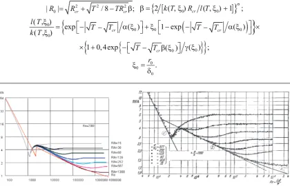
Fig. 1. Curve of round pipeline resistance coeffi cient versus Reynolds number for different mean square root tangent of roughness inclination angle
But Nikuradze formula is obtained for constant ratio of pipeline radius r0 to average rough-ness height k. The formula (4) contains effective average module of tangent of roughrough-ness in-clination angle expressed through ratio of pipeline radius to average roughness height using dimensionless pressure
Value . Infl uence of effective av-erage module of tangent of roughness inclina-tion on fl ow property depends on Reynolds number or pressure difference.
Empirical formula for fi nding of coeffi -cients α(ξ0), β(ξ0), γ(ξ0) is following
At the same time, at the beginning of for-mation of the complex solution imaginary part
, or at the beginning of turbulent solution, roughness inclination tangent is equal to approximately 1, and curves for different roughness inclination tangents coincide.
At that, fl ow resistance coeffi cient for round pipeline is determined by formula
, Reynolds number calculated
based on the average velocity of fl ow
move-ment is equal to . Resistance
coef-fi cient at infi nite pressure is proportional to
. Here we
demon-strate curves for solution obtained using one term of the series.
theoretical curve convective term is taken into account which became equal to zero after aver-aging in laminar mode.
This curve was calculated for constant fl ow temperature over the fl ow cross section
there-fore in case of weak dependence of kinematic viscosity on temperature the formula will not change. For turbulent mode, it is necessary to substitute into the formula normalized pressure and ratio of pipeline radius to roughness height
Fig. 2. Calculated and measured dependence of round pipeline resistance coeffi cient versus Reynolds number for different roughness
And the formula is constructed so that . In case of the laminar mode there is a simple formula for Reynolds number:
Algorithm for Solution of Internal Hydrodynamic Problem for Arbitrary Flow Geometry
Navier – Stokes equations in Cartesian coordinates is
(5)
We will solve a three-dimensional laminar stationary problem without convective term for defi ned external action gl
Let us transform this equations to dimensionless form by dividing it by v2/d3, as a result we
obtain dimensionless equation
We will seek solution of continuity equation for external action, where ri – response to exter-nal action
(6)
From this we obtain equation for fi nding of fl ow pressure
We will seek the pressure value in the form . Then we will substitute
pressure into expression under the integral sign, multiply by φm(y1, y2, y3), and perform integration over the volume, then we obtain a system of linear equation
bm = Amnan. Expressions for coeffi cients are
where hl(y1, y2, y3) is defi ned by external action. Let us transform Navier – Stokes equations to dimensionless form by dividing it by v2/d3, and we have dimensionless equation
Then we multiply Navier – Stokes equations by area of fl ow tube cross section, write the
equa-tions along laminar solution and enter fl ow tube with constant fl ow, see [8]. . In the
convection term and in pressure gradient, we enter the derivative in the direction corresponding to the direction of fl ow lines in laminar solution. When substituting of the solution into equation
(7)
where Ss – fl ow tube cross section in laminar mode, expression Rs[y1(α, β), y2(α, β), y3(α, β)] is a stationary solution of Navier – Stokes equa-tions without convection term which is equal to zero for fl ow tube as it does not depend on longitudinal coordinate.
We built these fl ow tubes for any external action which affects pressure difference. Fur-ther we consider roughness and under certain conditions obtain complex turbulent solution which is associated with infl uence of quadratic convection term with small multiplier, taking into account roughness, which yields complex solution at large pressure difference. At the
same time, we reject real solution which was obtained for another sign of the module of av-erage deviation, as it does not defi ne fl uctuat-ing, turbulent solution. And imaginary part of the solution defi nes the solution pulsations.
If another sign of square root is chosen and correlation function of the process , where is a velocity deviation from its aver-age value, is taken into account, turbulent vis-cosity becomes negative.
Taking roughness into account results in dependence of the pipeline radius a(s) on mac-ro-roughness. Further we will extract the term da/ds associated with roughness and will fi nd average value of its module. At the same time, we will make averaging of the equation with respect to s. It can be found out that convec-tion term in laminar mode for smooth surface is equal to zero, and roughness has to be taken into account for non-zero value. So, we have the equation
To take into account roughness of pipe-line surface and obtain turbulent solution, it is necessary to consider the average module of tangent of roughness inclination angle. Then this convective term will have a small multi-plier, and the convection term will be non-ze-ro. This term is proportional to average value of tangent of module inclination at roughness
. At the same time, there is a term
depending on variable pipeline cross section area . And fl ow lines of complex turbulent solution corresponding to fl ow lines of laminar solution will remain the same but there will be a solution pulsing around laminar fl ow lines. At that, the pulsations are defi ned by imagi-nary part of velocity, and the imagiimagi-nary part of the solution, equal to a constant, means pulsa-tions with amplitude equal to imaginary part of velocity.
Now, we will substitute the solution (7) into Navier – Stokes equations and will in-tegrate along fl ow tubes, will multiply by Rcr in domain where this value meets a condition
and where – average
module of inclination tangent for not remov-able micro roughness with envelope forming macro-roughness, and we will obtain the fol-lowing equation
where Rs(y1, y2, y3), p(y1, y2, y3) are determined from laminar solution and continuity equation, and function of external action hl(y1, y2, y3) is defi ned. So it was found out that micro rough-ness located along all length of the pipeline defi nes critical Reynolds number. This micro roughness is less than macro-roughness which affects resistance coeffi cient at large Reynolds numbers. But as Reynolds number depends on pipeline geometry through its diameter, then critical Reynolds number is inversely propor-tional to the average module of tangent of mi-cro roughness inclination and depends on pipe-line geometry. At the same time, reduction of pipeline radius results in negative da/ds value and, therefore, absence of complex turbulent solution in the narrow place, i.e. the critical Reynolds number raises. On the contrary, the pipeline widening causes increase of da/ds and, therefore, reduction of critical Reynolds number and can result in earlier occurrence of complex solution, i.e. the turbulent mode.
And, as Reynolds number depends on tem-perature through dependence of kinematic vis-cosity on temperature, it is obvious that occur-rence of critical Reynolds number depends on environment temperature.
Coordinates of balance position are defi ned from a quadratic equation
In this case, turbulent formula for roughness calculation is applicable due to identical averag-ing method in turbulent mode
where – effective average
tangent of roughness inclination, ξ0 – ratio of roughness height to pipeline radius and critical Reynolds number is value of Reynolds number corresponding to the beginning of the complex solution. At the same time, for small Reynolds number we obtain a laminar solution. But diffi culties in obtaining of turbulent solu-tion do not come to an end. It is necessary to
de-fi ne effect of the surface roughness and for this use of experimental data is still inevitable. In principle, exact dependence of Reynolds num-ber for smooth surface on macro-roughness is necessary to be learned. But external problem has some features associated with existence of resistance crisis which is caused by presence of a trace behind the body placed into the fl ow. This trace does not present in internal problems such as fl ow in pipeline.
Specifi city
of Flow Velocity Calculation for Sphere
Let us fi nd out solution of Navier – Stokes equations for external problem. We have lami-nar solution for sphere motion in fl uid for small Reynolds number. It yields the following ve-locity distribution, see [8]:
At that, pressure dependence on fl ow pa-rameters is
Motion equations in spherical coordinate system for solutions which do not depend on angle φ can be written as
Let us change coordinate system to ξ, τ, θ with unknown Rr, Rθ, P, the coordinate system is
defi ned by formula , after division of the equation system by
At that, in dimensionless constants, solution can be expressed as
But if you consider solution for one domain θ [0, π], zero value will be obtained for
coef-fi cient Rx. So, the domain should be divided into two parts θ [0, θ0], θ [θ0, π] and value θ0 should be found out of equality of Rx coeffi cients computed for different domains. At that Rx – common for either of Reynolds number components as laminar solution.
Here we will show how to fi nd solution for the fi rst equation, solution of the second equation can be found similarly. For this, for internal problem, we will multiply equation by r2sinθdrdθ. For
external problem, we will enter variable for ξ [1, 0] and the multiplier will be following
. Let us write down the equation with all multiplies:
Let us integrate this equation over two domains θ [0, θ0], and θ [θ0, π], , then
Equation for another domain is
For laminar mode and very small Reynolds number R0 << Rcr, we have following expression for Reynolds number
Solution obtained is symmetrical: θ0 = π/2, Rx = 0,8214. If non-linearity is taken into account:
Where parameter is defi ned for area of Reynolds number increase. Another solution is:
And complex Reynolds number Rx corresponds to beginning of turbulent mode.
If you take into account all coeffi cients, solution θ0 = π/2 will not be obtained but you will have two values for coeffi cient θ0. It will be found that two angles θ1, θ2 exist for each Navier – Stokes equation which correspond to two different variants of domain division. In case R0 → 0 angles θl = π/2 are equal, we have Rl(θl) = 1/2. Coeffi cients R1(θ1) = R2(θ2), R3(θ3) = R4(θ4) will be found from two Navier – Stokes equations which will be integrated separately over domains [0, θ0], [θ0, π]. At that, the two fi rst of the angles will be found from the fi rst Navier – Stokes equation, and the third and the fourth – from the second one.
We substitute the decision in two equations of Navier – Stokes and in the continuity equa-tion, we average on space and we fi nd the sta-tionary solution.
And Cartesian components of velocity are equal to
For the following examples initial data were taken which do not match the solution. Fig. 1 shows a plot for real angles versus two angles and on condition
Rl(θl) = 1; R0 = 1,5. And for all plots r = θ = 1.
Fig. 3
Fig. 4
Fig. 5
Fig. 6
Next Fig. 4 shows results for Reynolds number R0 = 150, angles
Rl(θl) = 0,1.
The more is Reynolds number, the more is deviation of angles θl from π/2. Fig. 5 shows
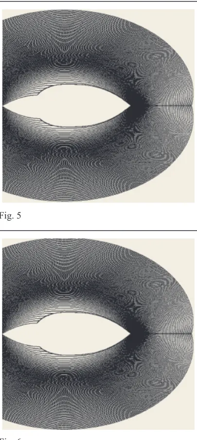
fl ow with Reynolds number R0 = 5000 and complex angles
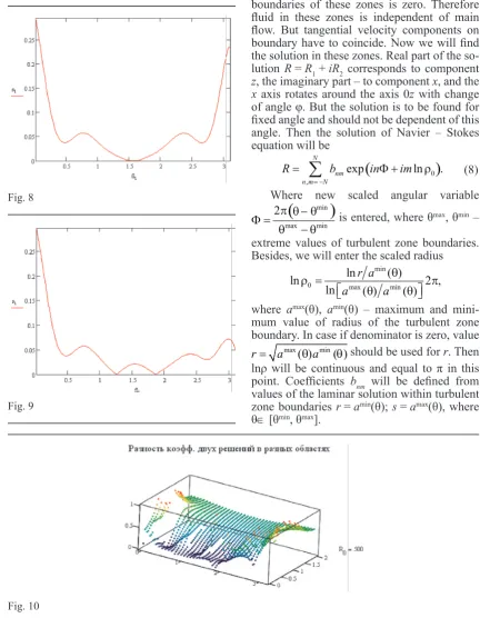
Two singular domains are seen in front of the sphere and behind the sphere. In these are-as, velocity corresponds to tangent line. Plot in Fig. 6 was calculated for the same parameters as plot in Fig. 5 but Reynolds number of the body is equal to R0 = 50000. The fl ow param-eters are maximal, pattern remains the same as for parameter R0 = 5000.
Fig. 7 was plotted for parameters
Rl(θl) = 0,1; R0 = 500.
Fig. 7
Velocity distribution is so that there is a singular domain in front of the sphere – in-compressible fl uid can not penetrate into this area. And this area, inaccessible for fl uid fl ow,
has large length that provides conditions for origin of long vortex path.
To change pattern, it is necessary to change angular boundaries and relation between
coef-fi cients Rl(θl). Besides, at large Reynolds num-ber, imaginary part increases and, hence rough-ness effect is rather large.
For incompressible liquid the equation of continuity along a current tube with longitudi-nal coordinate s has an equation . As the normal derivative from a normal com-ponent of speed is equal to zero for border of a special zone, we have constant longitudinal speed on border of a special zone. The con-vective term on border of a special zone is equal to zero. At that critical Reynolds num-ber for external region off the body is equal to , where a – specifi c body
size, lcr – length of the smooth body envelope when condition of complex coeffi cients Rl(θl) beginning is satisfi ed. Ratio is found from
non-linear equation for lcrfi nding, which cor-responds to beginning of complex solution.
For the plots computing, following equa-tion system was resolved in dimensionless co-ordinate system
x0 = –2; y0 [–4, 4].
Let us draw the curves for real boundaries of the area defi nition.
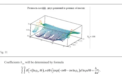
Vertical axis characterizes module of differ-ence between coeffi cients calculated for two dif-ferent areas. On horizontal axis the real angle θ0 is shown. In Fig. 8, the only root for small Reyn-olds number is shown. In Fig. 9, there are two real roots corresponding to the laminar mode with Reynolds number equal to R0 = 100.
Fig. 8
Fig. 9
In Fig. 10, 11 complex roots existence is shown, the roots are equal to
The imaginary axis values change in inter-val [0, 2], real axis inter-values – in interinter-val [0, π].
Description of Singular Domain
At that, solution for fl uid fl ow has dis-continuous zones, velocity perpendicular to boundaries of these zones is zero. Therefore
fl uid in these zones is independent of main
fl ow. But tangential velocity components on boundary have to coincide. Now we will fi nd the solution in these zones. Real part of the so-lution R = R1 + iR2 corresponds to component z, the imaginary part – to component x, and the x axis rotates around the axis 0z with change of angle φ. But the solution is to be found for
fi xed angle and should not be dependent of this angle. Then the solution of Navier – Stokes equation will be
(8)
Where new scaled angular variable
is entered, where θmax, θmin –
extreme values of turbulent zone boundaries. Besides, we will enter the scaled radius
where amax(θ), amin(θ) – maximum and
mini-mum value of radius of the turbulent zone boundary. In case if denominator is zero, value
should be used for r. Then lnρ will be continuous and equal to π in this point. Coeffi cients bnm will be defi ned from values of the laminar solution within turbulent zone boundaries r = amin(θ); s = amax(θ), where
θ [θmin, θmax].
Fig. 11
Coeffi cients bnm will be determined by formula
As boundary values at the beginning and the end of the period differ and area boundaries expressed in coordinates r, θ are not rectangular (in coordinates Φ, lnρ velocity on the boundary is variable), a series will be discontinuous, that is, the coeffi cient bnm decreases as when n, m → ∞, i.e. this solution is discrete. In singular domain, in coordinates lnρ, Φ, the solution is discrete due to discretization of functions R(lnρ0, Φ) in the form of discrete series. But as the description of singular domain is performed relative to coordinates lnρ0, Φ, the singular domain is discrete. Vortex path or pulsing turbulent mode with variable boundary is formed in this area at laminar mode.
The formula (8) can be rewritten in the form
(9)
where in this case we have
and then step with amplitude Anm and phase will be found from equations
where indexes n, m = –N, ..., –1, 1, ..., N.
It should be noted that A00 = b00. If the series in the left part of (9) is not summarized directly as this requires too large number of terms, then the right part of (9) will determine its discrete sum for fi nite number of terms. It should be noted that
Why the turbulent solution in singular do-main has the pulsing character with variable boundaries? The turbulent area boundary is not smooth function due to discreteness of the turbulent solution, unlike the laminar solution. This results in non-equality of tangential com-ponent of the solution and boundary pulsation in case of turbulent mode.
For description of laminar fl ow, it is nec-essary to enter dependence of specifi ed ra-dius on time
where Sh is a Strouchal number. At that, the pattern will fl uctuate with Strouchal frequency according to value of ln ρ0 and this will lead to vortexes rotation in opposite directions as the frequencies under condition
have different signs. At the same time, on the area boundary, frequency is zero, i.e. the solu-tion on boundary is continuous in laminar mode.
Solution of the Flow Problem for Arbitrary Smooth Body in Spherical Coordinate System
Laminar solution of the fl ow problem for arbitrary body in spherical coordinate system we regard resolved in the form of fi nal formula. That is, value of Reynolds number and pres-sure for laminar mode is found:
We resolve each Navier – Stokes equation
by multiplying by , integration over
inverse radius and angle θ, over two areas, which have one of the boundaries θl, l = 1, 2. We defi ned this boundary from equation
. As the equation for these angles fi nding is the second degree one, two angles, θk1, θk2, are found. We defi ne value θ0r(φ) for laminar solution and consider this in formula for Reynolds number taking area boundaries into account.
We do the same operation with other components of Reynolds numbers. Further we find out the solution by entering four un-known constants
it is possible to fi nd the problem solution for sphere, determining not laminar pressure, but such solution will be complicated. It is possible to add angle dependence of the sphere solution versus angle φ in Cartesian coordinate system and to solve a problem defi ning θ1(φ), θ2(φ), then dependence of the solution on angle φ will be found. At the same time, it is necessary to
keep dependence on spherical coordinate sys-tem at Cartesian components versus velocity and pressure. In curvilinear coordinate system, the derivative is determined by formula
Where
From this we defi ne through
depend-ence . The second derivatives with
respect to xl can be found similarly but in this case dependence on mixed derivatives with re-spect to r, θ, φ will occur.
At that, as velocity component
Rφ will occur. As θxl = θ0x, θyl = θ0y, θzl = θ0z, this dependence vanishes at small Reynolds number.
References
1. Monin A.S., Yaglom A.M. Statistical hydromechanics. Mechanic of turbulence. Part 1. – M.: Nauka, 1965. – Р. 640.
2. Shlikhting G. Theory of boundary layer. – M.: Nauka, 1974. – Р. 713.
3. Yakubovskiy E.G. Complex finite solutions of pri-vate derivative equations. Proceedings of International Scientific and Practical Conference. Theoretical and practi-cal aspects of natural and mathematipracti-cal sciences. – Novo-sibirsk: publisher “Sibak”, 2012, – Р. 19–30. – www.sibac. info http://sibac.info/index.php/2009-07-01-10-21-16/5809-2013-01-17-07-57-12.
4. Yakubovskiy E.G. Model of complex space. Proceed-ings of XIII International Scientifi c and Practical Conference. Vol. 1. – M.: “Institute of strategic researches”, publisher “Spet-skniga”, 2014. – Р. 26–32.
5. Yakubovskiy E.G. Model of complex space and images identifi cation. On a joint of sciences. Physical and chemical se-ries. Vol. 2. – Kazan, 2014. – Р. 186–187. – http://istina.msu.ru/ media/publications/article/211/bd0/6068343/raspoznavobrazov-withouteqution.pdf.
6. Yakubovskiy E.G. Determination of coeffi cient of re-sistance round pipe. the development of science in the 21st century: natural and technical sciences. – 2015. – 10 p. DOI: 10.17809/06(2015)-14.
7. Kittel Ch. Introduction to solid state physics. – M.: Nau-ka, 1978. – Р. 789.