University of Pennsylvania University of Pennsylvania
ScholarlyCommons
ScholarlyCommons
Publicly Accessible Penn Dissertations
2019
Range-Only Node Localization: The Arbitrary Anchor Case In
Range-Only Node Localization: The Arbitrary Anchor Case In
D-Dimensions
Dimensions
Pedro Paulo Ventura Tecchio University of Pennsylvania
Follow this and additional works at: https://repository.upenn.edu/edissertations Part of the Electrical and Electronics Commons
Recommended Citation Recommended Citation
Ventura Tecchio, Pedro Paulo, "Range-Only Node Localization: The Arbitrary Anchor Case In D-Dimensions" (2019). Publicly Accessible Penn Dissertations. 3519.
Range-Only Node Localization: The Arbitrary Anchor Case In D-Dimensions
Range-Only Node Localization: The Arbitrary Anchor Case In D-Dimensions
Abstract Abstract
This work is situated at the intersection of two large fields of research the Localization problem and applications in Wireless Networks. We are interested in providing good estimations for network node locations in a defined space based on sensor measurements. Many methods have being created for the localization problem, in special we have the classical Triangulation and Trilateration procedures and MultiDimensional Scaling. A more recent method, DILOC, utilizes barycentric coordinates in order to simplify part of the non-linearities inherent to this problem. Except for Triangulation in which we require angle measurements between nodes, the other cited methodologies require, typically only, range
measurements. Off course, there exists variants which allow the use of range and angle measurements. We specialize our interest in range only methods utilizing barycentric coordinates by first providing a novel way to compute barycentric coordinates for any possible node-neighbor spatial configuration in any given dimension. Which, we use as basis for our experiments with averaging processes and the
development of our centralized and distributed gradient descent algorithms. Our distributed algorithm is able to receive range measurements with noise of uncharacterized distributions as it inputs. Using simulations in Matlab, we provide comparisons of our algorithms with Matlab's MDS function. Lastly, we show our efforts on providing a physical network implementation utilizing existing small form factor computers, wireless communication modules and range sensors.
Degree Type Degree Type Dissertation
Degree Name Degree Name
Doctor of Philosophy (PhD)
Graduate Group Graduate Group
Electrical & Systems Engineering
First Advisor First Advisor George J. Pappas
Keywords Keywords
Barycentric coordinates, Cayley-Menger determinants, Localization, Wireless Sensor Networks
RANGE-ONLY NODE LOCALIZATION: THE ARBITRARY ANCHOR CASE IN D-DIMENSIONS
Pedro Paulo Ventura Tecchio
A DISSERTATION
in
Electrical and Systems Engineering
Presented to the Faculties of the University of Pennsylvania
in
Partial Fulfillment of the Requirements for the
Degree of Doctor of Philosophy
2019
Supervisor of Dissertation
George J. Pappas, Joseph Moore Professor and Chair
Graduate Group Chairperson
Victor M. Preciado, Associate Professor and Graduate Chair
Dissertation Committee
Victor M. Preciado, Associate Professor and Graduate Chair
RANGE-ONLY NODE LOCALIZATION: THE ARBITRARY ANCHOR CASE IN
D-DIMENSIONS
c
COPYRIGHT
2019
Pedro Paulo Ventura Tecchio
This work is licensed under the
Creative Commons Attribution
NonCommercial-ShareAlike 3.0
License
To view a copy of this license, visit
ACKNOWLEDGEMENT
I would like to thank my professors at University of Pennsylvania who guided and taught
me all the fundamental knowledge I acquired throughout these last six years. In special, I
would like to thank my advisor Professor George J. Pappas, for his help, guidance and
pa-tience. He provided me an environment were I could grow as a professional and individual.
Moreover, he was a constant among many variables.
I also offer my gratitude to Professor Jean Gallier,for his guidance while I was a student in
his class and later on during my Teaching Practicum. And to Professor Victor M. Preciado,
from whom I first learned about networks in general and who accepted to be chair of my
defense committee.
I thank Nikolay Atanasov and Shahin Shahrampour who I first met as fellow colleagues
in the Ph.D. program and with whom I started and continued the work presented in this
dissertation. I should also thank them for accepting my invitation to be part of my defense
committee as, now, Assistant Professors at University of California San Diego and Texas
A&M University respectively.
I also extend my thanks to my therapist Steven Adelman and my psychiatrist Deborah
Bernstein. They gave me emotional and medical support during my darkest moments as
a normal Ph.D. student.
My deepest acknowledgement and gratitude to my parents Cergio Tecchio and Vera Lucia
Ventura who provided me with anything and everything they could during these years.
Lastly, I thank the CAPES / Science Without Borders scholarship program from the
ABSTRACT
RANGE-ONLY NODE LOCALIZATION: THE ARBITRARY ANCHOR CASE IN
D-DIMENSIONS
Pedro Paulo Ventura Tecchio
George J. Pappas
This work is situated at the intersection of two large fields of research the Localization
problem and applications in Wireless Networks. We are interested in providing good
es-timations for network node locations in a defined space based on sensor measurements.
Many methods have being created for the localization problem, in special we have the
classical Triangulation and Trilateration procedures and MultiDimensional Scaling. A more
recent method, DILOC, utilizes barycentric coordinates in order to simplify part of the
non-linearities inherent to this problem. Except for Triangulation in which we require angle
measurements between nodes, the other cited methodologies require, typically only, range
measurements. Off course, there exists variants which allow the use of range and angle
measurements. We specialize our interest in range only methods utilizing barycentric
co-ordinates by first providing a novel way to compute barycentric coco-ordinates for any possible
node-neighbor spatial configuration in any given dimension. Which, we use as basis for
our experiments with averaging processes and the development of our centralized and
distributed gradient descent algorithms. Our distributed algorithm is able to receive range
measurements with noise of uncharacterized distributions as it inputs. Using simulations
in Matlab, we provide comparisons of our algorithms with Matlab’s MDS function. Lastly,
we show our efforts on providing a physical network implementation utilizing existing small
TABLE OF CONTENTS
ACKNOWLEDGEMENT . . . iv
ABSTRACT . . . v
LIST OF TABLES . . . viii
LIST OF ILLUSTRATIONS . . . xii
CHAPTER 1 : INTRODUCTION . . . 1
1.1 Related work . . . 9
CHAPTER 2 : PROBLEM DEFINITION . . . 14
CHAPTER 3 : A NOISELESS CENTRALIZED SOLUTION . . . 17
3.1 Fundamental theory . . . 18
3.2 Existing methods . . . 20
3.3 Our approach . . . 23
3.4 Algorithm complexity . . . 34
CHAPTER 4 : A NOISY DISTRIBUTED SOLUTION . . . 35
4.1 Averaging processes . . . 36
4.2 Centralized gradient descent . . . 37
4.3 Distributed Online Gradient Descent . . . 39
4.4 Algorithm complexity . . . 40
CHAPTER 5 : SIMULATIONS . . . 42
5.1 Noiseless centralized algorithms . . . 43
5.2 Noisy distributed algorithm . . . 52
CHAPTER 6 : EXPERIMENTS . . . 58
6.1 Base board options and operational system . . . 59
6.2 Range sensors . . . 61
CHAPTER 7 : CONCLUSION . . . 67
7.1 Future work directions . . . 68
APPENDIX . . . 70
LIST OF TABLES
LIST OF ILLUSTRATIONS
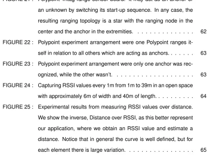
FIGURE 1 : Fig. 1a shows the general areas in which home automation is
sought using wireless node networks such as security, devices,
temperature, illumination and cloud services control. Meanwhile,
Fig. 1b shows devices already in large scale production which
seek to provide home automation features at least in determined
areas, for example we mention Google Nest and Amazon.com Echo. 2
FIGURE 2 : The future communication infrastructure based on 5G devices will
allow for heterogeneous devices to intercommunicate, Fig. 2a,
while a conceptual example of a self driven car is shown in Fig. 2b. 3
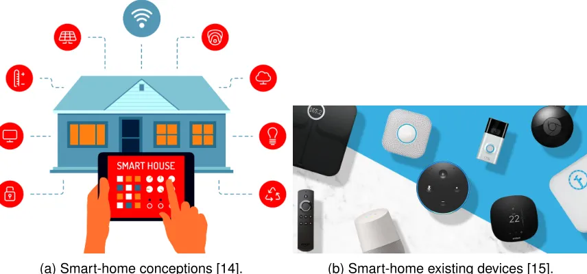
FIGURE 3 : Examples of wireless networked mobile robots used for
explo-ration Fig. 3a and for security Fig. 3b. . . 4
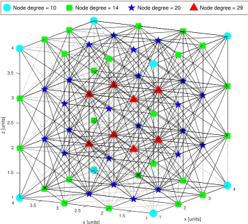
FIGURE 4 : Wireless node network example. Nodes are arranged in a
cu-bic lattice with lattice constant of 1 unit. We chose an inter-node
measuring and communication range of 2 units for all nodes. The
different vertex colors indicate nodes with different node degrees
as specified in its legends. . . 15
FIGURE 5 : Regions of different Barycentric Coordinate signs with non-zero
elements. Here, we consider only regions were coordinates are
either strictly positive or strictly negative. The black line segments
define the boundaries of the chosen points convex-hull. . . 27
FIGURE 6 : Regions of different Barycentric Coordinate signs with zero
ele-ments. In this figure, we specify some, but not all, possible regions
in space diving them by strictly positive, strictly negative or strictly
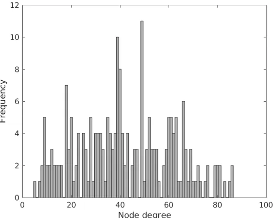
FIGURE 7 : GBC algorithm’s network example: node degree histogram. . . . 44
FIGURE 8 : Location estimates comparison: GBC, DILOC and Matlab’s MDS.
Black empty circles, squares and star are ground truth locations
for each node. Black lines define the convex-hull of anchors. Red
filled circles and stars are location estimates. Circles used for
lo-calized nodes; stars for unlolo-calized nodes. . . 45
FIGURE 9 : Some characteristics of Matlab’s MDS algorithm. . . 46
FIGURE 10 : Centralized GBM algorithm’s network examples: network graphs.
Anchor locations and convex-hull marked by black filled circles and
black continuous lines. Black empty circles mark ground truth
lo-cations. Dashed lines represent network range sensing and
com-munication connections. . . 48
FIGURE 11 : Centralized GBM algorithm’s solution estimates. Anchor locations
and convex-hull marked by black filled circles and black continuous
lines. Colored empty and filled circles mark ground truth locations
and location estimates; where each node has its own distinct color. 49
FIGURE 12 : Matlab MDS’s solution estimates. Anchor locations and
convex-hull marked by black filled circles and black continuous lines.
Col-ored empty and filled circles mark ground truth locations and
loca-tion estimates; where each node has its own distinct color. . . 49
FIGURE 13 : Matlab’s MDS stress value histogram for 100 simulations with one
replication each. . . 50
FIGURE 14 : Smallest and largest covariance matrices error ellipsoids for
Mat-lab’s MDS’s estimates. . . 50
FIGURE 15 : Non-zero elements of matrix W, communication weight matrix. Blue
dots are elements which it has in common with the respective
Pn l=1L(l)
T
L(l)matrix, while red asterisks are distinct. . . 51
FIGURE 17 : Distributed GBM algorithm’s solution trajectories over iterations.
Colored empty circles mark ground truth locations for each node.
Colored lines represent node estimates over iterations. Each node
is represented by a different color. . . 54
FIGURE 18 : Randomly generated sensor network with 10 unknown nodes and
4 anchors and trajectories of the node coordinate estimates over
time. Each color represents a different unknown node. The dotted,
dot dashed and full lines beginning with{2,D,4}and ending with
{,×,A}show the estimates over time obtained by the two-phase averaging Sec. 4.1 in equation (4.3), centralized gradient descent
Sec. 4.2 in equation (4.5) and distributed online gradient descent
Sec. 4.3 algorithms, respectively. The ground truth node locations
are marked by circles, while the black tetrahedron shows the
con-vex hull of the anchor nodes. As each node in the distributed
al-gorithm computes its own unknown node location estimates, it is
not possible to show the trajectories of the estimates of all nodes.
Instead, we show the trajectories of the estimated node locations
computed by one randomly chosen node. . . 56
FIGURE 19 : Root Mean Square Error (RMSE) of the node coordinate estimates
over time for the two-phase averaging Sec. 4.1 in equation (4.3),
the centralized gradient descent with Barzilai-Borwein and fixed
step sizes Sec. 4.2 in equation (4.5) and distributed online
gra-dient descent with proportional and constant variances Sec. 4.3
algorithms. As each node in the distributed algorithm computes
its own unknown node location estimates, we present RMSE
val-ues for the estimates of each node on the same plot. . . 57
FIGURE 20 : Beagle Bone Green Wireless compute board. It sports a mesh
FIGURE 21 : Polypoint Tritag range sensor board. It may act as an anchor or
an unknown by switching its start-up sequence. In any case, the
resulting ranging topology is a star with the ranging node in the
center and the anchor in the extremities. . . 62
FIGURE 22 : Polypoint experiment arrangement were one Polypoint ranges
it-self in relation to all others which are acting as anchors. . . 63
FIGURE 23 : Polypoint experiment arrangement were only one anchor was
rec-ognized, while the other wasn’t. . . 63
FIGURE 24 : Capturing RSSI values every 1m from 1m to 39m in an open space
with approximately 6m of width and 40m of length. . . 64
FIGURE 25 : Experimental results from measuring RSSI values over distance.
We show the inverse, Distance over RSSI, as this better represent
our application, where we obtain an RSSI value and estimate a
distance. Notice that in general the curve is well defined, but for
CHAPTER 1 : INTRODUCTION
There exists great public interest in large heterogeneous wireless networks. By
heteroge-neous wireless networks, we mean a wireless network of diverse distinct devices, which
may run any kind of software over different hardware platforms. The most common topics
involving these networks are IoT - Internet of Things [1, 2], VANETs - Vehicular ad-hoc
net-works [3, 4], home automation netnet-works [5–7], mobile robots and robotic sensors [8–10].
One simple example of an IoT is a modern technological driven home, where multiple
dif-ferent appliances and electrical equipment of distinct brands communicate among
them-selves and/or with user interfaces, usually built as apps in mobile smart-phones, to provide
greater comfort and capabilities for homeowners [5–7]. An early implementation of such
technology is the popular Nest thermostat witch was first created as a home temperature
control center with the ability to learn and to integrate via WiFi to other devices. Later, other
products from the same company were marketed such as smoke andCO2 detector and a
complement of interconnected cameras. Nowadays, the brand and technology is owned
by the Google group under their holding company Alphabet Inc and these devices are
mar-keted to work in an environment of up to 3000 different products including Google’s own
voice interface ”Hello Google” which enables them to use voice control. Another leader in
this segment is Amazon.com Inc. which similarly works in partnership with other
compa-nies to enable its own ”Alexa” voice interface to control different devices around the same
WiFi or Bluetooth networks.
Also in the segment of home automation, we can attach personal health care devices and
products for personal everyday use such as electric toothbrushes and Bipap machines
which interconnect with smartphones in order to provide historical data and a user friendly
control interface. In a more extreme case, we can include future deployment of mobile
au-tonomous robots for the health care of its residents [11–13]. We believe that such robots
re-(a) Smart-home conceptions [14]. (b) Smart-home existing devices [15].
Figure 1: Fig. 1a shows the general areas in which home automation is sought using wire-less node networks such as security, devices, temperature, illumination and cloud services control. Meanwhile, Fig. 1b shows devices already in large scale production which seek to provide home automation features at least in determined areas, for example we mention Google Nest and Amazon.com Echo.
quired, specially for tasks which are considered a chore by their families or in which the
family members are not trained to perform or are not able to, as examples we cite cleaning
of human waste, application of intravenous medicines or physically lifting impaired people.
Meanwhile, vehicle-to-vehicle and vehicle-to-roadside communication architectures are the
fundamental blocks of VANETs. These communication protocols are being built in order
to enable new vehicle features and road services, such as vehicle security through shared
information about threats, traffic management and better performance and reliability of
self-driven cars [3, 4, 16–20]. Up to the publication of this dissertation, there is no common
communication and sensing network protocols and standards, as such technologies are
being extensively researched and implemented by numerous vehicles manufactures,
tech-nological companies and academy. The autonomous car may not be the hot topic of the
moment in the academic world, but it is still in the process of being studied and readied
(a) 5G enabled communication infrastructure [21]. (b) Self driven car [22].
Figure 2: The future communication infrastructure based on 5G devices will allow for het-erogeneous devices to intercommunicate, Fig. 2a, while a conceptual example of a self driven car is shown in Fig. 2b.
will be able to self coordinate and also plan their operation in a cooperative way with other
cars and with the road infrastructure enabling for example local and global traffic
manage-ment and control; road alerts propagated throughout the network so that cars can plan
their actions in advance, and vehicle platooning in small (road-wide) to large (city-wide)
formations. Moreover, in the near future, maybe a few decades or so, vehicle accidents
with injured or dead passengers or pedestrians will be seldom seen, as there will exist less
and less human interference in the system with increasing redundancy of sensors, network
communication and system intelligence.
Even if one may not consider future vehicles as mobile robots and we may also disregard
home automation robots, one may not forget about the large insurgency of drones that is
happening now. Major and minor companies are studying ways to apply drone technology
to either its operations or products. A famous example is again Amazon.com Inc. which
seeks to utilize drones as a mean of package delivery in highly populated cities. Another
major segment in which drones are being researched for and applied are law
enforce-ment, rescue and military. In these, drones may be used for exploration, infiltration, target
search and track, target pacification, packages, objects and ordnance delivery among
oth-ers. Meanwhile, their utilization has been a topic of concern among some legislators and
(a) Mobile robots used in undersea explo-ration [23].
(b) Mobile robost used for site security [24].
Figure 3: Examples of wireless networked mobile robots used for exploration Fig. 3a and for security Fig. 3b.
other recording devices; cause accidents and property damage and also be used for
ne-farious and unlawful activities.
While many devices and applications are already being marketed and used in somewhat
niche markets, most of them are still being researched and developed. Among the different
lines of research and development, our interest lies in the exploration of a topic that they
usually have in common, the need to known where they are being used. This need may be
a focus of interest among device users and maintainers or among the devices themselves.
The ability of localize oneself in the environment is an important feature to many systems,
as it may influence its behavior and functionality. A human placed in an unknown
envi-ronment will have difficulties to live in it effectively, the same can be said to a sensor or
robot, as they will possibly not be able to effectively perform their tasks. Besides the
ear-lier examples, we can mention a simple one: a network of atmospheric sensors used to
obtain climate data for general use. If one does not known the position of these sensors,
their gathered information becomes almost meaningless. It is a major problem to know a
hurricane is coming but not knowing where it is and to where it is going. One may mention
that in such an example, all sensors will be placed in fixed and GPS enabled locations, so
case does not happen, for example inside a building or with moving nodes?
As can be inferred, our interest lies in localizing nodes of a network, more specifically static
ones which are able to range themselves in relation to their neighbors. We focus on static
networks as they provide an entry point for the localization problem and are also largely
used in homes, business and industrial applications. On another hand, we were able to
supplement the existing theory of static network localization in a meaningful way, by
pro-viding a formulation that works in any possible spatial dimension and with fewer constraints
on the network. Regarding the utilization of range measurements alone, one point of view
it that having both range and bearing measurements among nodes may provide a larger
amount of information, another is that the restriction to range only measurements should
be seen as a feature as we only require partial information about inter node positioning
and therefore less sensors. Having said so, we do not mean to imply we are not
inter-ested in studying the possibility of integrating bearing measurements to our methodology
in the near future, as it is possible that having both will enable us to create a more efficient
method.
For now, our proposed method is able to localize nodes in a static network provided that
we give the actual and noiseless location ofd+ 1 nodes of the network ind-dimensional Euclidean space (which are called anchor nodes), the range measurements between all
neighboring nodes and that each node must have at leastd+ 1neighbors. It may be the case, that some nodes satisfy these constraints, but are not localizable, which will happen
if their neighbors are not localizable themselves. So an unlocalizable node may affect an
entire segment of a network. Therefore, localizable nodes form a network with anchor
nodes, in which, nodes have at least d+ 1 neighbors. In spite of those requirements, there is no restriction on the position of nodes in relation to anchors as exists among
other methods which we will specify in the next section. This is an important feature, as
it enables the utilization of our algorithm to localize more diverse networks regardless of
where other methods would require two sets of4anchors, in which case at most3may be
used in both sets, and two runs of the algorithm to localize nodes in a rectangular prism
shaped environment (a common room rectangular floored room), ours would only require
the application of the algorithm once with4anchors.
We formalize our localization problem in Chapter 2, then we explain our theoretical
reason-ing in Chapters 3 and 4. In these chapters, we develop our method based on Barycentric
Coordinates, which may be easily understood as computing proportional volumes of
re-gion segments in space defined by the location of their vertices. In other words, given a
d-dimensional space, one region in it is defined usingd+ 1points as vertices of this region, which actually is a simplex. Then by choosing a different point in the same space and
computing the volume of each possible simplices formed by substituting one point of the
previous set with this new point, we can compare the volumes of the new regions with the
old one by division, which is exactly how barycentric coordinates are calculated. Therefore,
in the case of a network, each node is treated as a point in space with a Cartesian
coordi-nate, then we choosed+ 1neighbors of this node which form a simplex and compute the barycentric coordinates for each node in relation to each chosen subset of its neighbors.
These coordinates form a linear system of equations where the node Cartesian
coordi-nates are the unknown variables. Therefore, by isolating the anchor coordicoordi-nates which are
known from the rest of unknown variables, one may solve this linear system and compute
all unknown node coordinates.
One may ask, how do we compute the simplices volumes if we are only measuring
inter-node ranges? If one consult the existing literature, one will probably find the concept
of Cayley-Menger determinant. This determinant relates the Eucldiean Distance Matrix,
matrix formed by squared Euclidean distances between each pair of points in a given
set ofd+ 1elements in d-dimensional Euclidean space, with the simplex volume formed by such points squared. As the Euclidean distance is the same as the range between
coordinates. But there is a catch is this relation. As mentioned, the value obtained from
computing Cayley-Menger determinant is proportional to the square value of the simplex
volume, so one does not know which sign, positive or negative, to use in order to compute
barycentric coordinates.
If one restrict its nodes to always be inside the convex hull of their neighbors, and by
extension, the entire network should be inside the convex hull of the anchors, one is able
to ignore this sign problem, as the correct sign should always be positive in this case by
construction. This fact is explored by the vast majority of network localization works that
exist nowadays. Other works are either restricted in the space dimension or use mixed
approaches to solve the localization problem. We on the other hand, developed a method
to compute barycentric coordinates with their correct signs by applying a more general
form of the previous determinant called Cayley-Menger bi-determinant, which is not so
commonly found in the related literature. This bi-determinant takes to distinct sets of points
and compute a value proportional to the multiplication of their simplices volumes, which we
can use to compute barycentric coordinates and proceed as previously explained in other
to compute the unknown node coordinates.
So far, we talked about computing the Cartesian coordinates without mentioning anything
about noise or how does our algorithm operates. It is because this theory enables us to
solve the problem in centralized form with noiseless range measurements, but what
hap-pens when that is not the case? Adding noise to our measurements becomes a mess,
even using simple zero mean additive Gaussian noise to each measurement makes the
output of the Cayley-Menger bi-determinant have an unknown probability distribution with
complex terms formed by sums of products and divisions of Chi-Squared random
vari-ables. So the standard approach to solve this problem in closed form becomes unfeasible.
Following, some related works we decided to apply an averaging process in all range
measurements individually, as we consider that they will have at most zero mean
distribution here. Then, by the Law of Large Numbers the average should converge to
an approximate noiseless range value when one approaches a sufficiently high number
of noisy measurements. Therefore, in theory in order to easily solve this problem, one
should acquire a large number of measurements, compute the Cayley-Menger
determi-nants, compute barycentric coordinates and solve the linear system of equations arriving
to a probably good enough location estimates for each unknown node. As always, in
prac-tice it does not always work. Numerical errors from all non linearly computation may lead
to high discrepancies in the actual computed values for the barycentric coordinates from
one set of measurements to another. The easiest solution was to average the barycentric
coordinates again in order to suppress such problems. As we did so, we arrive to our first
centralized method able to provide somewhat good estimates over time.
In order to arrive to a distributed solution, we first experimented with a centralized gradient
descent algorithm that worked as intended with both fixed and dynamic step sizes. Then,
we modified our mathematical formulation to apply an existing theoretical algorithm to solve
optimization problems in distributed systems over a given time horizon. This choice proved
fruitful as we were able to finally solve our localization problem with noisy range
measure-ments in a distributed form. Simulated experimeasure-ments where we applied our algorithms to
randomly generated networks will be shown in Chapter 5 with the respective discussions.
Lastly, during our theory development, we also sought to provide a physical platform in
or-der to demonstrate our work, but we were not completely successful in this front. As will be
discussed in Chapter 6, we provide in Appendix A.2.1 a recipe of sorts on how to compile,
configure and apply a Linux distribution with the correct drivers in order to use our chosen
platform and sensor suite with the necessary network configuration and data extraction
software. Our platform was constructed around a Beagle Bone Green Wireless board with
integrated WiFi module capable of operating in mesh networks. We notice that this was
the first board in the market able to do so, while nowadays there may be other possibilities
topology which disallowed us to use it in real time operations as one had to keep switching
it on and off to change its configuration from anchor to unknown node, i.e. in the entire
sensor network only one device ranged itself at a given time in relation to all others, so
it was required to reset it every time one wanted obtain range measurements from other
devices. Because of this constraint, we sought other sensors without much success. At
one point, we finally decided to use RSS - Received Signal Strength measurements from
the WiFi module as a means of estimating range measurements. We did some
experi-ments at first in open space without occlusions and the results were satisfactory, but later
on when working inside of a building with walls and other objects cluttering the space in
which the sensors were positioned, our first measurement model became irrelevant. Even
a change in the sensor height in relation to the ground would change the RSS
measure-ments received. Therefore, lacking an appropriate range sensor, we decided to focus on
the theoretical aspect of the problem.
In the next section we will introduce the relevant existing works and start introducing the
range only localization problem with arbitrary anchor placement in a more formal setting.
1.1. Related work
An heterogeneous wireless network must satisfy a series of constraints in order to work
correctly as intended by its stakeholders, be its developers, maintainers and users. One
main aspect of such networks is that it may contain both static and or mobile nodes which
are loaded with sensors necessary for their independent or communal operations. In either
case, it is most likely that their location will influence their operation andvice versa.
There-fore, it is important for each node in a network to know its current location over time with
respect to some local or global frame of reference. Relative localization is especially
chal-lenging but also most important to solve robustly in harsh operational conditions, where
GPS access is denied, the surroundings are featureless, and the sensed information is
lower-dimensional than the sensor states of interest (e.g.bearing-only or range-only
by significant measurement noise. To correctly determine a frame of reference, it is usually
required that locations of a small subset of its nodes, called anchor nodes, are known.
Throughout this paper we call all other nodes unknowns as they are not localized.
The localization problem of wireless networks has been considered in 2 and 3 dimensions,
with some working in higher generic dimensions, using different measurement types and
noise distributions. Range and bearing measurements are utilized in some methodologies
[25–27], while others rely only on one of them such as bearing-only [28–31] and
range-only measurements [32–38]. Typically most algorithms start in a centralized fashion [39–
42], i.e. all network information is sent to a ”central” node responsible for more intense
computational needs to localize all network nodes; else, if each node remains responsible
for its own localization based on shared local information, the algorithm is called distributed
[27, 30, 32–35, 38, 43–58].
Multiple different methodologies have been developed over years of research in
localiza-tion. One of the most fundamental methods is based on Triangulation [40–42] or more
commonly Trilateration [8, 59]. The later can be summarized as the iterative resolution
of a non-linear system of equations relating the range measurement between nodes and
the Euclidean distance between the location estimates for each unknown node. The 2-D
example below demonstrate the set of equations needed to localize node l in relation to nodesi, j, k:
||xl−xi||2 = zli ||xl−xj||2 = zlj ||xl−xk||2 = zlk
(1.1)
As mentioned, Trilateration methods work by localizing one unknown node at each iteration
based on existing anchor nodes or already localized unknown nodes, which is an iterative
process. Different from this, there are methodologies in which all necessary information is
gathered and the localization of all nodes is done simultaneously either in a centralized or
- MultiDimensional Scaling [35, 39, 63, 64] and barycentric coordinates based methods
[32–35, 48, 50–52, 54]. From these, we emphasize both MultiDimensional Scaling and
barycentric methods. We utilize MDS as a benchmark tool for our proposed algorithm
which is based on barycentric coordinates. The classical MDS approach is to solve an
optimization problem minimizing the following function:
Stress(x1,· · ·,xn) =
X
i,j
(Zij − ||xi−xj||2)2
X
i,j
Zij2
1/2
(1.2)
In spite of not having a convex nor linear function to be optimized, MDS methods have
an advantage: they can be solved through the manipulation of its algebraic equations in
matrix form, so that solving the minimization problem becomes equivalent to eigenvalue
and eigenvector decomposition of a matrix, for which exists optimized algorithms. Their
disadvantage is that their solution is dependent of initial estimates. Therefore, using
ran-dom initialization may incur on solutions with stress varying from small to large values, so
one needs to run the algorithm multiple times in order to get a good solution.
The barycentric coordinates approach seeks to hide all non-linearities of this problem in
the computation of barycentric coordinates. So, after one finds all barycentric coordinates
for all nodes in the network, the solution of the noiseless system becomes as easy as
solving a linear system. This method was first proposed by Khan et al. in [32]. It is
interesting to notice that the system becomes automatically distributed along the many
nodes of the network, i.e. each node is able to compute its barycentric coordinates with
local information.
This method becomes harder to solve whenever there is noise added to the range
mea-surements, as one need to pay attention to the errors inserted on the computation of the
heavily non-linear set of equations involved on the computation of all barycentric
for barycentric coordinates given even simple additive Gaussian noise to range
measure-ments. In order to solve this last problem, Khanet al. proposed an algorithm based on
averaging processes [34].
Multiple variations of the first barycentric algorithm [32] were proposed such as [33–35,
48–52, 54]. Khanet al. in special provide us with a diverse collection of works extending
this framework in static and mobile networks and in different applications where unknown
nodes are strictly inside the convex-hull of anchors [32–34,48,49,52]. In another direction,
Diaoet al. proposed in [33] an algorithm for the 2-D case, that allow an arbitrary
position-ing of anchors among unknown nodes. Unfortunately, their line of reasonposition-ing to solve the
localization problem was based on the geometrical identification of all conditions
neces-sary to correctly compute barycentric coordinate’s signs in more than 2-D. In [35], Hanet
al. proposed a hybrid approach of mixing barycentric coordinates with MDS to solve the
same problem in3-dimensions.
In this work, we leverage the definition of Cayley-Menger bi-determinants found in [8] to
deduce a new formulation of barycentric coordinates which allow us to extend the previous
results of Diao et al. to the generic d-dimensional space. As will be shown, we provide a distributed algorithm able to localize nodes in d-dimensional Euclidean space with only inter-node noisy measurements and a small subset of d+ 1 anchors. In our algorithm, there is no assumption about the position of any node in the network;i. e. anchors can be
anywhere in relation to unknowns. Moreover, we do not assume any previous knowledge
about noise characteristics of any range measurement. Locations of anchors which should
be noiseless are an exception, though.
Excluding [35], which utilizes a hybrid approach of using barycentric coordinates and MDS
- MultiDimensional Scaling; previous works known to use barycentric coordinates, either
restrict the dimension of the problem to two [33] or assume some specific arrangement for
anchor and unknown nodes [32, 34, 48, 49, 52]. While our approach may still present some
pure way to solve the localization problem of anyd-dimensional static node network using barycentric coordinates with range measurements andd+ 1node locations.
Even though, by our knowledge, no practical application for localization problems in greater
than 3-dimensional Euclidean spaces exists nowadays; we still believe it is necessary to
provide the related theory for such a case, as it may occur in the future.
Succinctly, our main contributions are:
• Provide a way to compute barycentric coordinates for any node arrangement in d -dimensional Euclidean space.
• Provide a centralized algorithm able to solve the localization problem ofd-dimensional static networks based on noiseless range measurements andd+ 1node locations.
• Provide a distributed algorithm able to solve the previous localization algorithm under
CHAPTER 2 : PROBLEM DEFINITION
A static sensor network in d-dimension Euclidean space can be modeled as a weighted directed graphG={V,E,Z}, with vertex setV :={1,2, . . . , n}. From this set, we define the subsetAof anchor nodes with known locations and the subset U of nodes with unknown
locations, such that V = AS
U and AT
U = ∅. We refer to the Cartesian coordinates
xi ∈ Rd of node i ∈ V as its location. Therefore, the set of all node locations is X, of anchor nodes isXAand of unknowns isXU.
An edge(i, j)∈ E, whereE ⊆ V × V, exists whenever nodesiandj are able to commu-nicate and measure their relative distances, d(xi,xj) = ||xi−xj||2. Supposing that each
node i ∈ V has a maximum sensing range ri ∈ R>0, an edge between node pair (i, j)
exists ifd(xi,xj)≤min{ri, rj}.
An example of such a network in 3-D is shown in Fig. 4. In this example, all 64 nodes
are arranged in a cubic lattice with a lattice constant of 1 unit. Inter-node measuring and
communication ranges are 2 units,ri = 2,1≤i≤m. Fig. 4 also shows the node degree1
of each vertex in this network example.
We suppose that each pair of nodes(i, j)∈ E obtains range measurements over timet= 1, . . . , T, which can be arranged in a set of square matrices such asZ :={Z1, Z2, . . . , ZT}
withZt∈Rn×n∀t. Moreover,[Zt]ij =d(xi,xj) +δij(t)whereδij(t), for all pairs(i, j)∈ E in
time, are independent identically distributed (iid) random variables with unknown probability
distribution. Assumingδij(t)andδji(t)are independent, the measured quantities[Zt]ij and
[Zt]ji are distinct random variables and thus the generated graph is directed. Conversely,
the noiseless case leads to an undirected graph formulation.
Therefore, based on the previous concepts, we can formulate the general form of the
localization problem as the following:
1
4
3 1
1.5
x [units] 2
4 2.5
z [units]
3
3.5 3.5
4
2 3
y [units]
2.5 2
1.5 1
1
Node degree = 10 Node degree = 14 Node degree = 20 Node degree = 29
Figure 4: Wireless node network example. Nodes are arranged in a cubic lattice with lattice constant of 1 unit. We chose an inter-node measuring and communication range of 2 units for all nodes. The different vertex colors indicate nodes with different node degrees as specified in its legends.
Problem. Given the anchor node locationsXA ⊂ X of a static sensor network and noisy
range measurementsZ, estimate the locations of all unknown nodesXU ⊂ X.
In the next section, we define Cayley-Menger bi-determinants and barycentric coordinates.
Then, we show how to use the first to compute the second for any possible node
arrange-ment. Next, based on barycentric coordinates, we show how to solve the centralized
noise-less case of the generic localization problem and later the distributed noisy case. But first,
let us summarize in Table 1 our most used symbols with their meaning for future reference.
Table 1: Symbol notation
Symbol Meaning
i, j, k Generic indices
l Index referencing thelth node
t Index referencing time iteration
d Number of dimensions
n Number of nodesn:=|V|
a Number of anchor nodesa:=|A|
u Number of unknown nodesu:=|U |
rl Maximum sense range of nodel
δij(t) Random noise at edge(i, j)at timet
Kn Group of complete graphs withnvertices
P,Q Generic sets
V Set of vertices or nodes
E Set of edges
Z Set of range measurement matrices
A Subset of anchor nodes
U Subset of unknown nodes
N(l) Set of neighbors of nodel
I(l) Family of sets ofd+ 1indexes given by all possible combinations of
d+ 1neighbors of nodelwhich form a subgraph inKd+1
X(l) Family of sets of Cartesian coordinates of neighbors oflgiven byI(l)
Xi(l) ithset of familyX(l)
b Xi(l)
j i
thset of familyX(l)withjthelement modified
p,q Generic real column vectors with some specified dimension 1 Vector of ones with correct dimension
xl,x(l) Location of nodelinRd
[xl]i,xi(l) Element atith-row of vectorx(l)
P, Q Generic matrices with some specified dimension
X Location matrix inRd×n
Zt Range measurement matrix at timet
Ll,L(l) Matrix of barycentric coordinates of nodel
[Ll]ij,L(ijl) Element atith-row andjth-column of matrixL(l)
L(l) Generalized barycentric matrix (GBC) of nodel
L(:lA) The columns of GBC oflthat are indexed byA
CHAPTER 3 : A NOISELESS CENTRALIZED SOLUTION
We start our endeavor to solve the localization problem proposed in Chapter 2 in a
cen-tralized form under noiseless range measurements by defining the theoretical background
on Cayley-Menger determinants, bi-determinants and barycentric coordinates. These
con-cepts will prove to be fundamental to our proposed centralized algorithm, as one can utilize
Cayley-Menger determinants and bi-determinants to compute barycentric coordinates and
with them one is able to solve the localization problem by simply computing the solution of
a linear system.
Cayley-Menger determinants were extensively used by Blumenthal in his book about
Dis-tance Geometry [65], were he defined and proved this determinants property of relating
Eu-clidean Distance Matrices proportionally to the square of the signed volume of the simplex
formed by the set ofd+ 1points utilized in the Euclidean Distance Matrix ind-dimensions. Then, we summarize how these concepts were applied under different assumptions by
Khan et al. in [32] and by Diaoet al. in [33], which we consider to be the precursors of
our solution. The former is the first work to utilize barycentric coordinates to solve
range-only localization in wireless networks, while the later is an extension or modification of the
former seeking to allow arbitrary placement of anchors among unknown nodes in the two
dimensional case. By arbitrary placement of anchor nodes, we mean that anchor and
un-known nodes may be placed randomly, but they must satisfy the criterion of having at least
d+ 1distinct neighbors that form a simplex of non-zero volume. This is an extension on Khan’s work which required all nodes to be place inside the convex-hull of a subset of their
neighbors and consequently, to have all unknown nodes inside the convex-hull of thed+ 1 anchor nodes.
In [8], we discovered the concept of Cayley-Menger bi-determinants without any formal
proof, which we later constructed based on Blumenthal’s proof of the determinant, and
determinant. This choice proved extremely successful, as it allowed us to develop a
com-putationally efficient way to calculate correctly signed barycentric coordinates for any set
ofd+ 1point ind-dimensional Euclidean space based on their Cartesian coordinates. The ability to compute all signs is fundamental to our work as it enables us to provide an
al-ternative solution for Diao’s work in the 2-D case, moreover it also allowed us to extend
their idea to any possible dimension. It is not as fundamental to works which follow Khan’s
assumption of having nodes inside the convex-hull of their neighbors, as in this case all
signs are strictly positive.
Later on we provide the best possible least squares estimate for our proposed localization
problem via the solution of a over-determined solution, moreover if the inverse of a
sub-matrix of this system exists, then we are able to compute the correct and full solution for
each unknown node Cartesian coordinate.
3.1. Fundamental theory
3.1.1. Cayley-Menger determinant
Cayley-Menger determinants, [32–34, 65], provide a relation between Euclidean distances
of points in space and the signed volume of the simplex formed by such points as seen
below in Definition 1 and Theorem 1.
Definition 1. Let the tuple of d+ 1points, P = (p0, . . . ,pd), be defined by its Cartesian
coordinates, such thatpi ∈Rdfor0≤i≤d. Then, the Cayley-Menger determinant ofP is
defined as follows:
D(P) =D(p0, . . . ,pd) =
2 −1 2 d+1
0 1 1 . . . 1
1 0 d(p0,p1)2 . . . d(p0,pd)2 1 d(p1,p0)2 0 . . . d(p1,pd)2
..
. ... ... . .. ...
Theorem 1. The Cayley-Menger determinant of a tuple ofd+1points inRd,P = (p0, . . . ,pd),
is related to the square of its signed volume as in
D(P) = (d!)2Vol(P)2. (3.2)
Proof. See Appendix A.1 by takingQ=P.
But, why is this Cayley-Menger determinant so important for our problem solution? One
may reply, that by actually changing the computed Euclidean distances of points in P to
actual range measurements[Zt]ij∀(i, j)∈ E, one may actually compute the experimental
signed volume squared, which will be used to compute barycentric coordinates in the next
section.
3.1.2. Applying barycentric coordinates
Barycentric coordinates are usually defined using concepts of points, affine spaces and
affine frames. An affine space P is defined by a collection of points, a vector space
and a function. An affine frame is a set of points in an affine space with origin p0,
{p0,p1,· · ·,pd}, such that vectors {−−−→p0p1,−−−→p0p2,· · · ,−−−→p0pd}are linearly independent, i.e.
they form a base for the embedded vector space−→P. By taking a field Ksuch as R, one
can define barycentric coordinates as follows:
Definition 2([66, Prop.3.6.2 Modified]). Let{pi}i=0,1,...,dbe a frame for an affine spaceP.
For any (point)p∈Pthere existλi ∈K,0≤i≤d, such thatPiλi = 1andp =Piλipi.
The scalarsλiare uniquely defined by this property and are called barycentric coordinates
ofpin the frame{pi}i=0,1,...,d.
From Definition 2, one can infer that in order to localize an unknown node in the network,
form an affine frame for the inherent affine space. Also, from Definition 2 and Theorem 1
one may compute theabsolute value of any barycentric coordinate from a tuple of points
in space as given next:
Definition 3. Let the tupleP = (p0,· · · ,pd)be a frame for an affine spaceP. Then, given
a pointp ∈ P, theabsolute value of its barycentric coordinates in relation to the tupleP
is:
|λi|= s
D(p0, . . . ,pi−1,p,pi+1, . . . ,pd)
D(p0, . . . ,pd)
(3.3)
Later, in Section 3.3.2 we will provide a formal and novel way to compute the true signed
barycentric coordinates for any point p ∈ Pin relation to the tupleP. So far, in order to
present the aforementioned summary of Khanet al.’s DILOC, [32], and Diaoet al.’s ECHO,
[33], the existing definitions will suffice.
3.2. Existing methods
3.2.1. DILOC
In [32], Khanet al.proposed the DILOC algorithm utilizing barycentric coordinates to solve
localization problems in wireless networks. We will summarize this algorithm through an
example in 2-D space. So, let points{pi,pj,pk,pl} ∈Pbe the locations of some nodes in
a network. Then, we can calculate the magnitude of barycentric coordinates of pointlas:
|λ(il)|=
qD(p
l,pj,pk)
D(pi,pj,pk) |λ
(l)
j |= q
D(pi,pl,pk)
D(pi,pj,pk) |λ
(l)
k |= qD(p
i,pj,pl)
D(pi,pj,pk) (3.4)
Now, by definition of barycentric networks in Definition 2, their sum must be equal to one.
Therefore, if we suppose that nodelis inside the convex-hull of the other nodes, then the sum of its barycentric coordinates magnitudes should also sum to one. This acts as a
inclusion test to verify if nodes are inside or outside the convex-hull of its neighbors.
a pointp∈P,pis inside the convex-hull ofP if and only if
n X
i=1
|λ(il)|= 1. (3.5)
Where,|λ(il)|= 0ifi /∈ P. We call this the inclusion test.
Therefore, if a node passes the inclusion test for a subset of its neighbors, it can be
cor-rectly localize according to the following set of equations which define DILOC:
p(l,t+1)=Pn i=1λ
(l)
i p(i,t) iflis unknown,
p(l,t+1)=p(l,t) iflis anchor.
(3.6)
The main advantage of DILOC’s algorithm is that it can be written as an Absorbing Markov
process, which allows one to use its theory to prove the method’s convergence and
facili-tates its usability in many other setups such as [48, 49]. Next, we define ECHO which was
proposed by Diaoet al. in [33] as an extension of DILOC.
3.2.2. ECHO
This algorithm differentiates itself from DILOC in two major ways. First, it proposes a way to
compute the correct barycentric coordinate signs in the two dimensional case. This allows
one to utilize any possible subset of neighbors of a node to compute its barycentric
coor-dinates. Second, it defines the generalized barycentric coordinates which are then used
to form a linear system able to solve the localization problem under some assumptions.
Diaoet al. in [33], proposes Algorithm 1 to compute the correct signs for barycentric
coor-dinates in the two dimensional case. The algorithm is composed of a series of if and else
statements, which dissects all possible node arrangements. Moreover, all of these checks
must be done for each possible neighboring node combination of d+ 1 nodes for each node in the network. This is done in order to compute, what they called the Generalized
Barycentric Coordinates, which we present in Definition 5.
Algorithm 1Signs of barycentric coordinates in 2D.
Input: |λ(il)|,|λ(jl)|,|λ(kl)|, Zli, Zlj, Zlk, Zij, Zik, Zjk
Output: σ(il), σj(l), σ(kl)
if σ(il)|λi(l)|+σj(l)|λj(l)|+σk(l)|λ(kl)|= 1has unique solutionthen
return (σ(il), σj(l), σk(l))
else if|λ(il)|== 0or|λj(l)|== 0or|λ(kl)|== 0then
if|λ(jl)| ≤1and|λ(kl)| ≤1then
return (σi(l), σj(l), σ(kl)) = (1,1,1)
else if|λ(jl)|>1and|λj(l)|>|λ(kl)|then
return (σi(l), σj(l), σ(kl)) = (1,1,−1)
else if|λ(kl)|>1and|λk(l)|>|λ(ll)|then
return (σi(l), σj(l), σ(kl)) = (1,−1,1)
end if
else ifZlj ==ZikandZlk ==ZijandZli2 == 2Zij2 + 2Zik2 −Zjk2 then
return (σ(il), σ(jl), σk(l)) = (−1,1,1)
else ifZlj < Zij2 +Zli2 then
return (σ(il), σj(l), σk(l)) = (1,1,−1)
else ifZlj > Zij2 +Zli2 then
return (σ(il), σj(l), σk(l)) = (1,−1,1)
end if
barycentric coordinate,λl∈Rm, can be computed as follows
λTl = 1
|I(l)|
|I(l)|
X
i=1
L(ijl), (3.7)
whereL(l) is the matrix formed by concatenating all possible barycentric coordinates λT
which are computed using both Definition 3 and Algorithm 1.
As the generalized barycentric coordinates in equation (3.7) are computed through
aver-aging, the property of summing to one is preserved. These new set of coordinates are then
used to compose a linear system of equations that relates each generalized barycentric
coordinate to the set of Cartesian coordinates which represent the node locations. This
network, by isolating a subset of equations as described in [33]. We proceed in a similar
form in Section 3.3.4, but with a different set of equations.
3.3. Our approach
Our approach distinguishes itself from the other existing literature as we first provide a
novel and formal way to compute barycentric coordinates for any and every pointp ∈ P
in closed form; second, utilizing our formulation of barycentric coordinates, we extend the
case where one allows arbitrary placement of anchors among unknowns tod-dimensions, and finally; third, we provide a noiseless centralized algorithm as well as a noisy distributed
algorithm able to solve our proposed localization problem in Chapter 2. Let’s start by
defining Cayley-Menger bi-determinants in the next section.
3.3.1. Cayley-Menger bi-determinants
While Cayley-Menger determinants work on a single set of points in ad-dimensional space; we introduce the concept of Cayley-Menger bi-determinants, also defined in [8] without any
formal proof. Cayley-Menger bi-determinants operate on two sets of points; providing a
relation between the product of volumes of each set and the Euclidean distances between
points of different sets.
Definition 6. Let two tuples ofd+ 1 points, P = (p0, . . . ,pd) and Q = (q0, . . . ,qd), be
defined by their Cartesian coordinates, such thatpi andqi ∈Rdfor0≤ i≤d. Then, the
Cayley-Menger bi-determinant ofP andQis defined as follows:
D(P;Q) =D(p0, . . . ,pd;q0, . . . ,qd) =
2 −12d+1
0 1 1 . . . 1
1 d(p0,q0)2 d(p0,q1)2 . . . d(p0,qd)2 1 d(p1,q0)2 d(p1,q1)2 . . . d(p1,qd)2
..
. ... ... . .. ...
In Theorem 2, we formally specify the relationship between signed volumes of tuples, P
andQ, ind-dimensional Euclidean space and their Cayley-Menger bi-determinant.
Theorem 2. The Cayley-Menger bi-determinant of two tuples of d+ 1 points in Rd,P =
(p0, . . . ,pd)andQ= (q0, . . . ,qd), is related to the products of the signed volumes of each
independent tuple, by
D(P;Q) = (d!)Vol(P)·(d!)Vol(Q). (3.9)
Proof. See Appendix A.1.
Corollary 1. The Cayley-Menger determinant of the tuple ofd+ 1pointsP can be defined
from the bi-determinant as follows:
D(P) =D(p0, . . . ,pd) =D(p0, . . . ,pd;p0, . . . ,pd). (3.10)
Proof. See Appendix A.1 by takingQ=P.
It is very important to notice that determinants in general are alternating forms, so the
order in which its elements are arranged is essential to its correct computation. This
be-comes specially important to bi-determinants as changing the order of points may incur in
a change of signal. Meanwhile, it is not as important to preserve order for Cayley-Menger
determinants as we are only interested in the magnitude of barycentric coordinates in this
case.
The following sections will show how we leverage Theorem 2 in order to compute
barycen-tric coordinates of points inside and outside the convex-hull of itsd+ 1neighbors, which allow us to obtain similar, but more concise results than [33].
3.3.2. Computing barycentric coordinates
Theorem 3. Let the tupleP = (p0,· · · ,pd) be a frame for an affine spaceP. Then, any
follows:
λi =
D(p0, . . . ,pd;p0, . . . ,pi−1,p,pi+1, . . . ,pd)
D(p0, . . . ,pd)
(3.11)
Proof. From Definition 2, the following relations hold:
p=P
iλipi, P
iλi = 1 ⇔ P 1T λ= p 1
. (3.12)
Where P = [p0,p1,· · · ,pd]. Now, suppose our set of nodes form a frame in an affine
space, then the solution is unique by Definition 2. The latter implies thatVT
P = [PT 1]has
non-zero determinant, which allows us to use Cramer’s Rule to solve the linear system
(3.12). Therefore, by defining Pbi as the matrix obtained from P by replacing its ith
col-umn withp,i. e. Pbi = [p0,· · · ,pi−1,p,pi+1,· · · ,pd], we can compute each barycentric
coordinate,λi, as follows
λi = b Pi 1T / P 1T . (3.13)
Meanwhile, the volume of the sets of pointsP andcPi are given by
Vol(P) = d1!
P 1T
, Vol(cPi) = d1! b Pi 1T . (3.14)
Then, each barycentric coordinates,λi, can be computed in terms of these volumes by
λi= b Pi 1T P 1T
= (d!)Vol(cPi)
(d!)Vol(P). (3.15)
trick.
λi=
(d!)Vol(P) (d!)Vol(P)
(d!)Vol(cPi)
(d!)Vol(P) (3.16)
Substituting numerator by its equivalent to Theorem 1 and denominator by Corollary 1,
we arrive to our proposed solution. Therefore, we conclude that the barycentric
coordi-nates, λi for all 0 ≤ i ≤ d, can be computed using Cayley-Menger bi-determinants and
determinants.
Instead of using equation (3.16), previous works [32–34] would use the following relation
(3.17), which is based on (3.15), to compute absolute values of barycentric coordinates.
λi2 =
(d!)2Vol(cPi)2
(d!)2Vol(P)2 =
D(cPi)
D(P). (3.17)
While (3.17) can provide magnitudes of barycentric coordinates of a point in relation to an
affine frame, it can not provide the correct sign. This restriction did not impede the
de-velopment of DILOC’s theory, as it is restricted to points inside the convex-hull of anchors
(strictly positive) as we saw before in Section 3.2.1. Contrarily, it became a restriction for
the full development of ECHO, as they had to come up with many geometric rules to
de-termine correct signs even in 2D, not providing the same for 3D nor any larger dimensional
case, as seen in Section 3.2.2. On the other hand, we emphasize that our method, given
by Theorem 3, is able to compute the full barycentric coordinates, magnitude and signs,
given the same conditions.
Notice that each point’s barycentric coordinate sign is associated to the overall position
of this point in relation to the ones forming the affine frame used in its computation. Any
point strictly inside the convex-hull of the affine frame will have strictly positive coordinates,
otherwise it will have at least one zero or negative coordinate. It is impossible to have all
non-zero barycentric coordinates with negative signs. Moreover, the order in which the
Figure 5: Regions of different Barycentric Coordinate signs with non-zero elements. Here, we consider only regions were coordinates are either strictly positive or strictly negative. The black line segments define the boundaries of the chosen points convex-hull.
It is important to understand that if we consider each node as a point in an affine space,
then allowing nodes to be outside of the convex-hull of its neighbors, is equivalent of having
zero or negative barycentric coordinates. This constitutes the main difference between
DILOC’s and ECHO’s algorithm, [32] and [33] respectively.
Fig. 5 shows an example in three-dimensional space of the 2d+1 −1 possible regions
where the barycentric coordinate signs are strictly positive or negative. The convex-hull of
the set ofd+ 1points forming the affine frame is depicted by having all its edges blacked in the figure. Meanwhile, Fig. 6 shows some of the possible regions when we consider
Figure 6: Regions of different Barycentric Coordinate signs with zero elements. In this fig-ure, we specify some, but not all, possible regions in space diving them by strictly positive, strictly negative or strictly zero coordinates.
case, as some are hidden beneath others and some are plane segments or even points.
3.3.3. Computing barycentric coordinates for every nodel
In the previous two sections, we defined Cayley-Menger bi-determinants and barycentric
coordinates which we will apply in order to solve our localization problem. First, we define
Affine Space. Therefore, it can have Cartesian and barycentric coordinates.
The easiest localization problem occurs when all unknown nodes are directly connected
to all anchors and the anchors form an affine frame. In this case, each node
barycen-tric coordinate can be computed from measuring their relative distance with the anchors.
Therefore, by using the previous results we arrive at each node Cartesian coordinates.
In the case where one unknown node is not directly connected to all anchors, then we
must seek a combination of its neighbors that form an affine frame and are themselves
localizable based on their neighbors. This principle is applied on the standard Trilateration
method in reverse. From anchors, localize first degree neighbors, then second degree and
so on and so forth.
As we wish to arrive to a solution similar to the ones presented in [32, 33], we need to find
all necessary barycentric coordinates for each unknown node in a way that our system of
equations has a unique solution,i.e.all nodes become localizable at the same time. This is
not a trivial problem as the total amount of possible barycentric coordinates for each node
is a combination of its number of neighbors andd+ 1. Thus, for large and dense networks, the number of possible choices can explode.
In [33], Diao et al. proposed a solution for this problem by computing a generalized
barycentric coordinate which they defined from the average of all possible barycentric
co-ordinates of a node in a network. Next, we will propose a different formulation also using
all possible barycentric coordinates.
LetN(l)be the index set of neighbors of nodel, defined as follows
N(l)={j∈ V \ {l} |(l, j)∈ E}. (3.18)
members ofN(l), which are also neighbors from one another.
I(l)={Vj ⊂ N(l) ×d+1
|Jj ={Vj,Ej} ∈Kd+1,Ej ⊂ E} (3.19)
Where, Jj is a subgraph of our network graphG and Kd+1 is the set of complete graphs
withd+ 1vertices. Therefore, the cardinality ofI(l) is|I(l)| ≤
|N(l)|
d+ 1
.
For each nodel, we define tuples ofd+ 1points inRd,Xi(l),1≤i≤ |I(l)|, such that
Xi(l)={xI(l)
i1
,xI(l)
i2
,· · ·,xI(l)
id+1
}, (3.20)
and sets ofd+ 1points in the same space,Xb
(l)
i ,1≤j ≤d+ 1, such that
b Xi(l)
j ={xIi(1l),· · ·,xI(ijl)−1,xl,xIij(l)+1,· · · ,xIid(l)+1}. (3.21)
Using the previously defined sets with the correct indexes applied to equation (3.16), one
can compute all possible barycentric coordinates for each nodel.
Theorem 4. For each nodeland each setIi(l), ifD(Xi(l))6= 0,∀i, then all possible
barycen-tric coordinates of node l, with respect to its neighbors identified by the set Ii(l), can be
arranged in matrix formL(l)∈
R|I
(l)|×n
L(ikl)=
D Xi(l);Xb
(l)
ij
DXi(l)
, ifk=Iij(l)
0, otherwise
. (3.22)
Proof. Follows from equation (3.16), by taking the appropriate nodes and their indexes
(3.20) and (3.21).
In the next section, we utilized Theorem 4 to solve our proposed problem in a noiseless
3.3.4. Generalizing barycentric coordinates: The centralized solution
By defining the matrixX ∈ Rn×d, such that XT = [x1, . . . ,xn], the previous Theorem 4
thus states that
L(l)X=1·xlT. (3.23)
One possible way to utilize the previous result in Theorem 4 and equation (3.23) is to
compute the Generalized Barycentric Coordinates proposed by Diao et. al. in [33]. These
generalized coordinates are computed by averaging all possible barycentric coordinates for
each nodelas stated in Definition 5. One can use allngeneralized barycentric coordinates in order to compute the unknown nodes coordinates by simply solving a centralized linear
system as proposed in [33].
As a curiosity, we show here how to obtain the generalized barycentric coordinates, λl,
from matrix L(l). Starting from equation (3.23), we compute the averaging process as follows, where1∈R|Il|,
1TL(l)X =1T1·xlT (3.24)
1
|I(l)|1
TL(l)X=x
lT (3.25)
λTl X=xlT (3.26)
λl=
1
|I(l)|1
TL(l) (3.27)
Despite the apparent simplicity of the previous solution, it does not conform with the generic
optimization problem given in [47], which we wish to utilize in order to solve our problem
with noisy measurements in a distributed manner. Therefore, we seek an alternative
ma-nipulation of equation (3.23).
barycen-tric matrix,L(l)∈
R|I(l)|×n, is given by:
L(l) =L(l)−1elT. (3.28)
Proof. From the manipulation of equation (3.23) we have, where1∈R|I
(l)|
,
L(l)X =1·xlT (3.29)
L(l)−1elT
X = 0 (3.30)
L(l)X = 0. (3.31)
In order to use Proposition 1 to solve our localization problem, one may concatenate
ma-tricesL(l)and solve the following set of equations
L(1) L(2) .. .
L(n)
X= 0 (3.32)
which relates to computing the kernel of the rectangular matrix that defines our
over-determined linear system.
Theorem 5. The localization problem proposed can be solved through the solution of the
linear system given by (3.32). Its centralized solution for the unknown nodes is:
XU =− n X
l=1
L(:lU)TL
(l) :U
!−1 n
X
l=1
L(:lU)TL
(l) :A
!
XA, (3.33)
whereL(:lA) andL
(l)
:U are the sub-matrices obtained by selecting columns indexed by anchor
and unknown nodes respectively and if there exist the inverse of matrix Pnl=1L(:lU)TL