BIN PIXEL COUNT, MEAN AND TOTAL
OF INTENSITIES EXTRACTED FROM
PARTITIONED EQUALIZED
HISTOGRAM FOR CBIR
H. B. Kekre
Professor, Department of Computer Engineering NMIMS University, Mumbai, Vileparle, India *
Kavita Sonawane
Ph .D Research Scholar NMIMS University, Mumbai, Vileparle, India
Abstract:
In this paper we have introduced three simple feature vector extraction ideas to retrieve the images from database of 2000 images includes 20 different classes into it. The feature extraction process mainly based on splitting the image into three planes, for each plane an equalized histogram will be calculated which is divided in two, three and four equal parts to form the 8, 27 and 64 bins respectively. Three simple ways are used to extract the information in these three different sizes of bin sets. One is, ‘Count’ of the pixels falling in specific range of the histogram of each plane into its destination bin. Second, ‘Total’ intensities of these pixels in each of these bins is taken into consideration, and in third variation is the ‘Mean’ of these intensities is considered to represent the feature vector. Determination of the destination bin address for each pixel under process depends upon the R,G, B value of that pixel which falls in any one part of the equalized partitioned histogram, because based on it the 3digits flag will be assigned to that pixel with respect to its R, G, and B values. This way, six feature vector databases are prepared for 2000 images with three variable sizes and 3 variations in the extraction methods. We have maintained the separate set of bins for each plane and that way we have 3 more variations in databases. Means in all we have 18 feature vector databases that is six databases for each Red, Green and Blue plane. Experimentation uses image database of 20 classes having 100 images of each of the following classes: Flower, Sunset, Mountain, Buliding, Bus, Dinosaur, Elephant, Barbie, Mickey, Horses, Kingfisher, Dove, Crow, Rainbowrose, Pyramids, Plates, Car, Trees, Ship and Waterfall. Performance of our approaches is evaluated using two parameters LIRS and LSRR and results are refined and combined using three criteria Criterion1, 2 and 3.
Keywords: Equalized Histogram, Count, Total, Mean, LIRS, LSRR.
1. Introduction
Research for Image database management techniques is growing rapidly with rapid increase in multimedia visual information in various applications of day to day life. Retrieval of images from large image databases is part of these image database management techniques. Mainly two techniques are being used for the image retrieval, one is text based image retrieval TBIR and the other is content based image retrieval CBIR [1, 2]. Many difficulties in the text based image retrieval such as image annotation, difference in subjectivity and perception of the visual information of the images by the human beings is not satisfying needs of the users and here it is encouraging the researchers to invent new ways to solve this problems through the second approach called content based image retrieval.[ 3, 4, 5]. Various contents of images are classified as local and global image features and can be used to represent and compare images. Three main features used in many CBIR applications are color, texture and shape [2,6].When we go through the existing CBIR systems like QBIC, Visual Seek system and many in that period have used color feature. Among various low level features color is widely used because it is invariant to image scaling and its orientation [1, 7, 8]. Literature says that color moments like variance, mean, skewness can also be used effectively as feature vectors which are easy and inexpensive to calculate [9, 10, 11, 12, 13,14]. Human perceptions about the color can be expressed in terms of
*
Professor, Department of Computer Engineering NMIMS University, [email protected], 2 Ph .D Research ScholarNMIMS University
different color spaces rather to design formal color descriptor one should specify the color space. A color space is a multidimensional space of color components. RGB, HSV, CMY, YIQ, LUV etc are most commonly used color spaces [9, 15, 16]. In RGB color space, human color perception combines the three primary colors: red (R) with the wavelength l=700 nm, green (G) with the wavelength l=546.1 nm, and blue (B) with the wavelength l=435.8 nm. Any visible wavelength L is sensed as a color obtained by a linear combination of the three primary colors (R, G, B) with the particular weights cR( l ), cG( l) , cB( l). Work done in this paper is with RGB components of the bmp images. Here we have separated the image into three planes R, G and B and then a equalized histogram is calculated for each of these planes. Color histogram describes the distribution of colors within a whole image. As a pixel-wise characteristic, the histogram is invariant to rotation, translation, and scaling of the image and is easy and inexpensive to calculate [17, 18, 19, 20, 21]. It has been observed in many CBIR systems that using these large no of histogram bins is time consuming and complex. One way to solve this problem to save the computation time is quantization. Quantization in terms of color histograms refers to the process of reducing the number of bins by taking colors that are very similar to each other and putting them in the same bin [12, 22, 23, 24]. By default the maximum number of bins obtained is actually 256, now to reduce the number of bins to 8, 27 and 64 we have used the approach of partitioning the histogram into two, three and four parts respectively. Because of which we could reduce the computational complexity and processing time too [25, 26]. In this work we have obtained these 3 different sizes of bin sets of feature vector for all three planes separately. First we have taken only the count of pixels into these bins sets, further we have directed these bins to hold more information in terms of Total (sum) and Mean of the intensities of the pixels in each of these bins and as a result of this we have obtained total 18 feature vector databases of six different types of feature vectors as : Count, Total , Mean for R, G, B colors separately with 3 different sizes of feature vectors as 8, 27 and 64 components [26]. Comparison of these feature vectors is done using two similarity measures Euclidean distance and Absolute distance [27, 28]. Performance of the system is evaluated using two parameters LIRS- Length of Initial Relevant String’ and ‘LSRR- Length of the String to Retrieve all Relevantimages’ [26, 28].
2. Algorithmic view of the system with Implementation Details. 2.1. Formation of Bins 8, 27 and 64
i. Spilt the image into R, G and B planes.
Fig. 1. Image of Kingfisher with its R, G and B Planes
ii. Obtain the Histogram for each plane separately.
iii.Equalized the histogram and partitioned it into two, three and four parts.
Fig. 3. Partitioning of the R, G and B equalized histogram for 27 Bins
iv.Generating the Bin addresses based on partitioning of the histogram
Here we are explaining the process of partitioning the histogram into 3 parts and generation of the 27 addresses to form 27 bins. Once we obtain these 3 parts of histogram each one of it will get an id as 0, 1, 2 respectively as shown in Fig.3.
These intensities at which this partitioning takes place are taken as thresholds for the pixels to be counted in specific partition in turn specific bin only. When the feature vector is being extracted for any image each pixel is separately analyzed with its R, G and B values. By considering the R, G and B intensities that in which of the three partitions of the R, G, B histograms it falls for the respective planes, a 3 digit flag will be assigned to that pixel which decides the destination bin address for it to be counted. These 27 bins addresses are ranging from 000 to 222. This process generates the feature vector database of count of pixels of each image into 27 bins. Same process will be applied for two partitions and four partitions to obtain 8 and 64 bins ranging from 000 to 111 and 000 to 333 respectively.
v. Generation of R, G, B feature vector databases by extracting the Total and Mean of R, G and B intensities into 8, 27 and 64 bins.
We have considered the R, G, B values separately and have formed the Red, Green and Blue bins to acquire the total and mean using the equations 1 and 2 of the red, green and blue intensities of all the pixels counted in each bin. This process is applied to all bin sizes i.e 8, 27 or 64 size.
Bin_Total_R
N ii
R
T
R
1
(2)
Bin_Mean_R
Ni i
R
N
R
1
1
=
N
T
R
Where N is the Count of pixels in each bin.
(3)
2.2. Application of Similarity Measure
we are sorting the distances in ascending order and selecting first 100 images to retrieve the images relevant to the query image out of it. This generates the cross over points of precision and recall values for our results as in our database we have 100 images of each class.
Euclidean Distance :
21
n
i
i i
QI FQ FI
D (3)
Absolute Distance: ( )
1
I n
I
QI FQ FI
D
(4)3. Experimental Results and Discussion 3.1. Database and Query Image
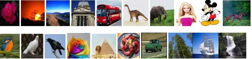
We have used database of 2000 bmp images for the experimentation. This includes 20 classes where each class contains 100 images of its own. The sample images from database are given in the Figure 4. This system is accepting the query as an example image. Each feature vector databases is tested with 200 randomly selected query images i.e ten images from each category.
3.2. Results and Discussion
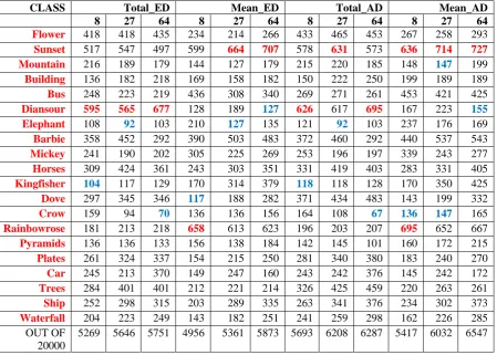
As per the above discussion we have feature vector databases for (Red_Count, Red_ Total and Red_Mean, similarly for green and blue color) three colors for each of the three sizes of feature vector that 8, 27 and 64. All these are tested using same set of query images so that all the approaches can be compared. Following tables are showing the results obtained for all these databases. Each entry in each of these columns is giving the retrieval of similar images out of 1000, which is total relevant retrieval images obtained for 10 queries of that particular class. We can observe that columns are classified as ED and AD which are actually discriminating the results obtained for two similarity measures Euclidean and Absolute distance respectively.
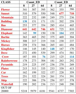
Table 1, 2 and 3 are showing the results for R, G, B colors respectively with Total and Mean intensities for 8, 27 and 64 bins. Table 4 is showing the results for count of pixels for all three sizes of bins. In these results we can observe that results based on similarity measure absolute distance is giving very good results for all three types of features that Count, Total and Mean as compared to the Euclidean distance. Comparing the results based on the types feature vectors it is found that ‘Count’ of pixels giving good similarity retrieval as compared to other two feature vectors. Between Total and Mean feature vector ‘Total’ of intensities are performing better as compared to ‘Mean’ of them. When the results compared on the basis of colors, percentage retrieval of similar images in red color is higher as compared to other two colors; it is around 60% for Red, 58% for green and 53% for Blue. Now if we observe the results on the basis of the dimensions of feature vectors that are 8, 27 and 64; feature vector of size 27 bins is proving its best in terms of the retrieval as compared to the 8 and 64 bins. We can say that it reduces the computation time of the system by reducing the no of bins as compared to 64 bins; and it captures more details about the color distribution of pixels as compared to 8 bins.
These results are analyzed and we have refined them using the three criteria named crtierion1, 2 and 3 so that the results can be narrowed and refined by combining them [29, 30]. Following charts are giving the results after applying these three criteria to combine the results obtained separately for three colors R, G and B.
Table 1. Results obtained for Red Plane with ED and AD for TOAL and MEAN feature vector Bins 8, 27, 64.
Table2: Results obtained for Green Plane with ED andAD for TOAL and MEAN feature vector Bins 8, 27, 64.
CLASS Total_ED Mean_ED Total_AD Mean_AD 8 27 64 8 27 64 8 27 64 8 27 64
Flower 418 418 435 234 214 266 433 465 453 267 258 293
Sunset 517 547 497 599 664 707 578 631 573 636 714 727
Mountain 216 189 179 144 127 179 215 220 185 148 147 199
Building 136 182 218 169 158 182 150 222 250 199 189 189
Bus 248 223 219 436 308 340 269 271 261 453 421 425
Diansour 595 565 677 128 189 127 626 617 695 167 223 155
Elephant 108 92 103 210 127 135 121 92 103 237 176 169
Barbie 358 452 292 390 503 483 372 460 292 440 537 543
Mickey 241 190 202 305 225 269 253 196 197 339 243 277
Horses 309 424 361 243 303 351 331 419 403 283 331 405
Kingfisher 104 117 129 170 314 379 118 118 128 170 350 425
Dove 297 345 346 117 188 282 371 434 483 143 199 332
Crow 159 94 70 136 136 156 164 108 67 136 147 165
Rainbowrose 181 213 218 658 613 623 196 203 207 695 652 667
Pyramids 136 136 133 156 138 184 142 145 101 160 172 215
Plates 261 324 337 154 215 250 281 340 380 183 240 270
Car 245 213 370 149 247 160 243 242 376 145 242 172
Trees 284 401 401 212 221 214 326 425 459 220 263 261
Ship 252 298 315 203 289 335 263 341 376 234 302 373
Waterfall 204 223 249 143 182 251 241 259 298 162 226 285
OUT OF 20000
5269 5646 5751 4956 5361 5873 5693 6208 6287 5417 6032 6547
CLASS Total_ED Mean_ED Total_AD Mean_AD 8 27 64 8 27 64 8 27 64 8 27 64
Flower 351 294 276 186 321 374 387 345 309 248 388 385
Sunset 534 538 472 648 707 711 536 581 508 709 764 744
Mountain 178 197 199 176 116 162 182 219 203 178 144 184
Building 143 205 273 126 165 186 155 241 309 156 177 199
Bus 295 353 307 282 474 477 326 368 343 282 512 511
Diansour 680 580 676 108 202 114 706 642 719 188 251 157
Elephant 145 106 113 225 128 164 152 102 117 250 157 181
Barbie 338 448 292 459 483 462 379 444 292 480 517 491
Mickey 282 193 205 308 308 301 299 191 198 366 305 296
Horses 279 462 431 158 230 328 299 484 472 234 285 384
Kingfisher 110 112 122 263 258 279 108 118 127 268 300 353
Dove 330 370 368 95 194 257 395 475 513 150 207 331
Crow 208 97 86 159 169 192 248 120 115 150 177 191
Rainbowrose 186 222 216 413 618 434 188 250 254 432 643 592
Pyramids 145 122 127 159 141 183 144 140 118 179 186 226
Plates 240 334 356 131 199 206 261 324 364 169 238 254
Car 182 200 366 184 111 89 197 237 376 174 134 106
Trees 248 427 461 232 239 239 296 468 488 239 283 274
Ship 293 354 368 275 276 289 290 422 453 297 327 342
Waterfall 208 235 258 218 214 228 258 267 305 241 281 287
OUT OF20000
Table 3. Results obtained for Blue Plane with ED and AD for TOAL and MEAN feature vector Bins 8, 27, 64.
Table 4: Results obtained with ED and AD for Count of Pixels in Bins 8, 27, 64.
CLASS Count_ED Count_ED 8 27 64 8 27 64
Flower 341 307 395 362 355 386
Sunset 510 579 550 548 677 710
Mountain 222 232 189 249 275 236
Building 138 151 171 151 202 259
Bus 253 377 354 285 414 465
Diansour 641 642 746 651 725 810
Elephant 142 99 150 138 104 155
Barbie 363 465 292 375 469 304
Mickey 308 217 219 318 230 237
Horses 258 374 366 265 441 484
Kingfisher 146 145 140 148 167 170
Dove 272 450 539 299 474 581
Crow 187 101 76 215 125 114
Rainbowrose 178 273 304 181 263 292
Pyramids 219 225 197 236 270 269
Plates 215 313 335 233 339 413
Car 162 199 322 157 228 359
Trees 251 322 324 261 374 391
Ship 222 306 276 256 357 378
Waterfall 190 202 236 213 248 290
OUT OF
20000 5218 5979 6181 5541 6737 7303
CLASS Total_ED Mean_ED Total_AD Mean_AD 8 27 64 8 27 64 8 27 64 8 27 64
Flower 342 297 313 236 340 360 347 352 339 267 313 267
Sunset 432 488 494 645 479 508 440 531 540 649 542 649
Mountain 217 199 158 144 156 195 225 209 158 157 173 157
Building 124 143 181 132 136 135 145 189 207 154 170 154
Bus 214 194 178 339 355 418 240 238 221 357 433 357
Diansour 545 580 692 131 188 117 580 623 731 177 233 177
Elephant 107 96 125 153 176 141 115 93 117 186 193 186
Barbie 365 447 292 400 395 426 369 444 292 446 476 446
Mickey 249 187 204 260 189 236 248 199 199 307 217 307
Horses 284 404 360 207 230 359 285 414 419 236 297 236
Kingfisher 87 115 94 184 332 329 91 118 106 186 337 186
Dove 272 336 363 112 178 237 332 398 440 149 201 149
Crow 168 88 68 87 96 117 180 101 62 128 127 128
Rainbowrose 162 151 148 537 635 613 155 159 142 503 642 503
Pyramids 155 184 150 122 113 146 174 167 94 122 165 122
Plates 230 280 289 178 204 240 259 304 326 209 234 209
Car 312 222 335 217 146 152 295 238 305 212 162 212
Trees 249 319 341 214 195 212 275 385 440 226 251 226
Ship 259 280 277 194 245 281 279 296 335 251 307 251
Waterfall 197 216 247 133 176 236 234 268 306 125 252 125
OUT
OF20000 4970 5226 5309 4625 4964 5458 5268 5726 5779 5047 5725 5047
Chart1. Combined Results of R, G and B colors using Criteria 1, 2 and 3 for 8 Bins.
Chart 2. Combined Results of R, G and B colors using Criteria 1, 2 and 3 for 27 Bins
When we observed these charts1, 2 and 3 for 8, 27 and 64 bins respectively, we can say that performance of 8 bins is poor among all three for both Total and Mean feature vectors with ED and AD. Bins 27 are giving better retrieval as compared to 8 Bins here both the results of Total and Mean with ED and AD are improved with quite good increment. 64 Bins have proved themselves by generating the results far better than 8 and 27 bins. In the chart 3 we can see that all columns are reached to very good height. These results are giving the cross over point (Precision and Recall) reached to 0.4. In case of Criteria 1, 2 and 3 in all three sizes of feature vectors, the performance is in increasing order as 1, 2 and 3, in short, Criterion 3 is giving best result among all three and Criterion 1 is giving poor results among them.
3.3. Performance Evaluation of the proposed Approaches
To evaluate the performance of the proposed approaches we have used two parameters that are LIRS- Length of
Initial Relevant String’ and ‘LSRR- Length of the String to Retrieve all Relevant images’. Results obtained using these parameters are plotted in charts 4, 5, 6 and 7. LIRS gives count of initial relevant string of the images obtained by giving the query, calculating the distance and sorting them in ascending order and LSRR is the length we need to travel the sorted distances between 1 to 2000, to retrieve all images relevant to the query. The results shown in charts are the average percentage of LIRS and LSRR for 10 queries from each of the 20 classes. When we evaluate the performance of the system in terms of LIRS and LSRR ideally, LIRS values should be as high as possible and LSRR should be as low as possible. In our approaches the best values of LIRS we obtained in few of the individual queries in the range from 60 to 77 which is very good achievement in these results. The best value of LSRR is 10% and worst value is 100%. and for the LIRS result the best value is 77 and worst value is 1.
Chart4. LIRS for 8 Bins with ED and AD
Chart 5. LSRR for 27 Bins with ED and AD
Chart 8. LIRS for 64 Bins with ED and AD Chart 9. LSRR for 64 Bins with ED and AD
Charts 4 - 5, 6-7, and Chart 8-9 are representing percentage retrieval obtained for LIRS and LSRR parameters for feature vectors Total, Mean and Count of size of 8, 27, 64 bins respectively.
In above results the best value obtained for LIRS is 10, for 64 bins shown in Chart 8. Second is 9 for 27 bins and 7 for 8 bins. Performance indicated by parameter LSRR is giving good result for bins 27, feature vector ‘Count’ that is to retrieve all the images in short to get the ideal recall value i.e. 1, we need to travel the length 68% only of the total 2000 images. Second better result for LSRR is 70% for ‘Total’ R, G colors with absolute distance.
Various factors are there through which the performance of this proposed system is evaluated
Types of Feature vectors: ‘ Count’, ‘Total’, Mean’ of R, G and B Intensities. Total of intensities are giving better results as compared to Count and Mean for all other factors mentioned below.
Sizes of Feature Vectors: 8 Bins, 27 Bins and 64 Bins: 8 bins performance is very pooras compared to 27 and 64 bins. Among all three bins considering both the distances, all three types of feature vectors and all three Criteria and LIRS LSRR values; we found that 64 Bins sizes are performing very well as compared to other two bins.
Combination and Refinement of R, G B plane’s Results using: Criterion 1, 2 and 3 : Refining and narrowing the results is achieved using these criteria, where,
Criterion 1 says that image will be retrieved in final set it it is being retrieved in all three.
Criterion 2 says that image will be retrieved in final set if it is being retrieved in any two of three planes.
Criterion 3 says that image will be retrieved in final set if it is being retrieved in atleast any one of the three planes.
They are giving the performance in increasing order of criterion1, 2 and 3. In brief Criterion 3 is doing best refinement and we could achieved very good results as average retrieval value is around 8000 out of 20, 000 ie. For total 200 queries.
Application of Similarity Measures: Euclidean Distance and Absolute Distance: Between these two, Absolute distance is proving itself by giving very good similarity retrieval as compared to Euclidean distance.
4. Conclusion
Content based image retrieval methods discussed in this paper are based on the 8, 27 and 64 Bins obtained by partitioning the equalized histogram into 2, 3 and 4 parts respectively. Partitioning has reduced the size of the histogram bins because of which we could reduce the computational complexity and save the processing time and still obtained better results. As discussed above system is evaluated for various different factors can be delineated in few words that among types of feature vector based on the contents extracted and represented ; ‘Count’ of pixels and their ‘Total intensities are performing better as compared to ‘Mean’
Among the three bins sizes overall performance of 64 bins is very good as compared to 8 and 27 bins sets. Among three colors Red color results are found dominating over green and blue. When these results are combined using the three criteria very good increase is obtained (8000 out of 20,000 i.e. Average for 200 queries) in the final retrieval of similar images; it indicates the precision recall cross over point is reached to 0.4. Absolute distance has done very good job as a similarity measure in our system by producing very good results for all the factors under consideration.
References
[1] Danqing Zhang, Binh Pham and Yuefeng Li,(2000) : Modelling Traditional Chinese Paintings for Content-Based Image
Classificationand Retrieval. Proceedings of the 10th International Multimedia Modelling Conference (MMM’04), 0-7695-2084-7/04 IEEE.
[2] Nidhi Singhai, Prof. Shishir K. Shandilya ( July 2010): A Survey On: Content Based Image Retrieval Systems , , International Journal
of Computer Applications (0975 – 8887)Volume 4 – No.2.
[3] Egon L. van den Broeka, Peter M. F. Kistersb, and Louis G. Vuurpijla (2000 )The utilization of human color categorization for
content-based image retrieval : http://www.icsi.berkeley.edu/wcs/
[4] Ying Liua, , Dengsheng Zhanga, Guojun Lua,Wei-Ying Mab,Y. Liu.(2007) : A survey of content-based image retrieval with
high-level semantics / Pattern Recognition 40 (2007) 262– 282.
[5] Xiaojun Qi,Yutao Han.(2005): A novel fusion approach to content-based image retrieval, www.sciencediretc.com
[6] Eduardo Valle, Matthieu Cord, Sylvie Philipp-Foliguet. CBIR in Cultural Databases for Identification of Images: A Local-Descriptors
Approach
[7] Zhang Lei, Lin Fuzong, Zhang Bo. (1999): A CBIR METHOD BASED ON COLOR-SPATIAL FEATURE . Proceeding of the IEEE
region 10 conference
[8] Ziqiang Feng and David Tien (2005) :Enhancement of Semantics in CBIR,Proceedings of the Third International Conference on
Information Technology and Applications (ICITA’05) 0-7695-2316-1/05IEEE.
[9] Muwei Jian, Junyu Dong, Ruichun Tang.(2007) : Combining Color, Texture And Region with Objects of User’s Interest for
Content-Based Image Retrieval ,0-7695-2909-7/07 2007 IEEE DOI 10.1109/SNPD.2007.104
[10] H. Wang, B. Chin, A. K.H. Tung. (2003): iSearch: Mining Retreival History for Content Based image retrieval. Proceedings of the
Eighth International Conference on Database Systems for Advanced Applications (DASFAA’03) 0-7695-1895/03, IEEE.
[11] Dong Kwon Park, Yoon Seok Jeon, Chee Sun Won, Soo-Jun Park, Seong-Joon Yoo. (2002): A Composite Histogram for Image
Retrieval. 6th August 2002 IEEE explore. Digital library.
[12] Neetu Sharma, Paresh Rawat,Jaikaran Singh.(2011): Efficient CBIR Using Color Histogram Processing, Signal & Image Processing :
An International Journal(SIPIJ) Vol.2, No.1, March 2011.
[13] Darshak G. Thakore, A. I. Trivedi. ( 2010) : Content based image retrieval techniques – Issues, analysis and the state of the art
[14] Remco C. Veltkamp, Mirela Tanase(2002) : Content-Based Image Retrieval Systems: A Survey. Survey report of around 62 pages on
different CBIR systems with features used, matching and evaluation.
[15] Guang Yang, Yingyuan Xiao. (2008) : A Robust Similarity Measure Method in CBIR System. 2008 Congress on Image and Signal
Processing 978-0-7695-3119-9/08 $25.00 © 2008 IEEE DOI 10.1109/CISP.2008.185 662 IEEE comp society.
[16] Ramadas Sudhir, Lt. Dr. S. Santhosh Baboo. (2011): An Efficient CBIR Technique with YUV Color Space and Texture Features,
Computer Engineering and Inteligent systems ISSN 2222-1719, -2863(OL),Vol 2, No. 6 2011
[17] P.S.Suhasini , 2dr. K.Sri Rama Krishna, 3dr. I. V. Murali Krishna. (2009) : Cbir Using Color Histogram Processing. Journal Of
Theoretical And Applied Information Technology© 2005 - 2009 Jatit. Www.Jatit.Org 13 Vol 6, No1.
[18] V. Vijaya Kumar, N. Gnaneswara Rao, A.L.Narsimha Rao, and V.Venkata Krishna.(2009) IHBM: Integrated Histogram Bin
Matching For Similarity Measures of Color Image Retrieval, Pattern recognition vol 2 issue 3 pages 109 -120
[19] Giung P. Nguyen and Marcel Worring. (2004) : optimizing similarity based visualization in Content based image retrieval. 2004 IEEE
International Conference on Multimedia and Expo (ICME).
[20] Aamer Mohamed, F. Khellfi, Ying Weng, and, Jianmin Jiang,Stan.Ipson.(2009) :An efficient Image Retrieval through DCT Histogram
Quantization. 2009 International Conference on CyberWorlds.
[21] N.K.Kamila, ,Pradeep Kumar Mallick, Sasmita Parida B.Das.(2010): Image Retrieval using Equalized Histogram Image Bins
Moments Special Issue of IJCCT Vol. 2 Issue 2, 3, 4; 2010 for International Conference [ICCT-2010], 3rd-5th December 2010.
[22] Chi-Man Pun*, Chan-Fong Wong. (2011) : Fast and Robust Color Feature Extraction for Content-based Image Retrieval, International
Journal of Advancements in Computing Technology Volume 3, Number 6, July 2011.
[23] A. Vadivel, A.K. Majumdar, Shamik Sural. (2003): Perceptually Smooth Histogram Generation from the HSV Color Space for
[24] Ole Andreas Flaaten Jonsgård.(2005): Improvements on colour histogram-based CBIR. Master’s Thesis ,Gjøvik University College.
[25] H. B. Kekre , Kavita Sonawane, “Feature Extraction in Bins Using Global and Local thresholding of Images for CBIR” International
Journal Of Computer Applications In Applications In Engineering, Technology And Sciences, ISSN: 0974-3596, October ’09 – March ’10, Volume 2 : Issue 2
[26] H. B. Kekre, Kavita Sonawane. (2012) : Bins Approach to Image retrieval using Statistical Parameters Based on Histogram
Partitioning of R, G, B Planes, IJAET, Jan 2012, ISSN 2231-196.
[27] H. B. Kekre, Kavita Patil. (2009) : Standard Deviation of Mean and Variance of Rows and Columns of Images for CBIR Standard
Deviation of Mean and Variance of Rows and Columns of Images for CBIR. International Journal of Computer, Information, and Systems Science, and Engineering (WASET).
[28] Dr. H. B. Kekre, Dhirendra Mishra “Image Retrieval using DST and DST Wavelet Sectorization”, (IJACSA) International Journal of
Advanced Computer Science and Applications, Vol. 2, No. 6, 2011.
[29] H. B. Kekre, Kavita Sonawane(2011) : Query based Image Retrieval using Kekre’s, DCT and Hybrid wavelet Transform over 1st and
2nd Moment, International Journal of Computer Applications (0975 – 8887),Volume 32– No.4, October 2011
[30] H. B. Kekre, Kavita Sonawane (2011): ‘Retrieval of Images Using DCT and DCT Wavelet Over Image Blocks” (IJACSA)
International Journal of Advanced Computer Science and Applications, Vol. 2, No. 10, 2011.
[31] H. B. Kekre, Kavita Patil.(2008) : DCT over Color Distribution of Rows and Columns of Image for CBIR. Sanshodhan – A Technical
Magazine of SFIT No. 4 pp. 45-51, Dec.2008.
[32] H. B. Kekre, Kavita Patil. WALSH Transform over color distribution of Rows and Columns of Images for CBIR. International
Conference on Content Based Image Retrieval (ICCBIR) PES Institute of Technology, Bangalore on 16-18 July 2008.
Dr. H. B. Kekre has received B.E. (Hons.) in Telecomm. Engg. from Jabalpur University in 1958,M.Tech (Industrial Electronics) from IIT Bombay in 1960, M.S. Engg. (Electrical Engg.) from University of Ottawa in 1965 and Ph.D. (System Identification) from IIT Bombay in 1970. He has worked Over 35 years as Faculty of Electrical Engineering and then HOD Computer Science and Engg. at IIT Bombay. For last 13 years worked as a Professor in Department of Computer Engg. at Thadomal Shahani Engineering College, Mumbai. He is currently Senior Professor working with Mukesh Patel School of Technology Management and Engineering, SVKM’s NMIMS University, Vile Parle(w), Mumbai, INDIA. He has guided 17 Ph.D.s, 150 M.E./M.Tech Projects and several B.E./B.Tech Projects. His areas of interest are Digital Signal processing, Image Processing and Computer Networks. He has more than 450 papers in National / International Conferences / Journals to his credit. Recently twelve students working under his guidance have received best paper awards. Five of his students have been awarded Ph. D. of NMIMS University. Currently he is guiding eight Ph.D. students. He is member of ISTE and IETE.
.She is member of ISTE. Ms. Kavita V. Sonawane has received M.E (Computer Engineering) degree from