www.nat-hazards-earth-syst-sci.net/16/1771/2016/ doi:10.5194/nhess-16-1771-2016
© Author(s) 2016. CC Attribution 3.0 License.
Vulnerability curves vs. vulnerability indicators: application
of an indicator-based methodology for debris-flow hazards
Maria Papathoma-Köhle
Institute of Mountain Risk Egineering, University of Natural Resources and Life Sciences, 1190 Vienna, Austria Correspondence to:Maria Papathoma-Köhle ([email protected])
Received: 7 March 2016 – Published in Nat. Hazards Earth Syst. Sci. Discuss.: 15 March 2016 Revised: 2 June 2016 – Accepted: 1 July 2016 – Published: 3 August 2016
Abstract.The assessment of the physical vulnerability of el-ements at risk as part of the risk analysis is an essential as-pect for the development of strategies and structural mea-sures for risk reduction. Understanding, analysing and, if possible, quantifying physical vulnerability is a prerequisite for designing strategies and adopting tools for its reduction. The most common methods for assessing physical vulner-ability are vulnervulner-ability matrices, vulnervulner-ability curves and vulnerability indicators; however, in most of the cases, these methods are used in a conflicting way rather than in com-bination. The article focuses on two of these methods: vul-nerability curves and vulvul-nerability indicators. Vulvul-nerability curves express physical vulnerability as a function of the in-tensity of the process and the degree of loss, considering, in individual cases only, some structural characteristics of the affected buildings. However, a considerable amount of stud-ies argue that vulnerability assessment should focus on the identification of these variables that influence the vulnera-bility of an element at risk (vulneravulnera-bility indicators). In this study, an indicator-based methodology (IBM) for mountain hazards including debris flow (Kappes et al., 2012) is ap-plied to a case study for debris flows in South Tyrol, where in the past a vulnerability curve has been developed. The relatively “new” indicator-based method is being scrutinised and recommendations for its improvement are outlined. The comparison of the two methodological approaches and their results is challenging since both methodological approaches deal with vulnerability in a different way. However, it is still possible to highlight their weaknesses and strengths, show clearly that both methodologies are necessary for the as-sessment of physical vulnerability and provide a preliminary “holistic methodological framework” for physical
vulnera-bility assessment showing how the two approaches may be used in combination in the future.
1 Introduction
this point, the difference between fragility curves and vul-nerability curves has to be highlighted. Fragility curves ex-press the probability that a building will be damaged as a function of the intensity of the process, whereas vulnerabil-ity curves relate the intensvulnerabil-ity with the corresponding degree of loss. HAZUS, for example, defines five damage states for buildings subject to earthquake hazard (none, slight, moder-ate, extensive and complete) and develops fragility curves for different building types (HAZUS, 2006). HAZUS fragility curves present the probability for these five damage states to occur under different peak ground acceleration (PGA) val-ues (HAZUS, 2006). Nevertheless, vulnerability curves for different types of buildings may also be found in the litera-ture for earthquake, wind and flood hazards. In the present study an indicator-based methodology (IBM) is applied in Martell (South Tyrol, Italy) for debris flows. The same case study area has been used in the past for the development of a vulnerability curve based on damage data from a debris flow event in 1987 (Papathoma-Köhle et al., 2012). By com-paring the results of the two methods, the advantages and disadvantages of the IBM can be highlighted and recommen-dations for its further development and improvement can be outlined. Last but not least, a preliminary framework propos-ing the combination of these methods may be proposed.
2 Physical vulnerability assessment: the PTVA method and the use of indicators
Due to the multi-dimensional nature of vulnerability a long list of definitions can be found in the literature varying from general ones to more dimension-specific ones. As far as the physical vulnerability is concerned, the definition of UN-DRO (1984) (“vulnerability is the degree of loss to a given element, or set of elements, within the area affected by a haz-ard. It is expressed on a scale of 0 (no loss) to 1 (total loss)”) is in conflict with other, more general, definitions presenting vulnerability as susceptibility to harm or the result of a com-bination of characteristics of the elements at risk. For exam-ple, according to (UNISDR, 2009) vulnerability is defined as “the characteristics and circumstances of a community, sys-tem or asset that makes it susceptible to the damaging effects of a hazard”, often used by social scientists to describe the social dimension of vulnerability. The first definition is based on the ex post outcome of a specific event, whereas, the sec-ond is based on the ex ante csec-ondition of the elements at risk without considering the intensity or the characteristics of the hazardous process. From these two definitions various ap-proaches for vulnerability assessment derive that require dif-ferent datasets leading to diverse results. It is, therefore, clear that the lack of common definition for vulnerability results to the absence of a universal methodology for its assessment.
how-ever, it is relatively uncomplicated to develop reliable vul-nerability curves due to sufficient data availability. For other hazard types, such as rock falls, this is not the case since a single event affects only a limited amount of elements at risk and the assessment of the process intensity on each of them is a challenging process. Moreover, vulnerability curves do not consider the individual features of the buildings or char-acteristics related to their location and surroundings (Fuchs, 2009). Although they provide concrete information regard-ing the loss, they do not provide information concernregard-ing the drivers of vulnerability or potential ways of reducing it.
As far as debris flow is concerned, the first approaches for physical vulnerability assessment were qualitative (Fell and Hartford, 1997; Liu and Lei, 2003; Romang, 2004), includ-ing in some cases vulnerability matrices (Leone et al., 1995, 1996; Sterlacchini et al., 2007; Zanchetta et al., 2004) show-ing a descriptive relationship between the damage and inten-sity of the flow. However, recently the number of vulnera-bility curves for debris flows has considerably increased and several studies may be found in the literature (Fuchs et al., 2007; Papathoma-Köhle et al., 2012; Quan Luna et al., 2011; Totschnig and Fuchs, 2013; Totschnig et al., 2011). Each vul-nerability curve has been developed for a specific area, is based on a particular catastrophic event and expresses the in-tensity of the process in various ways. For example, there are curves based on data for a small (e.g. 13 buildings in Fuchs et al., 2007) or a larger number of buildings (1560 buildings in Lo et al., 2012). In some cases, due to lack of empirical data, information on the process had to be derived through modelling (Quan Luna et al., 2011; Rheinberger et al., 2013) that expressed the flow not only as debris height but also as velocity, viscosity or impact pressure. As far as the degree of loss is concerned, relevant information could be provided in some cases by the authorities. Nevertheless, where damage data were not available, damage costs were assessed based on photographic documentation (e.g. Papathoma-Köhle et al., 2012). Last but not least, it is worth mentioning that a num-ber of studies focus on laboratory experiments in order to determine the interaction between the flow and the structural components of the buildings (Gems et al., 2016; Zhang et al., 2016).
In contrast, shortage of empirical data often leads to the development of vulnerability indices based on the selection, weighting and aggregation of vulnerability indicators. IBMs have been used mainly for other vulnerability dimensions, such as social or economic vulnerability. However, recently a considerable number of studies are available that make use of vulnerability indicators for the assessment of other vulner-ability dimensions (e.g. physical). Vulnervulner-ability indicators, according to Birkmann (2006), are “variables which are op-eration representations of a characteristic quality of the sys-tem able to provide information regarding the susceptibility, coping capacity and resilience of a system to an impact of an albeit ill-defined event linked to a hazard of a natural origin”. The importance of developing and using indicators has been
Last but not least, Kappes et al. (2012) developed an IBM for multi-hazard in mountain areas which is presented in de-tail and applied in the present study. In general, in most of the studies, indicators are weighted empirically and no vali-dation of their selection and weighting has been implemented using the damage pattern and loss from a real event. 2.2 The PTVA method and its evolution
One of the first attempts to use indicators for the assess-ment of physical vulnerability was made by Papathoma and Dominey-Howes (2003) and Papathoma et al. (2003). Specif-ically, they developed a methodology for assessing the phys-ical vulnerability of buildings to tsunami at coastal areas in Greece using indicators. The main concept of the Papathoma Tsunami Vulnerability Assessment Model (PTVA) was the combination of an inundation scenario with “attributes relat-ing to the design, condition and surroundrelat-ings of the build-ing” (Tarbotton et al., 2012). The methodology was based on the fact that two buildings located exactly at the same place despite experiencing the same process intensity do not always suffer the same loss. The reason for this is the va-riety of building characteristics concerning the building it-self and its surroundings. A number of buildings charac-teristics related to the damage pattern following a tsunami event were selected (indicators) and a GIS database with the buildings and their attributes was created. The indicators were weighted using expert judgement and a vulnerability index was given to each building. The result was a series of maps for a number of coastal segments in Greece show-ing the spatial pattern of the relative physical vulnerability of the buildings. In this way, authorities and emergency ser-vices could focus their limited resources on specific build-ings rather the whole potentially inundated area. The method was later validated (Dominey-Howes and Papathoma, 2007) using data from Maldives following the 2004 Indian Ocean tsunami. The validation showed that the selected vulnerabil-ity indicators correlate well with the severvulnerabil-ity of the damage; however, recommendations for improvement led to an im-proved version of the method: PTVA-2. PTVA-2 was used in the USA (Dominey-Howes et al., 2010) for the estima-tion of the probable maximum loss from a Cascadia tsunami in Oregon (USA). The main difference to PTVA-1 was the inclusion of the water depth above ground as an attribute in the calculation of the overall vulnerability. In this way, the method became more intensity dependant than before. PTVA-3 was developed by Dall’Osso et al. (2009a) and was tested in Australia (Dall’Osso et al., 2009b) and in Italy (Dall’Osso et al., 2010). PTVA-3 made a step towards and more reliable weighting of the vulnerability indicators by using analytical hierarchy process (AHP) rather than expert judgement to weight the attributes.
The first attempt to use vulnerability indicators for moun-tain hazards was made by Papathoma-Köhle et al. (2007) with the development of an elements at risk database
contain-ing indicators regardcontain-ing the physical vulnerability of build-ings to landslides. However, due to the lack of data regard-ing the hazardous process itself and the limited availability of data regarding the building characteristics the study con-stitutes only a good basis for further research. The next at-tempt was made by Kappes et al. (2012), who introduced a methodology for vulnerability assessment using vulnera-bility indicators, e.g. characteristics of the building that are responsible for its susceptibility to damage and loss due to mountain hazards, based on the PTVA model. The method-ology is presented in the following chapter. It is clear that as far as mountain hazards are concerned, there is definitely a need to improve and modify indicator-based approaches in order to be used for vulnerability assessment and as basis for risk reduction strategies.
The two methodological concepts have been always used separately rather than in combination from scientists and practitioners. A first effort to combine them has been made by Papathoma-Köhle et al. (2015). Papathoma-Köhle et al. (2015) developed a tool which uses the vulnerability curve presented in the following chapters as a core to implement three functions: updating and improvement of the curve with data from new events, damage and loss assessment for future events and damage documentation of new events. However, the tool has the possibility to include information regarding building characteristics. This provides the opportunity to in-vestigate the correlation of damage patterns and the building characteristics in the future.
3 The indicator-based methodology: a PTVA for debris flow
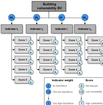
The concept of the IBM for mountain hazards (debris flows, landslides and floods) is based on the assignment of weights to a number of building characteristics resulting to a relative vulnerability index (RVI) per building (Fig. 1). The RVI is calculated per building by using the following Eq. (1): RVI=
m X
1
wm·Imsn, (1)
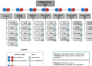
wherewrepresents themdifferent weights,I them indica-tors andsthenscores of the indicators as shown in Fig. 1. A selection of vulnerability indicators of buildings for debris flow events and the weighting according to different users are shown in Fig. 2. In more detail, the vulnerability indica-tors are related to building characteristics (material, condi-tion, number of floors, building surroundings) and location (row towards torrent and row towards the slope). The indi-cators are weighted and aggregated according to Eq. (1) to a RVI which is attributed to each building.
Figure 1.The concept of the IBM (Kappes et al., 2012).
need to know the physical vulnerability of the buildings in or-der to locate concentrated number of casualties and potential victims following an event. Therefore, one-floor buildings not offering vertical evacuation opportunities are of greater importance. “Vertical evacuation” refers often to any action aiming at moving people to a higher area (higher ground, upper floors of multi-storey building or a vertical shelter) (Velotti et al., 2013) and is growing in importance in the Netherlands as an emergency management option for floods (Velotti et al., 2013), whereas in Japan it is already used for tsunamis (Scheer et al., 2011). However, if the aim of the study is the development of vulnerability reduction efforts during the preparedness phase, building material and condi-tion or the existence of building surroundings are of the high-est importance. In this way, several RVIs may be calculated for each building by varying scores and weights: for exam-ple, an RVIEPwhich can be used for emergency planning or
an RVIVRwhich can be used as a base for vulnerability
re-duction strategies (e.g. reinforcement of buildings).
Kappes et al. (2012) suggest that the main advantage of the method is the flexibility in weighting, although flexibil-ity in this case increases subjectivflexibil-ity, which consequently
accu-Figure 2.The IBM adapted for debris flow. The vulnerability indicators are demonstrated together with the weight index, which varies according to the objective of the vulnerability assessment and the end users (Kappes et al., 2012).
mulation of movable objects or even additional elements at risk, such as agricultural spaces and industry, will make the method more integrated. Furthermore, the database could be enriched with socioeconomic data at building level. Last but not least, Kappes et al. (2012) suggest that an interesting de-velopment of the method would be the validation of the indi-cators weighting based on damage records of past events.
The weighting of the indicators has been done without car-rying out a sensitivity analysis. A sensitivity analysis would be an important next step following the development of the IBM methodology of Kappes et al. (2012). A sensitivity analysis would show the different outcomes of the method by changing each time the assumptions – for example, the weighting of the indicators.
4 The case study area
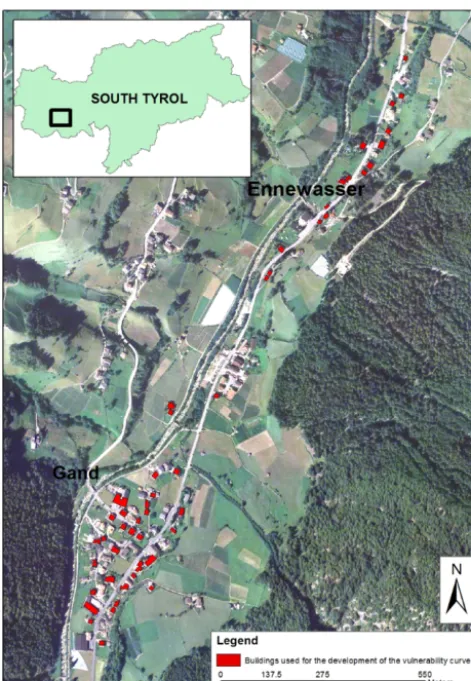
The IBM has to be tested in an area that has not only a long record of debris flow events but also detailed docu-mented damages on buildings. Damage documentation may additionally reveal information regarding the intensity of the event itself as well as the damage pattern on the built envi-ronment. For this reason, the methodology will be validated in Martell (South Tyrol, Italy). Communities in South Ty-rol (Italy) often suffered material damages due to
geomor-phological hazards such as landslides, flash floods and debris flows.
The municipality of Martell is located in the tributary val-ley of Vinschgau in South Tyrol, Italy. The valval-ley of Martell is 27km long with a ranging altitude from 950 to 3700 m (Martell, 2013). The settlements are located at the bottom of the valley which is mainly used for agriculture. Most of the built-up areas, such as Meiern, Gand, Ennewasser, and Burgaun are situated in the north part of the valley. Martell has a long record of water-related natural hazard events such as glacial lake outburst, floods, debris flows and avalanches. The loose material (debris) that was left behind by glaciers during the Holocene retreat has often been transported down-stream by debris flows in the past, causing considerable ma-terial damage to the settlements of the valley. Additionally, a reservoir dam was constructed in 1956, which served mainly as an electrical power source and protected the village from unexpected excessive flooding.
con-sidered as entirely natural, as it was directly connected to the mismanagement of the reservoir dam which failed to regu-late the water flow into the valley (Pfitscher, 1996). The ac-tual outflow has been estimated to be 3 times the usual dis-charge (300 to 350 m3s−1). The debris flow reached the vil-lage of Gand, overflowed the river bed and found its way through the settlements. Not only were buildings destroyed, but significant damages were also recorded in agricultural areas, infrastructure and the industrial zone in Vinschgau (Pfitscher, 1996). Fortunately, due to the early warning and evacuation no casualties were recorded. Although the total damage summed up to ITL 45 to 50 billion (approximately EUR 23.2 to 25.8 million), private households suffered dam-ages of slightly less than EUR 8 million.
As far as the infrastructure, local light industry, forestry, agriculture, tourism and emergency response are concerned, damages up to EUR 4 million were recorded. Furthermore, EUR 5.6 million had to be spent for the recovery of the re-gional road and the telecommunications network as well as for torrent control measures. At the time, only the direct costs of the event were assessed (Pfitscher, 1996). The event was documented mainly through photographic material (Fig. 4) that enabled later assessment of the intensity of the process as well as the damage pattern on individual buildings.
5 The development of a vulnerability curve for the study area
Following an intensive workshop with stakeholders from South Tyrol a methodology for developing a vulnerability curve for the area was created based on the needs of the stake-holders, their experience and the available data. The pilot study included the making of a vulnerability curve based on empirical damage data of buildings in Martell, South Tyrol, Italy, that were damaged during the 1987 debris flow event (Fig. 5). Following the event, the buildings, as well as parts of the affected villages, were photographed. These photographs give a very good overview of the damage pattern; however, information regarding the costs of the damages per building, or detailed descriptions of the damage, were not available. In more detail, photographic documentation of 51 buildings out of the 69 buildings that were damaged or completely de-stroyed during the event was used (Pfitscher, 1996), because only for this number of buildings was adequate photographic documentation available. Based on these photos, the height of the debris deposits per building could be estimated and the monetary damage was calculated. For example, in case the damage is limited to the exterior of the building, the works will include only restoration of the external walls. In case the debris has entered the building through openings or wall breaks, there will be additional renovation works such as re-moval of debris and restoration of interior walls and floor (Papathoma-Köhle et al., 2012). The extent of the damage per building was translated in monetary loss based on
stan-dard prices for renovation works (Kaswalder, 2009). By com-paring the value of a building in terms of reconstruction costs to the monetary damage caused by the event the degree of loss per building could be also assessed. Every building used in the analysis was represented as a point in thexyaxis sys-tem shown in Fig. 5. A Weibull function was fitted to the data points as this curve was the one that fulfilled the defined cri-teria (the curve has to go through 0 and not over degree of loss 1) and had the bestR2(coefficient of determination).
The vulnerability curve clearly shows that the higher the intensity of the process the greater the damage that an ele-ment at risk suffers. The curve indicates that when the in-tensity exceeds 1.5 m, the degree of loss increases consid-erably. This may be explained by the fact that debris flow of this height may easily enter the building from windows and doors and cause additional damage in the interior. How-ever, at this point it is important to emphasise that only the structural damage was considered in the calculation of the monetary loss and not the content of the buildings. In more detail, the costs of the structural damage included cleaning up of the interior, repairing the exterior and interior walls, removing and replacing doors and windows, and testing and reinstalling electric, heating and sewage systems where nec-essary.
Finally, Papathoma-Köhle et al. (2012) computed a vali-dation curve (blue curve in Fig. 3) using real compensation data for only part of the buildings provided by the Depart-ment of Domestic Construction of the Autonomous Province of Bozen/Bolzano for the calculation of the degree of loss. The visual comparison of the two curves demonstrated the validity of the vulnerability curve.
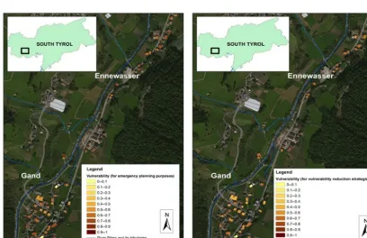
The results (intensity and degree of loss) are displayed herein for the first time in two separate maps (Fig. 6) in or-der to demonstrate the spatial pattern of the two factors. By the maps it is clear that buildings located very close to the steep slope experienced higher intensity. For buildings situ-ated next to the road also high intensity values were recorded, probably because roads acted as preferred corridors that en-abled the debris flow to enter the settlement area. Moreover, in Fig. 6 is also obvious that in Ennewasser (north of the map) the intensities were significantly lower due to the pro-tection offered by the forest on the east side of the settlement. In Fig. 6 (right map) the spatial distribution of the degree of loss follows in most cases the pattern of the intensity distri-bution. Table 1 clearly shows that the majority of the build-ings experienced rather low intensity of debris flow (less than 1m debris height). Only nine buildings (17.5 %) experienced high intensity of debris flow (more than 2 m debris height).
Figure 3.The case study area: municipality of Martell (villages of Gand and Ennewasser). The buildings used in the case study are highlighted in red colour.
direction. The vulnerability curve also shows that there are buildings (points) that, although they have experienced low intensities, have suffered a considerable degree of loss. This may be explained by the existence of basements or of base-ment windows that allowed material to enter the basebase-ment and cause additional damage to the building. However, the opposite phenomenon may be also observed. There are build-ings that although they have experienced very high intensity, the degree of loss is relatively low. Since the degree of loss is a percentage of loss, buildings with more than one floor will experience a lower degree of loss as percentage of their over-all value. This shows the importance of indicators concerning the number of floors or the height of the building.
6 The application of the IBM in the study area
The IBM was applied at the same buildings that were used for the computation of the vulnerability curve in Gand and En-newasser (Municipality of Martell). Based on photographic documentation provided from the municipality of Martell a
Table 1.Intensity categories and the corresponding number of af-fected buildings.
Intensity Number of %
buildings
<1 30 59
1–2 12 23.5
>2 9 17.5
Figure 4.Example of photographic documentation following the August 1987 event (source: municipality of Martell).
Figure 5.The vulnerability curve and the validation curve based on damage data from the 1987 debris flow event in Martell (South Tyrol) (Papathoma-Köhle et al., 2012).
Figure 6.The spatial pattern of the assessed intensity of the 1987 event per building (left panel) and the corresponding degree of loss (right panel) in the villages Gand and Ennewasser.
have been assessed and calculated respectively during the de-velopment of the vulnerability curve (Papathoma-Köhle et al., 2012).
The vulnerability indicators were collected for each build-ing, and as shown in the example of Fig. 7, RVIEPand RVIVR
were calculated. The RVIEP is a relative vulnerability
in-dex that is important for professionals designing emergency evacuation plans. This may include local authorities or emer-gency services such as the fire brigade. The RVIVR is a
rel-ative vulnerability index that may indicate the buildings that need reinforcement or local protection measures in order to reduce their physical vulnerability to debris flow. This infor-mation may interest local authorities and individual building owners but also insurance companies. The application of the RVI at Martell shows that the weighting of the vulnerability indicators by different end users leads (at least in this case) to rather similar results (Figs. 8 and 9 and Table 2) and that differences are focused on individual buildings.
In the following paragraphs the results of the two meth-ods are compared, the benefits and drawbacks of the indica-tors based method are listed and improvements not only for the further development of IBMs but also for the improve-ment of the assessimprove-ment of physical vulnerability in general are outlined.
7 Results and discussion
7.1 Comparison of the results of both methods
The spatial distribution of damage and intensity data used for the development of vulnerability curves is not often dis-played on a map, although this would be simple with the use of GIS. The curves are mainly used as a tool that displays geographically distributed information on axy axis system and may predict the degree of loss of a building should it experience a specific intensity. However, in the present arti-cle the spatial pattern of the intensity and the degree of loss are displayed in two maps in Fig. 6. The comparison of the results of the IBM (Fig. 8) with the intensity of the process per building of the 1987 event and the spatial distribution of the degree of loss (Fig. 6) (Papathoma-Köhle et al., 2012) shows that the results of both methods are generally com-patible. The buildings that experienced a high degree of loss (Fig. 6) are often the ones with a high RVI, especially in the case of RVIVR. However, the visual comparison of the maps
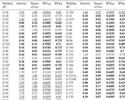
regard-Table 2.Comparison of the results per building. The typeface indicates the degree of intensity as described in Table 1 (bold for
inten-sity<1 m, italic for intensities 1–2 m and underlined for intensities>2 m).
Building Intensity Degree RVIVR RVIEP Building Intensity Degree RVIVR RVIEP
ID of loss ID of loss
G 26 2.10 1.00 0.6565 0.88 G 226 2.40 0.22 0.5055 0.565
G 28 1.20 0.10 0.6285 0.735 G 41 0.10 0.04 0.4335 0.53
G 29 2.40 1.00 0.6615 0.76 G 219 0.10 0.02 0.5305 0.55
G 30 0.80 0.10 0.5885 0.665 G 42 0.10 0.02 0.4305 0.51 G 32 2.50 0.71 0.6135 0.69 G 45 0.20 0.05 0.4665 0.56 G 35 1.90 1.00 0.6285 0.735 G 46 0.30 0.06 0.5605 0.62 G 36 0.20 0.07 0.5855 0.645 G 60 0.20 0.01 0.5335 0.61 G 37 0.60 0.07 0.5855 0.645 G 62 0.10 0.03 0.6035 0.64 G 38 0.10 0.00 0.6815 0.735 M 68 0.10 0.05 0.6755 0.695
G 224 1.60 0.32 0.5985 0.71 M 69 0.10 0.01 0.6945 0.805
G 47 0.10 0.01 0.6785 0.715 E 148 0.50 0.01 0.6755 0.74 G 48 0.10 0.01 0.6315 0.755 E 153 0.10 0.01 0.6485 0.7 G 49 0.10 0.01 0.6215 0.705 E 154 1.30 0.31 0.6755 0.74 G 55 1.10 0.24 0.6945 0.805 E 157 0.10 0.01 0.5845 0.655 G 54 0.20 0.04 0.5905 0.65 E 159 0.20 0.01 0.6355 0.765
G 225 0.10 0.01 0.6855 0.745 E 160 0.30 0.01 0.6855 0.745
G 52 1.00 0.19 0.5565 0.65 E 161 1.00 0.12 0.6755 0.695 G 53 1.70 0.27 0.5145 0.625 E 162 0.40 0.08 0.6455 0.68
G 56 3.00 1.00 0.5785 0.615 E 221/A 0.20 0.09 0.6885 0.765
G 57 1.20 0.24 0.4885 0.565 E 221/B 0.20 0.05 0.6755 0.695
G 59 2.50 1.00 0.6685 0.745 E 170 0.80 0.07 0.5385 0.635
G 58 2.50 1.00 0.5785 0.615 E 171 0.70 0.17 0.6885 0.765
G 66 2.10 0.40 0.5785 0.615 E 172 1.00 0.10 0.6755 0.695
G 65 1.30 0.13 0.6085 0.685 E 173 0.40 0.03 0.6655 0.69
G 64 2.20 0.55 0.5035 0.54 E 176 0.10 0.07 0.6585 0.75
G 63 1.20 0.13 0.4885 0.585
ing the intensity. It is clear that the two approaches define vulnerability in a different way, namely as a result of intrin-sic characteristics in one case (IBM) or as a consequence of a specific hazard intensity in the other (vulnerability curves). In contrast, there are buildings in Gand that, although they have experienced a high degree of loss, are assigned with a low RVI. The high degree of loss is expected since, accord-ing to Fig. 6, the same buildaccord-ing also experienced high inten-sity. It is, therefore, clear that the results show inconsistencies because the intensity is not considered by the IBM. Never-theless, some vulnerability indicators are directly connected to the intensity that a building experiences, e.g. surrounding vegetation or protection from other buildings or proximity to the road network.
By visualising the spatial pattern of the degree of loss and the observed intensity, as well as their relationship through vulnerability curves, additional valuable information regard-ing the importance of vulnerability indicators may become available and, in this way, the IBM may be modified, ex-tended and substantially improved. For example, the low in-tensities recorded on buildings in Ennewasser may be related to the presence of surrounding vegetation, which highlights the importance of the relevant vulnerability indicator. This
leads to the conclusion that both methods, although based on a different concept, shed light on two different aspects of the physical vulnerability: specifically, the intrinsic characteris-tics of the buildings and the expected degree of loss under a given intensity respectively; therefore, they should be used in combination rather than in conflict. Apart from the visual comparison of the results, a closer look to the results for each building in Table 2 reveals even more about the advantages and disadvantage of both methods.
In Table 2 the results of both methods are displayed for each of the 51 buildings of the case study. The comparison of the results leads to a number of interesting observations.
1. The RVI values vary from 0.43 to 0.88. No extreme val-ues are observed. There are no buildings with RVI=1. This is to be expected since there are no buildings in the area with extreme scores (e.g. material=wood or con-dition=ruin).
Figure 7.An example of the application of the IBM for two different objectives: for evacuation planning (RVIEP) and for vulnerability
reduction strategies and reinforcement (RVIVR).
under investigation are located within the area affected by the debris flow. This is also supported by the vulner-ability curve, which is based on a real event and shows that no building suffered 0 degrees of loss.
3. As far as the comparison between the two methodolo-gies is concerned, some buildings, although they experi-enced low degree of loss, are assigned a high RVI. This can be explained by the fact that the IBM is not intensity specific. The high RVI means that the specific build-ing could experience a high degree of loss due to its characteristics. However, the vulnerability curve shows that the specific building did not suffer a high degree of loss during the event for reasons that may be con-nected to characteristics of the process itself (e.g. G48). This is even more obvious in the case of buildings G53 and G56. The two buildings have been assigned with similar RVIs. They have, however, experienced degrees of loss of 1 and 0.27 respectively. This is explained by the significant difference in the process intensity (1.7 and 3 m respectively).
4. However, the contrary observation is also evident: some buildings have been impacted by debris flow of high in-tensity which resulted in a low degree of loss (e.g. G53, G64, G66, G224, G226). Obviously, the fact that build-ings, although they experience the same intensity of the process, experience different degrees of loss (some are completely destroyed and some others have less than 50 % of loss) may be explained by significant differ-ences in their attributes. However, another explanation may be related to characteristics of the process that are not considered by the vulnerability curve, such as veloc-ity of the flow, direction of impact, viscosveloc-ity, duration, size of debris, etc.
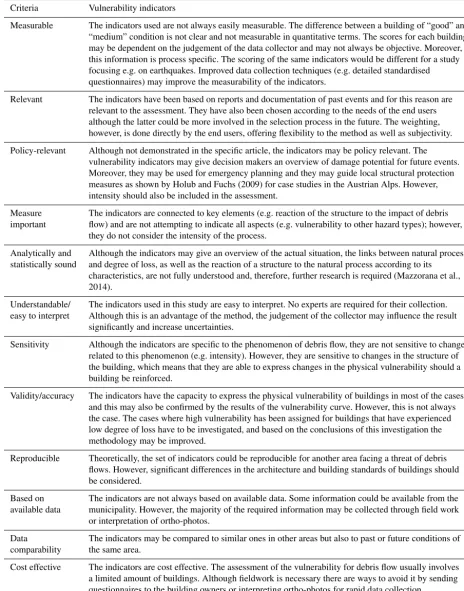
The results of the IBM depend on the set of indicators used for the calculation of the RVI. The IBM is based on a set of indicators that were selected based on expert judge-ment, damage reports and photographic documentation of past events. However, Birkmann (2006), based on existing sets of indicators (EEA, NZ Statistics etc.), provides a list of the quality criteria that vulnerability indicators have to fulfil. In Table 3 the set of indicators of the present study is tested towards some of these criteria.
Table 3 shows that although the set of indicators fulfils many criteria, there is still room for improvement of the indi-cator set itself, the description and assignment of the scores for each indicator and the collection of the required data. 7.2 Benefits, limitations and future development of the
IBM
In contrast to the vulnerability curves, IBMs are not estab-lished and applied by practitioners in the same dimension. For this reason, the comparison between the two concepts is
not only essential but also very challenging due to the differ-ent way that they approach vulnerability. However, this com-parison may highlight the benefits of the IBMs, point out its weaknesses and lead to a list of recommendations not only for the improvement of the indicator-based concept but also for the improvement of the assessment of physical vulnera-bility in the future.
The comparison of the two methods highlighted the fol-lowing benefits of using indicators for assessing physical vul-nerability of buildings to torrential hazards.
1. Contrary to vulnerability curves, the IBM prompts the user to develop aninventory of the elements at riskand a database of building characteristics. This may enable the development of strategies for the reduction of vul-nerability at a very local level, as well as the devel-opment of local structural protection measures. In this way, the focus and the resources will be concentrated on limited amount of buildings.
2. The IBM does not use empirical loss data but rather in-dicates therelative vulnerabilityof individual buildings. This means that this type of methodology can be ap-plied to areas with no recorded history of events, mak-ing its use possible in the absence of damage data. In other words, although the IBM does not have a predic-tive power in quantifying expected loss in comparison to the vulnerability curves, it does still have a predic-tive power in indicating the specific buildings that will experience loss.
3. The weighting is flexible and may be adjusted to the needs of individual users. This ensures the use of the methodology by a range of end users.
4. No expertsare required for the data collection. The as-signment of the scores of the individual indicators do not require any expert knowledge. This means that even the owners of the buildings may provide the required information themselves, saving in this way money and time for data collection.
5. The use of GIS makes theupdating of information eas-ier but, by changing the scores of indicators, we can also answer “what if” questions related to local struc-tural protection and reinforcement of buildings. The weights and scores may be fine-tuned by using informa-tion of past events. Moreover, by using easy to update databases future changes in the spatial pattern of the built environment, socioeconomic and land use changes may be considered for future scenarios.
Table 3.Quality criteria for vulnerability indicators (adapted from Birkmann, 2006).
Criteria Vulnerability indicators
Measurable The indicators used are not always easily measurable. The difference between a building of “good” and
“medium” condition is not clear and not measurable in quantitative terms. The scores for each building may be dependent on the judgement of the data collector and may not always be objective. Moreover, this information is process specific. The scoring of the same indicators would be different for a study focusing e.g. on earthquakes. Improved data collection techniques (e.g. detailed standardised questionnaires) may improve the measurability of the indicators.
Relevant The indicators have been based on reports and documentation of past events and for this reason are
relevant to the assessment. They have also been chosen according to the needs of the end users although the latter could be more involved in the selection process in the future. The weighting, however, is done directly by the end users, offering flexibility to the method as well as subjectivity.
Policy-relevant Although not demonstrated in the specific article, the indicators may be policy relevant. The
vulnerability indicators may give decision makers an overview of damage potential for future events. Moreover, they may be used for emergency planning and they may guide local structural protection measures as shown by Holub and Fuchs (2009) for case studies in the Austrian Alps. However, intensity should also be included in the assessment.
Measure The indicators are connected to key elements (e.g. reaction of the structure to the impact of debris
important flow) and are not attempting to indicate all aspects (e.g. vulnerability to other hazard types); however,
they do not consider the intensity of the process.
Analytically and Although the indicators may give an overview of the actual situation, the links between natural process
statistically sound and degree of loss, as well as the reaction of a structure to the natural process according to its
characteristics, are not fully understood and, therefore, further research is required (Mazzorana et al., 2014).
Understandable/ The indicators used in this study are easy to interpret. No experts are required for their collection.
easy to interpret Although this is an advantage of the method, the judgement of the collector may influence the result
significantly and increase uncertainties.
Sensitivity Although the indicators are specific to the phenomenon of debris flow, they are not sensitive to changes
related to this phenomenon (e.g. intensity). However, they are sensitive to changes in the structure of the building, which means that they are able to express changes in the physical vulnerability should a building be reinforced.
Validity/accuracy The indicators have the capacity to express the physical vulnerability of buildings in most of the cases
and this may also be confirmed by the results of the vulnerability curve. However, this is not always the case. The cases where high vulnerability has been assigned for buildings that have experienced low degree of loss have to be investigated, and based on the conclusions of this investigation the methodology may be improved.
Reproducible Theoretically, the set of indicators could be reproducible for another area facing a threat of debris
flows. However, significant differences in the architecture and building standards of buildings should be considered.
Based on The indicators are not always based on available data. Some information could be available from the
available data municipality. However, the majority of the required information may be collected through field work
or interpretation of ortho-photos.
Data The indicators may be compared to similar ones in other areas but also to past or future conditions of
comparability the same area.
Cost effective The indicators are cost effective. The assessment of the vulnerability for debris flow usually involves
planning. On the contrary, practitioners use vulnerabil-ity curves as a prediction tool rather than to acquire in-formation about specific buildings in an area and for this reason they ignore their spatial component.
7. Thetransferability of methods in the field of risk re-search may be challenging due to differences in the na-ture of elements at risk, environmental conditions and processes. However, since the specific method is not process intensity dependent, it is easier to transfer it to other areas with a similar problem provided that neces-sary modifications will be made (e.g. additional build-ing characteristics due to local architecture).
8. IBMs encourage theinvolvement of local communities and individual building owners in data collection and vulnerability reduction (Thaler and Levin-Keitel, 2016; Thaler et al., 2016).
However, IBMs for physical vulnerability assessment are in their infancy, allowing much room for improvement. The first step for their improvement is the identification of the follow-ing main drawbacks of the methodology.
1. Intensity relevance: the IBM assigns a relevant vulnera-bility index to each building which more or less shows which building is more vulnerable than another in a worse-case scenario without indicating a specific inten-sity of the event. This is a major drawback which is obvious from Table 2: buildings with high RVI experi-enced a very low degree of loss. A possible development of the method could be similar to the one of PTVA-2, which included the water height (in this case the deposit height) as an indicator in the vulnerability assessment, based on a specific scenario.
2. Completeness of the set of indicators: in Table 2 some inconsistencies between the two methods for specific buildings are evident. The reason may be the lack of completeness of the set of indicators. For example, char-acteristics that may affect the vulnerability of the build-ings significantly, such as the existence of openbuild-ings on the slope side, their size and quality, as well as the exis-tence of a basement are not considered.
3. Completeness of datasets and costs of data collec-tion: the dataset required for the implementation of the methodology is detailed and has to be collected at local level.
4. Description of scores: the scores for the various indica-tors are often described in a trivial way, e.g. “good” or “medium” building condition, leading to a large depen-dence on the judgement of the data collector to decide the score that will be assigned to a building.
5. Classification of results: the classification of the results may also change the overview of the spatial pattern of
the values. The classification method used in the present study was the “equal interval classification method” whereas, Kappes et al. (2012) used the “quantile clas-sification methods”, arguing that in this way the users may set priorities. In any case the classification method as well as the weighting should also be decided by the user.
6. “Relativeness” of the vulnerability index: the RVI ex-presses the relative vulnerability of buildings in an area. That means that the RVI points out which building is more vulnerable than the other without having the ca-pacity to translate this vulnerability into a quantitative value. This may be considered a disadvantage for prac-titioners because the vulnerability map made this way may only indicate vulnerable buildings in an abstract way and vulnerability maps from different areas may not be compared.
7. Uncertainties: both methods bear a number of uncer-tainties that should be analysed and quantified. As far as the end users are concerned, decision makers are in need of vulnerability assessment methods that they can use for risk analysis but they also need to know the uncer-tainties that are associated with the vulnerability values. This is important because low estimated risk with high uncertainties may cause higher losses than medium esti-mated risks with minor uncertainties. Papathoma-Köhle et al. (2012) lists the sources of uncertainties that are related to the development of the vulnerability curve.
a. Intensity of the event: attributes of the intensity of the process such as duration, velocity, and direction are ignored.
b. Damage pattern: photographic documentation has been used for the identification of the damage pat-tern. Information regarding the damage of the inte-rior of the buildings is missing.
c. The degree of loss was based on the assessment of the cost of reconstruction and the value of the build-ing. Both assessments bear a significant number of uncertainties (e.g. existence and size of basement changes the building value, impact on the electric-ity and heating network).
d. Credibility of existing data: some buildings, al-though they were not severely damaged, got full compensations to be rebuilt due to relocation. As far as the IBM is concerned, uncertainties are related to the following:
a. the subjectivity of the data collector (e.g. what is a “good” and what is a “medium” building condi-tion?)
Efforts to analyse and quantify uncertainties concerning the assessment of physical vulnerability for debris flows have been made in the past (Eidsvig et al., 2014; Totschnig and Fuchs, 2013); however, most of them concern vulnerability curves.
Based on the comparison of the two methods and the out-line of the advantages and disadvantages of it as far as the assessment of physical vulnerability is concerned a number of recommendations for improvement may be made.
1. Reduction of data collection effort and timethrough the use of modern technologies (GIS and remote sensing): information regarding the surroundings or the building row is easily collected by using GIS maps and/or remote sensing where needed. For other types of information such as openings, existence of basement and building material and condition an additional field survey may be necessary. Alternative data collection methods (e.g. dis-tribution of standardised questionnaires to the building owners) may also be introduced.
2. Improvement ofpost-disaster documentationmethods: detailed post-disaster documentation including photo-graphic material may provide valuable information re-garding the interaction between natural processes and elements at risk but it may also give information regard-ing the variation of the intensity of a process within a given area. An improved method for damage doc-umentation is recommended by Papathoma-Köhle et al. (2015).
3. Reconsider the score description: some scores would be more reliable if they were less dependent on expert judgment (for example building condition). A solution would be to reconsider their descriptions or propose tan-gible scores instead (e.g. age of the building or detailed description of building condition).
4. Additional indicators: the list of indicators used for the assessment of physical vulnerability of buildings to de-bris flow is not exhaustive. Information regarding the presence of a basement as well as the number, loca-tion, size and quality of openings is also missing. Fur-thermore, data on local structural protection of build-ings (e.g. elevation, splitting wedges, deflection walls) should also be included.
5. Physical resilience: some of the indicators mentioned above may contribute not only to the assessment of the physical vulnerability of the building but also to the assessment of its physical resilience. According to Haigh (2010) a resilient built environment should “en-able society to continue functioning when subject to a hazard”. In this respect, when the interior of the build-ing has been invaded by debris or when the heatbuild-ing and electricity network are located in the basement and have been heavily damaged by intruding water and material,
the building will need more time to be re-inhabited by its occupants. Therefore, indicators regarding the phys-ical resilience of buildings may include location of vital equipment, existence of openings, local protection mea-sures, basement, primary or secondary residence of the inhabitants.
6. Theinteraction of structures with the natural process has not been thoroughly investigated. Gems et al. (2016) investigate the interaction among buildings and debris flow and they give insights of the impact of flooding in the interior and on the exterior of the building. However, further experiments are needed.
7. Improved weighting of indicators: the weighting of in-dicators is based on expert judgement increasing in this way the level of uncertainty. An improved weighting could base the hierarchy of indicators on statistical anal-ysis of their importance correlating real damage data (monetary cost of damages) to building characteristics. Moreover, as mentioned earlier, a sensitivity analysis could be an additional next step of this study.
8. Application for multi-hazards: Kappes et al. (2012) presented the specific methodology for multi-hazards. In their study they made three separate maps based on the indicator-based methodology for flood, shallow landslides and debris flows. However, as Kappes et al. (2012) also pointed out, there is a need to consider how different hazard types affect the vulnerability of buildings to other hazards that may happen simultane-ously or in a short time span. A database which includes indicators related to more than one hazard type would be a good start.
Improving the IBM is an important step towards disaster risk reduction; however, the advantages of the vulnerabil-ity curves are also indisputable. Therefore, a comparison of the two methods may reveal their advantages and drawbacks and may also inform the practitioners about their available methodological choices. However, as it is suggested in the following paragraphs, since both methodological approaches are important, a combination of the two may be the key to an improved physical vulnerability assessment approach. 7.3 Vulnerability curves vs. vulnerability indicators: a
new framework for physical vulnerability
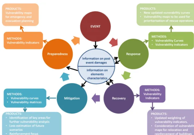
Figure 9.The role of vulnerability assessment and the corresponding methodological concepts in the phases of the disaster cycle (Papathoma-Köhle and Ciurean, 2014).
disaster cycle, highlighting the relevant methods for each phase. For example, during the mitigation phase vulnerabil-ity curves may be used for the loss estimation of future events and the design of mitigation measures. The results in this case may be used for public awareness and education as well as for recommendations for reinforcement. However, vulner-ability maps based on the vulnervulner-ability indicators may guide the emergency and evacuation planning process during the preparedness phase. Additionally, during the response phase, vulnerability maps are essential to indicate the buildings that are more likely to have been damaged, whereas the recovery phase is the ideal phase for validating the weighting of in-dicators. Moreover, during the recovery phase the results of the vulnerability assessment may be used as guidance for re-location of buildings. The centre of the disaster management cycle consists of an information pool including two types of data: empirical data from past events and an inventory of the elements at risk and their characteristics. The exchange of information between the pool and the different phases of the disaster cycle is also demonstrated in Fig. 9 through the black arrows.
In short, decision makers, authorities and disaster man-agers need a quantitative representation of physical vulner-ability based on empirical data (curves) as well as relative vulnerability values for individual elements that are directly connected to their characteristics (indicators) and may sup-port prioritisation of resources and small local interventions for vulnerability reduction. The fact that both approaches are significant stresses the need for a “holistic physical vulner-ability framework for practitioners” that will enable
practi-tioners not only to choose the relevant method according to their aim and the available resources but also to make full use of the fact that they both complement each other.
The interactions and possibilities for combination of the approaches should be included in a “holistic physical vulner-ability framework for practitioners” (Fig. 10).
Figure 10.A preliminary framework for the assessment of physical vulnerability (adapted for debris flow hazards) showing clearly the need for exchange and interaction between the two methodological approaches.
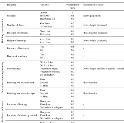
Table 4.Indicators for a scenario of 1.5 m debris height intensity and flow coming from the slope and not the river side.
Indicator Variable Vulnerability Justification of score score
Building
characteristics
Material
Adobe 1
Expert judgement Brick 0.5 0.5
Reinforced 0.1 0.1
Number of floors One floor 0.7 Debris height (scenario)
<One floor 0.1
Presence of openings Slope side 0.9 Flow direction (scenario) River side 0.2
Height of openings h <1.5 m 0.9 Debris height (scenario)
h >1.5 m 0.1
Presence of basement Yes 0.8 – No 0.2
Basement windows Yes 1 0.9 – No 0 0.1
Indicators
concerning
intensity Surroundings
Wall>1.5 m 0.1
Debris height and flow direction (scenario) Wall<1.5 m 0.3
Vegetation (trees) 0.5 Vegetation (bushes) 0.7 No protection 0.9
Building row towards river
First 0.3
Flow direction Second 0.3
>Third 0.3
Building row towards slope
First 0.9
Flow direction Second 0.7
>Third 0.4
Resilience
indicators
Location of heating
Basement 0.9 – First floor 0.5 Second floor or higher 0.1
Location of electricity central
Basement 0.9 – First floor 0.5 Second floor or higher 0.1
not only the debris height per building but also the direction of the flow and, ideally, the impact pressure or the velocity of the flow. This is the first “interaction” between the two sides (1). Information on the intensity of the event is also used to inform the group of indicators related to the inten-sity (2). The scores of the variables for each indicator will be formed according to the scenario as it is indicatively demon-strated in Table 4. In the same way, exchange of information is necessary in the other direction. Information regarding the buildings is also needed for the development of a vulnera-bility curve since data concerning the size and the value of the building are necessary for the calculation of the degree of loss (3). By using a specific scenario, the calculation of the IBM is not anymore intensity independent and the prediction capability of the method increases. Moreover, in contrast to the curves, additional information on the process, such as the flow direction, may be used.
The framework of Fig. 10 could be further improved by in-cluding more detailed information about their weighting and their aggregation to an index, possibilities for the identifica-tion of uncertainties and their quantificaidentifica-tion, as well as the consequences of change (climate and socioeconomic to both sides of the framework).
8 Conclusions
Vulnerability assessment constitutes a large part of risk anal-ysis and its reduction has a direct effect on the consequences of natural disasters on lives, livelihoods, communities, build-ings and infrastructure. The various methods available are used mostly until now in isolation. In this article, an IBM methodology is applied and scrutinised, enabling the com-parison between two large groups of approaches. The vulner-ability curves, although widely used by practitioners reveal the need to include the characteristics of the buildings (indi-cators) in the assessment of physical vulnerability. However, the IBM presented and applied in the present article shows that although assessing physical vulnerability using indica-tors may give reliable results, significant work has to be done in order to improve the use of IBMs for physical vulnera-bility assessment. Finally, the article emphasises that there is no need for new methodologies as far as the assessment of physical vulnerability is concerned. In contrast, there is a need not only to improve the existing ones but also to com-bine them in order to exploit their full power. The need for a “holistic framework for physical vulnerability assessment for practitioners” is emphasised and a preliminary version of this framework is presented. The framework offers the oppor-tunity to the end users to use both methodologies in a com-plementary way; however, in the future it should include ad-ditional steps for the quantification of uncertainties and the consideration of change, not only as far as the natural pro-cess is concerned (climate change) but also socioeconomic
and land use changes that will have a direct influence on the consequences of natural hazards.
Acknowledgements. This project received funding from the Austrian Science Fund (FWF): P 27400. Data collection was partly supported by the EU project MOVE (Methods for the Improvement of Vulnerability Assessment in Europe) (contract number 211590). The author would like to thank the Local Authorities of Bolzano and the Municipality of Martell for the provision of data and photo-graphic material. Furthermore, Thomas Thaler and Sven Fuchs are thanked for the discussions on earlier drafts of the present article.
Edited by: T. Glade
Reviewed by: two anonymous referees
References
Adger, N. W., Brooks, N., Bentham, G., Agnew, M., and Eriksen, S.: New indicators of vulnerability and adaptive capacity, Tyndall Centre for Climatic Research, Tyndall, 2004.
Balica, S. F., Douben, N., and Wright, N. G.: Flood vulnerability in-dices at varying spatial scales, Water Sci. Technol., 60.10, 2571– 2580, 2009.
Barnett, J., Lambert, S., and Fry, I.: The Hazards of Indicators: In-sights from the Environmental Vulnerability Index, Ann. Assoc. Am. Geogr., 98, 102–119, 2008.
Barroca, B., Bernardara, P., Mouchel, J. M., and Hubert, G.: In-dicators for identification of urban flooding vulnerability, Nat. Hazards Earth Syst. Sci., 6, 553–561, doi:10.5194/nhess-6-553-2006, 2006.
Birkmann, J.: Indicators and criteria for measuring vulnerability: Theoretical bases and requirements, in: Measuring Vulnerability to Natural Hazards: Towards disaster resilient societies, edited by: Birkmann, J., UNU Press, Tokyo, 2006.
Cutter , S., Boruff, B. J., and Shirley, W. L.: Social Vulnerability to Environmental Hazards, Social Sci. Quart., 84, 242–261, 2003. Dall’Osso, F., Gonella, M., Gabbianelli, G., Withycombe, G., and
Dominey-Howes, D.: A revised (PTVA) model for assessing the vulnerability of buildings to tsunami damage, Nat. Hazards Earth Syst. Sci., 9, 1557–1565, doi:10.5194/nhess-9-1557-2009, 2009a.
Dall’Osso, F., Gonella, M., Gabbianelli, G., Withycombe, G., and Dominey-Howes, D.: Assessing the vulnerability of buildings to tsunami in Sydney, Nat. Hazards Earth Syst. Sci., 9, 2015–2026, doi:10.5194/nhess-9-2015-2009, 2009b.
Dall’Osso, F., Maramai, A., Graziani, L., Brizuela, B., Cavalletti, A., Gonella, M., and Tinti, S.: Applying and validating the PTVA-3 Model at the Aeolian Islands, Italy: assessment of the vulnerability of buildings to tsunamis, Nat. Hazards Earth Syst. Sci., 10, 1547–1562, doi:10.5194/nhess-10-1547-2010, 2010. Dominey-Howes, D. and Papathoma, M.: Validating the Papathoma
Tsunami Vulnerability Assessment Model (PTVAM) using field data from the 2004 Indian Ocean tsunami, Nat. Hazards, 53, 43– 61, 2007.
Eidsvig, U. M. K., Papathoma-Köhle, M., Du, J., T., G., and Van-gelsten, B. V.: Quantification of model uncertainty in debris flow vulnerability assessment, Eng. Geol., 181, 15–26, 2014. Fell, R. and Hartford, D.: Landslide Risk Management, in:
Land-slide Risk Assessment, edited by: Cruden, D. M. and Fell, R., Balkema, Rotterdam, 1997.
Fuchs, S.: Susceptibility versus resilience to mountain hazards in Austria – paradigms of vulnerability revisited, Nat. Hazards Earth Syst. Sci., 9, 337–352, doi:10.5194/nhess-9-337-2009, 2009.
Fuchs, S., Heiss, K., and Hübl, J.: Towards an empirical vulner-ability function for use in debris flow risk assessment, Nat. Hazards Earth Syst. Sci., 7, 495–506, doi:10.5194/nhess-7-495-2007, 2007.
Fuchs, S., Kuhlicke, C., and Meyer, V.: Vulnerability to natural haz-ards – the challenge of integration, Nat. Hazhaz-ards, 58, 609–619, 2011.
Fuchs, S., Birkmann, J., and Glade, T.: Vulnerability assessment in natural hazard and risk analysis: current approaches and future challenges, Nat. Hazards, 64, 1969–1975, 2012.
Fuchs, S., Keiler, M., Sokratov, S. A., and Shnyparkov, A.: Spa-tiotemporal dynamics: the need for an innovative approach in mountain hazard risk management, Nat. Hazards, 68, 1217– 1241, 2013.
Fuchs, S., Keiler, M., and Zischg, A.: A spatiotemporal multi-hazard exposure assessment based on property data, Nat. Haz-ards Earth Syst. Sci., 15, 2127–2142, doi:10.5194/nhess-15-2127-2015, 2015.
Gems, B., Mazzorana, B., Hofer, T., Sturm, M., Gabl, R., and Au-fleger, M.: 3-D hydrodynamic modelling of flood impacts on a building and indoor flooding processes, Nat. Hazards Earth Syst. Sci., 16, 1351–1368, doi:10.5194/nhess-16-1351-2016, 2016. Haigh, R.: Discussion paper: Developing a resilient built
environ-ment: post-disaster reconstruction as a window of opportunity, Kandy, 13–14 December 2010.
HAZUS: Multi-Hazard Loss Estimation Methodology Earthquake Model, HAZUS MH-MR2, User Manual, FEMA and NIBS, Washington, D.C., 2006.
Holub, M. and Fuchs, S.: Mitigating mountain hazards in Aus-tria – legislation, risk transfer, and awareness building, Nat. Hazards Earth Syst. Sci., 9, 523–537, doi:10.5194/nhess-9-523-2009, 2009.
Holub, M., Suda, J., and Fuchs, S.: Mountain hazards: reducing vul-nerability by adapted building design, Environ. Earth Sci., 66, 1853–1870, 2012.
Kappes, M., Papathoma-Köhle, M., and Keiler, M.: Assessing phys-ical vulnerability for multi-hazards using an indicator-based methodology, Appl. Geogr., 32, 577–590, 2012.
Karagiorgos, K., Thaler, T., Hübl, J., Maris, F., and Fuchs, F.: Multi-vulnerability analysis for flash flood risk management, Nat. Haz-ards, 82, S63–S87, 2016.
Kaswalder, C.: Schätzungsstudie zur Berechnung des Schadenspo-tentials bei Hochwasserereignissen durch die Rienz im Abschnitt Bruneck – St. Lorenzen, Autonome Provinz Bozen – Südtirol, Bozen, South Tyrol, 2009.
Keiler, M., Knight, J., and Harrison, S.: Climate change and geo-morphological hazards in the eastern European Alps, Philos. T. Roy. Soc. A, 368, 2461–2479, 2010.
Leone, F., Aste, J.-P., and Velasquez, E.: Contribution des con-stats d’ endommagement au developpement d’ une methodolo-gie d’evaluation de la vulnerabilite applique aux phenomenes de mouvements de terrain, Bulletin de l’ Association de Ge-ographes, Paris, 350–371, 1995.
Leone, F., Aste, J.-P., and Leroi, E.: L’evaluation de la vulnerabilite aux mouvements du terrain: Pour une meilleure quantification du risque, Revue de geographie Alpine, 84, 35–46, 1996.
Liu, X. and Lei, J.: A method for assessing regional debris flow risk: an application in Zhaotong of Yunnan province (SW China), Geomorphology, 52, 181–191, 2003.
Lo, W.-C., Tsao, T.-C., and Hsu, C.-H.: Building vulnerability to debris flows in Taiwan: a preliminary study, Nat. Hazards, 64, 2107–2128, 2012.
Martell: http://www.gemeinde.martell.bz.it/gemeindeamt/html/,
last access: 13 July 2013.
Mazzorana, B., Comiti, F., Scherer, C., and Fuchs, S.: Developing consistent scenarios to assess flood hazards in mountain streams, J. Environ. Manage., 94, 112–124, 2012.
Mazzorana, B., Hübl, J., and Fuchs, S.: Improving risk assess-ment by defining consistent and reliable system scenarios, Nat. Hazards Earth Syst. Sci., 9, 145–159, doi:10.5194/nhess-9-145-2009, 2009.
Mazzorana, B., Simoni, S., Scherer, C., Gems, B., Fuchs, S., and Keiler, M.: A physical approach on flood risk vulnera-bility of buildings, Hydrol. Earth Syst. Sci., 18, 3817–3836, doi:10.5194/hess-18-3817-2014, 2014.
Müller, A., Reiter, J., and Weiland, U.: Assessment of urban vulner-ability towards floods using an indicator-based approach – a case study for Santiago de Chile, Nat. Hazards Earth Syst. Sci., 11, 2107–2123, doi:10.5194/nhess-11-2107-2011, 2011.
Papathoma, M. and Dominey-Howes, D.: Tsunami vulnerability as-sessment and its implications for coastal hazard analysis and disaster management planning, Gulf of Corinth, Greece, Nat. Hazards Earth Syst. Sci., 3, 733–747, doi:10.5194/nhess-3-733-2003, 2003.
Papathoma, M., Dominey-Howes, D., Zong, Y., and Smith, D.: As-sessing tsunami vulnerability, an example from Herakleio, Crete, Nat. Hazards Earth Syst. Sci., 3, 377–389, doi:10.5194/nhess-3-377-2003, 2003.
Papathoma-Köhle, M. and Ciurean, R.: Integrating physical vulner-ability models in a holistic framework- a tool for practicioners, Geophys. Res. Abstr., 16, EGU2014-3459, 2014.
Papathoma-Köhle, M., Neuhäuser, B., Ratzinger, K., Wenzel, H., and Dominey-Howes, D.: Elements at risk as a framework for assessing the vulnerability of communities to landslides, Nat. Hazards Earth Syst. Sci., 7, 765–779, doi:10.5194/nhess-7-765-2007, 2007.
Papathoma-Köhle, M., Kappes, M., Keiler, M., and Glade, T.: Phys-ical vulnerability assessment for alpine hazards:state of the art and future needs, Nat. Hazards, 58, 645–680, 2011.
Papathoma-Köhle, M., Totschnig, R., Keiler, M., and Glade, T.: Improvement of vulnerability curves using data from extreme events, Nat. Hazards, 64, 2083–2105, 2012.
Pfitscher, A.: Wasserkatastrophen in Martelltal – Der 24./25. Au-gust 1987, Municipality Martell, Martell, 1996.
Quan Luna, B., Blahut, J., van Westen, C. J., Sterlacchini, S., van Asch, T. W. J., and Akbas, S. O.: The application of numer-ical debris flow modelling for the generation of physnumer-ical vul-nerability curves, Nat. Hazards Earth Syst. Sci., 11, 2047–2060, doi:10.5194/nhess-11-2047-2011, 2011.
Rheinberger, C. M., Romang, H. E., and Bründl, M.: Proportional loss functions for debris flow events, Nat. Hazards Earth Syst. Sci., 13, 2147–2156, doi:10.5194/nhess-13-2147-2013, 2013.
Romang, H.: Wirksamkeit und Kosten von
Wildbach-Schutzmassnahmen, Verlag des Geographischen Instituts
der Universität Bern, Bern, 2004.
Scheer, S., Gardi, A., Guillande, R., Eftichidis, G., Varela, V., and de Vanssay, B.: Handbook of Tsunami Evacuation Planning Eu-ropean Union, JRC, Ispra, Italy, 2011.
Silva, M. and Pereira, S.: Assessment of physical vulnerability and potential losses of buildings due to shallow slides, Nat. Hazards, 72, 1029–1050, 2014.
Sterlacchini, S., Frigerio, S., Giacomelli, P., and Brambilla, M.: Landslide risk analysis: a multi-disciplinary methodolog-ical approach, Nat. Hazards Earth Syst. Sci., 7, 657–675, doi:10.5194/nhess-7-657-2007, 2007.
Tarbotton, C., Dominey-Howes, D., Goff, J. R., Papathoma-Köhle, M., Dall’Osso, F., and Turner, I. L.: GIS-based techniques for assessing the vulnerability of buildings to tsunami: current ap-proaches and future steps, in: Natural Hazards in the Asia-Pacific Region: recent advances and Emerging Concepts, edited by: Terry, J. P. and Goff, J., Geologicaol Society, London, 2012. Tarbotton, C., Dall’Osso, F., Dominey-Howes, D., and Goff, J.: The
use of empirical vulnerability functions to assess the response of buildings to tsunami impact: comparative review and summary of best practice, Earth-Sci. Rev., 142, 120–134, 2015.
Thaler, T. and Levin-Keitel, M.: Multi-level stakeholder engage-ment in flood risk manageengage-ment – a question of roles and power: Lessons from England, Environ. Sci. Policy, 55, 292–301, 2016. Thaler, T., Priest, S., and Fuchs, S.: Evolving interregional co-operation in flood risk management: distances and types of pert-nership approaches in Austria, Reg. Environ. Change, 16, 841– 853, 2016.
Totschnig, R. and Fuchs, S.: Mountain torrents: quantifying vulner-ability and assessing uncertainties, Eng. Geol., 155, 31–44, 2013. Totschnig, R., Sedlacek, W., and Fuchs, S.: A quantitative vulner-ability function for fluvial sediment transport, Nat. Hazards, 58, 681–703, 2011.
UN: Hyogo Framework for Action 2005–2015: Building the Re-silience of Nations and Communities to Disasters, Kyoto, Japan, 2007.
UNDRO: Disaster Prevention and mitigation-a compendium of cur-rent knowledge, UN, New York, 1984.
UNISDR: UNISDR Terminology on Disaster Risk Reduction, UN, Geneva, Switzerland, 2009.
Velotti, L., Trainor, J. E., Engel, K., Torres, M., and Myamoto, T.: Beyond vertical evacuation: research considerations for a com-prehensive “vertical protection srategy”, Int. J. Mass Emerg. Dis-ast., 31, 60–77, 2013.
Zanchetta, G., Sulpizio, R., Pareschi, M. T., Leoni, F. M., and San-tacroce, R.: Characteristics of May 5–6, 1998 volcaniclastic de-bris flows in the Sarno area (Campania, southern Italy): rela-tionships to structural damage and hazard zonation, J. Volcanol. Geoth. Res., 133, 377–393, 2004.