Dye Concentrations Determination in Ternary Mixture Solution by Using Colorimetric Algorithm

(1)

Dye Concentrations Determination

in Ternary Mixture Solution by Using Colorimetric

Algorithm

Shams-Nateri, Ali*

+

Textile Engineering Department, University of Guilan, Rasht, I.R. IRAN

ABSTRACT: This publication uses a colorimetric method based on the absorbance spectra of dye solutions to improve on Beer’s law when calculating the dye concentrations of a three-component mixture. The performance of the new method is compared with that of Beer’s law evaluated at three wavelengths, and Beer’s law evaluated at 16 wavelengths. Colorimetric method gives the best prediction of dye concentrations: the average relative errors in its predictions of the blue, red, and yellow concentrations are 55.64%, 12.3% and 14.84% respectively for new test solutions. Its average ternary relative error is 11.68% which is comparable to 14.31% for Beer’s law at three wavelengths.

KEY WORDS: Colorimetric algorithm, Beer’s law, Dye concentration, Absorbance spectra, Prediction.

INTRODUCTION

The transmission of monochromatic radiation through a dye solution is governed by Beer & Lambert’s law, which essentially states that the absorption of light is proportional to the number of absorbing molecules in its path. This theory can also be used when more than one kind of absorbing mater is present. Beer & Lambert’s Law (henceforth referred to as Beer’s Law for brevity) is written as

0

I

A Log L C

I

= = ε × × (1)

where A is the absorbance; Io is the original intensity

of the light beam; I is the intensity of the beam after passing through the sample; is the absorptivity, which depends on the absorbing molecule and the wavelength; L is the distance light travels through the sample, or path length; and C is the concentration.

All multi-component, quantitative dye models are based on the principle that the absorbance of a mixture is equal to the sum of the absorbance of its components. This is true at any given wavelength, although the relative importance of the components can vary with wavelength as changes. The concentrations do not change, however, and can be determined with sufficient data.

Absorbance measurements are widely used, through the application of Beer’s Law, for determining the amount of colorants in a solution. For example, this technique can be used to quantify the strength of a dye. Beer’s law is not perfect, however; there are actually several instrumental and chemical factors that can cause it to deviate from a simple linear form. A chemical deviation might be due to changes in the solubility of the absorbers, due to aggregation or other dye-dye interactions. In addition, the analysis of dye mixtures is often less accurate than that of single-dye solutions [1-9].

*To whom correspondence should be addressed.

+E-mail: [email protected]

(2)

Color matching is defined as a procedure of adjusting a color mixture until difference from a target is eliminated. Colorants formulation method is used to calculating the approximate colorant proportion to match a given object color. The most commonly used method for computer match prediction is colorimetric and spectrophotometric algorithms. In spectrophotometric algorithm, the reflectance spectra of the target and the sample will be matching at all wavelengths. Colorimetric method tray to minimize the differences X, Y, Z between target and sample. One of the most widely Known of colorimetric technique is the algorithm of Allen. In 1966, Allen explained a successful algorithm for determining the starting recipe, and this has been widely adopted [1, 10]. Allen reasoned that to achieve a tristimulus match we must solve three nonlinear simultaneous equations in three unknowns, the dye concentrations c1, c2 and c3 (Equation 2):

1 1 2 3 2 1 2 3 3 1 2 3

X g (c , c , c ) Y g (c , c , c ) Z g (c , c , c )

= = =

(2)

Where g1, g2 and g3 represent certain nonlinear

functions of the dye concentrations.

The V, T, E, R and p matrices are first defined (Eq. (3)):

X

V Y

Z

=

400 700 400 700 400 700

x ...x T y ...y z ...z

=

400 420

700

E 0 .... 0

0 E .... 0

E

... ... .... ...

0 0 ... E

=

t,400

t,700

R ... R

.... R

=

p,400

p,700

R

... P

.... R

= (3)

Where x, y and z are color matching function of the International Commission on Illumination (CIE) standard observer, E is the relative Spectral Power Distribution (SPD) of the specified light source, Rt is reflectance of the target

to be matched, Rp is reflectance of the

computer-predicted recipe and subscripts 400... represent wavelength in nm.

For a perfect match under a known illuminant, Eq. (4) holds:

T E P× × = × ×T E R (4)

And therefore (Eq. 5)

T E (P T)× × − =0 (5)

Allen assumes as an approximation a constant rate of change of f(R) with reflectance over the small difference between the target and the prediction. Eq. (6) can be written with a fair degree of accuracy:

t p

R −R = ∆Rλ

[

]

dR

f (R ) d f (R )_λ λ

λ

= × ∆

[

]

t, p,

dR

(f (R ) f (R ))

d f (R )λ λ λ

λ

= × − (6)

We can also define the matrices given in Eq. (7):

400 420

700

d 0 .... 0 0 d .... 0 D

... ... .... ... 0 0 ... d

=

t,400

t,700

f (R ) ... F

.... f (R )

=

p,400

p,700

f (R )

... G

.... f (R )

= (7)

We can now write Rt – Rp for all wavelengths as Eq. (8):

R−P=D (F G)× − (8)

Substituting Eq. (8) in Eq. (4), we obtain Eq. (9):

T E (F G)× × − =0 (9)

Transposing, we have Eq. (10):

T E D F× × × = × ×T E D G× (10)

(3)

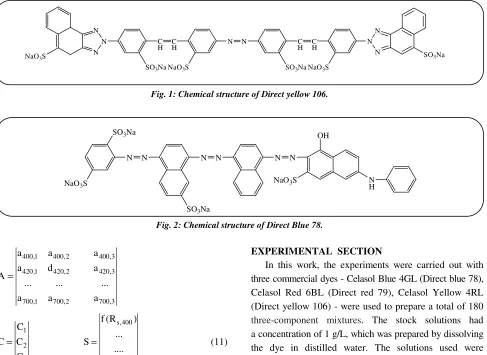
Fig. 1: Chemical structure of Direct yellow 106.

Fig. 2: Chemical structure of Direct Blue 78.

400,1 400,2 400,3 420,1 420,2 420,3

700,1 700,2 700,3

a a a

a d a

A

... ... ...

a a a

=

1 2 3

C C C C

=

s,400

s,700

f (R ) ... S

.... f (R )

= (11)

Where a400,1 is absorption coefficient at wavelength

400 nm of first dye, c1 = concentration of first dye, f(Rs, )

is Kubelka–Munk function of the substrate. Then, we can then write Eq. (12):

G= +S A C× (12)

Substituting Eq. 12 into Eq. 10 gives Eq. 13:

T E D F× × × = × × ×T E D (S A C)+ × (13)

Transposing gives Eq. 14:

T E D A C× × × × = × ×T E D (F S)× − (14)

Equation 13 now represents three linear equations in three unknowns (the dye concentrations), which can be solved by the usual calculation of the inverse matrix. Rearranging to obtain C results in Eq. 15 [1, 10-11]:

1

C=(T E D A)× × × − ×(T E D (F S))× × × − (15)

EXPERIMENTAL SECTION

In this work, the experiments were carried out with three commercial dyes - Celasol Blue 4GL (Direct blue 78), Celasol Red 6BL (Direct red 79), Celasol Yellow 4RL (Direct yellow 106) - were used to prepare a total of 180

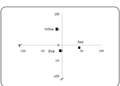
three-component mixtures. The stock solutions had a concentration of 1 g/L, which was prepared by dissolving the dye in distilled water. The solutions used were as follows: Direct blue 78 (0.0025, 0.05, 0.01, 0.015, 0.025 and 0.05 g/L), Direct red 79 (0.0005, 0.0025, 0.005, 0.0075, 0.025 g/L) Direct yellow 106 (0.01, 0.02, 0.05, 0.075, 0.1 and 0.125 g/L). The concentrations of dyes were chosen regarding to optimum values of absorbance maximum. The chemical structure of Direct yellow 106, Direct blue 78 and Direct red 79 are shown in Fig. 1, Fig. 2 and Fig. 3 respectively. Also, the absorbance spectra and the chromaticity diagram of dyes are shown in Figs. 4 and 5, respectively. Three-component mixture solutions were prepared from solution stock in a 100 mL volumetric flask. The full visible (380 to 700 nm) absorbance spectra of the solutions were measured by a CINTRA10- UV-Vis spectrophotometer.

One hundred samples were selected for calibration, and 80 samples were used to test its performance. Three different methods Beer’s law at three wavelengths, Beer’s law at 16 wavelengths, and the colorimetric methods were applied to these data, and their predictions of the dye concentrations based on the absorbance spectra of

N N N

C

H CH N N CH CH

NaO3S

SO3Na

NaO3S

SO3Na

N N N

SO3Na

N SO3Na

NaO3S

N N

SO3Na

N N N

OH

(4)

Fig. 3: Chemical structure of Direct red 79.

Fig. 4: The absorbance spectra of dyes (0.025 g/L Red, 0.025 g/L Blue, 0.05 g/L Yellow).

the mixtures were compared. The mathematical foundations of all four methods will be described below.

Beer’s law at three wavelengths

The three wavelengths selected are the wavelengths of maximum absorbance ( max) for each dye component.

Beer’s law gives the following three equations:

1 1 1 1

2 2 2 2

3 3 3 3

max1 1, 1 2, 2 3, 3

max 2 1, 1 2, 2 3, 3

max 3 1, 1 2, 2 3, 3

at A C C C

λ λ λ λ

λ = ε × + ε × + ε × λ = ε × + ε × + ε × λ = ε × + ε × + ε ×

(16)

where the subscripts are associated with the three components. Thus,

i j,λ

ε is the absorptivity of component j at the maximum absorption wavelength of component i.

Eq. 16 can be rewritten in matrix form:

1 1, 1 2, 1 3, 1 1

1 1, 2 2, 2 3, 2 2

1 1, 3 2, 3 3, 3 3

A C

λ λ λ λ

ε ε ε = ε ε ε ×

ε ε ε

(17)

Fig. 5:The chromaticity diagram of dyes (0.025 g/L Red,

0.025 g/L Blue, 0.05 g/L Yellow).

which in turn can be simplified to

A=MC (18) A is the vector of absorbances, M is the matrix of absorptivity coefficients, and C is the vector of dye concentrations.

The coefficients of M are determined from calibration samples by applying Eq. (19):

1

M=AC− (19) The concentrations in an unknown solution are then calculated as

1

C=M A.− (20)

Beer’s law at 16 wavelengths

The absorbance spectrum of the mixture is measured at 16 wavelengths between 400 nm and 700 nm (20 nm intervals). Beer’s law results in 16 equations within the visible spectrum:

N N

H3C

NaO3S

OH

NaO3S

OCH3

NHCONH

H3CO

CH3

N N

SO3Na

(5)

400 1,400 1 2,400 2 3,400 3 420 1,420 1 2,420 2 3,420 3

700 1,700 1 2,700 2 3,700 3

A C C C

. .

A C C C

= ε × + ε × + ε × = ε × + ε × + ε ×

= ε × + ε × + ε ×

(21)

Again, ε_j,λ is the absorptivity of component j at wavelength and C is the concentration of component j. _j

Eq. (21) can be rewritten in matrix form:

1,400 2,400 3,400 400

1,420 2,420 3,420 420

1 2 3

1,700 2,700 3,700 700 A A C . . . . C . . . . C . . . . A ε ε ε ε ε ε = × ε ε ε (22) or equivalently

A=QC (23) Note that unlike M, the matrix Q is not square. The coefficients of Q are determined from the absorbance spectra of known calibration samples using Eq. (24):

1

Q=AC− (24) Subsequently, the dye concentrations are calculated by Eq. (25):

1

C=Q A− (25)

Colorimetric method

In this method, the concentrations of the colorants are determined such that:

p t t p t _p X X Y Y Z _Z

= (26)

Where Xt, Yt and Zt are the tristimulus values of the

target solution and Xp, Yp and Zp are the tristimulus

values of a previously matched (known) sample under D65 illuminant and a standard colorimetric observer. The tristimulus values can be calculated from the transmittance spectra of a three-component mixture by Eqs. (27-29):

100

X E T x

K _λ λ λ λ

= × × (27)

100

Y E T y

K _λ λ λ λ

= × × (28)

100

Z E T z

K _λ λ λ λ

= × × (29)

Where Tλ is the transmittance value at wavelength , Eλ is the spectral power distribution of the D65 illuminant at wavelength , and x , y , zλ λ λ are the color-matching functions of the 10° standard colorimetric observer at wavelength . The parameter K is defined as E y_λ _λ

λ .

Eq. (26) is extended to Equation 30 by substitution of Eqs. (27-29):

t p

NET =NET (30) Where N, E, Tt and Tp are defined as follows:

400 420 700

x x . . . x

N y y . . . y

z z . . . z

= (31)

400 420

680 700

E 0 0 0 0 0 0

0 E 0 0 0 0 0

0 0 . 0 0 0 0

E 0 0 0 . 0 0 0

0 0 0 0 . 0 0

0 0 0 0 0 E 0

0 0 0 0 0 0 E

= (32)

t,400 t,420 t t,700 T T . T . . T

= (33)

p,400 p,420 p p,700 T T . T . . T

(6)

Equation 30 can be rewritten as

t p

NE(T −T )=0 (35) where 0 is the zero vector. If the first dye concentration is changed by a small amount c1,

the tristimulus values would change as follows:

1 1 1 1 1 X X C C1 Y Y C C Z Z C C ∂ ∆ = × ∆ ∂ ∂ ∆ = × ∆ ∂ ∂ ∆ = × ∆ ∂ (36)

If all three dye concentrations are changed by the small amounts c1, c2 and c3, the consequent changes

in X, Y and Z are the sum of the individual changes calculated using Eq. (37):

1 2 3

X X X

X C C C

C C C

Y Y Y

Y C C C

C C C

Z Z Z

Z C C C

C C C

∂ ∂ ∂ ∆ = × ∆ + × ∆ + × ∆ ∂ ∂ ∂ ∂ ∂ ∂ ∆ = × ∆ + × ∆ + × ∆ ∂ ∂ ∂ ∂ ∂ ∂ ∆ = × ∆ + × ∆ + × ∆ ∂ ∂ ∂ (37)

Furthermore, the partial derivatives of X can be obtained by Eq. (25) (the partials of Y and Z are obtained similarly): i i T X E x C C λ λ λ λ ∂ ∂ = × ×

∂ ∂ (38)

or equivalently i i i i i i T A X E x

C A C

T A

Y

E y

C A C

T A

Z

E z

C A C

λ λ λ λ λ λ λ λ λ λ λ λ λ λ λ λ λ λ ∂ ∂ ∂ = × × × ∂ ∂ ∂ ∂ ∂ ∂ = × × × ∂ ∂ ∂ ∂ ∂ ∂ = × × × ∂ ∂ ∂ (39)

From Beer-Lambert’s law:

1, 2, 3,

1 2 3

A A A

, ,

C C C

λ λ λ

∂ ∂ ∂

= ε = ε = ε

∂ ∂ ∂ (40)

Returning to Eq. (35), we can write the difference in transmittance vectors as

t p t, p,

T T

T T T A (A A )

A A λ λ

∂ ∂

− = ∆ = × ∆ = × −

∂ ∂ (41)

A

T=10− (42) We now define

A

dT

d 1 ln(10) 10

dA

λ

λ −

λ λ

= = − × × (43)

and

400 420

680 700

d 0 0 0 0 0 0

0 d 0 0 0 0 0

0 0 . 0 0 0 0

D 0 0 0 . 0 0 0

0 0 0 0 . 0 0

0 0 0 0 0 d 0

0 0 0 0 0 0 d

= (44)

allowing us to write

(

)

t p t p

T −T =D A −A (45)

Finally, Eq. (35) becomes

t p

NED(A −A )=0 (46)

which leads to

t

NED(A − φC)=0 (47)

Theφ matrix is defined by Eq. (48):

1,400 2,400 3,400 1,420 2,420 3,420

1,700 2,700 3,700

. . . . . . . . . ε ε ε ε ε ε φ = ε ε ε (48)

Therefore, the dye concentrations are determined by Eq. (49):

(

)

1

(

)

t

(7)

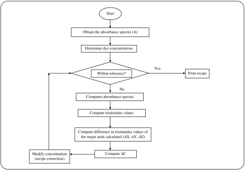
Fig. 6: The flow chart of colorimetric method.

correction of initial result is carried out by iteration technique. In this method, the change of tristimulus values with change of concentration of each component were used to correct the initial concentration (Eq. (50)).

(

)

1

C NED − T

∆ = φ (50) Were C and T vectors are obtained by Eqs.(51)and (52):

1 2 3

C

C C

C

∆ ∆ = ∆ ∆

(51)

X

T Y

Z

∆ = ∆ ∆

(52)

Where T represents differences in tristimulus values of the target and calculated formula.

The correction to the initial predicted recipe is done by Eq. (53).

1 1

2 2

3 3

C C

C C C

C C

+ ∆ = + ∆ + ∆

(53)

The flow chart of colorimetric method is shown in Fig. 6.

RESULTS AND DISCUSSION

This work compares the performance of all three methods in determining the dye contents of three-component mixtures starting from their observed absorbance spectra. The absorbance spectra of 180 different mixtures were divided into two samples: a training set with 100 spectra and a test dataset with 80 spectra.

The relative error (Er) and ternary relative error (Etr)

of each test result are calculated by Eq. (54) and Eq. (55) respectively:

a p

r

a

C C

E 100

C

−

= × (54)

Start

Obtain the absorbance spectra (A)

Determine dye concentrations

Print recipe Within tolerance?

Computer absorbance spectra

Compute tristimulus values

Compute difference in tristimulus values of the target ande calculated (∆X, ∆Y, ∆Z)

Compute ∆C Modify concentration

(recipe correction)

Yes

(8)

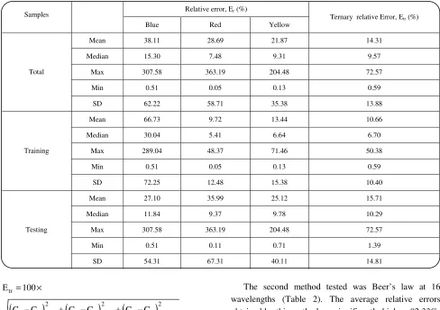
Table 1: Errors in dye concentration prediction by Beer’s law at 3 wavelengths.

Relative error, Er (%)

Samples

Blue Red Yellow

Ternary relative Error, Etr (%)

Mean 38.11 28.69 21.87 14.31

Median 15.30 7.48 9.31 9.57

Max 307.58 363.19 204.48 72.57

Min 0.51 0.05 0.13 0.59

Total

SD 62.22 58.71 35.38 13.88

Mean 66.73 9.72 13.44 10.66

Median 30.04 5.41 6.64 6.70

Max 289.04 48.37 71.46 50.38

Min 0.51 0.05 0.13 0.59

Training

SD 72.25 12.48 15.38 10.40

Mean 27.10 35.99 25.12 15.71

Median 11.84 9.37 9.78 10.29

Max 307.58 363.19 204.48 72.57

Min 0.51 0.11 0.71 1.39

Testing

SD 54.31 67.31 40.11 14.81

tr

E =100×

(

)

(

)

(

)

( )

2 2 2

a p _Red a p _Blue a p _Yellow

2 2 2

a Red a Blue a Yellow

C C C C C C

C C C

− + − + −

+ + (55)

where Ca is the actual concentration value and Cp is

the predicted concentration value. Note that the first error is calculated independently for each color of dye.

First the concentrations were evaluated by Beer’s law at three wavelengths: 555nm, 495nm, and 400 nm. These are the wavelengths of maximum absorbance for the blue, red and yellow dyes respectively. The results obtained from the total, training, and test samples are shown in Table 1. The average relative errors (Er) in the entire

samples are 38.11%, 28.69% and 21.87% for blue, red and yellow components respectively. The average relative errors in the training samples are 66.73%, 9.72% and 13.44% for the blue, red and yellow components respectively. The average relative errors in the test sample are 27.1%, 35.99% and 25.12%, in the same order. The average ternary relative errors (Etr) of the total,

training and test samples are14.31, 10.66% and 15.71% respectively.

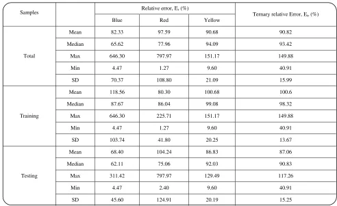
The second method tested was Beer’s law at 16 wavelengths (Table 2). The average relative errors obtained by this method are significantly higher: 82.33%, 97.59% and 90.68% in the total sample, 118.56%, 80.30% and 100.68% in the training sample and 68.40%, 104.24% and 86.83% in the test sample. The ternary relative errors in the total, training and testing samples averaged 90.82, 100.06% and 87.06% respectively.

In spectroscopy measurement, the Beer’s law as common linear relationship states that the absorbance is directly proportional to concentration. The linearity of absorbance spectra is dependent on wavelength. The best calibration in terms of linearity is obtained at the wavelength of maximum absorbance at which the correlation coefficient approaches unity. Correlation coefficient of zero indicates that there is no correlation between absorbance and concentration. In this, the error of concentration prediction is highest than the wavelength of maximum absorbance. Then, the calculation of dye concentrations at three wavelengths (Beer’s law) produces smaller error compared to that at 16 wavelengths.

(9)

Table 2: Errors in dye concentration prediction by Beer’s law at 16 wavelengths..

Samples

Blue Red Yellow

Mean 82.33 97.59 90.68 90.82

Median 65.62 77.96 94.09 93.42

Max 646.30 797.97 151.17 149.88

Min 4.47 1.27 9.60 40.91

Total

SD 70.37 108.80 21.09 15.99

Mean 118.56 80.30 100.68 100.6

Median 87.67 86.04 99.08 98.32

Max 646.30 225.71 151.17 149.88

Min 4.47 1.27 9.60 40.91

Training

SD 103.74 41.80 20.25 13.67

Mean 68.40 104.24 86.83 87.06

Median 62.11 75.06 92.03 90.83

Max 311.42 797.97 129.49 117.26

Min 4.47 2.40 9.60 40.91

Testing

SD 45.60 124.91 20.19 15.25

tristimulus values of the target solution to known samples described using Beer’s Law at 16 wavelengths. The approach is similar to the usual single-constant colorimetric match prediction algorithm. The average relative errors in the total samples are 55.44%, 12.38% and 15.27% for blue, red and yellow components, respectively. The average relative errors in the training samples are 112.58%, 11.39% and 20.44% for blue, red and yellow components, respectively. The average relative errors in the test samples are 33.46%, 12.76% and 13.28% for blue, red and yellow dyes, respectively. The ternary relative errors are 12.1, 15.65% and 10.73% for the total, training and test samples respectively. Afterward, the initial predicted concentration is corrected by using iteration technique (Eq. (53)). Table 4 shows the obtained results in computer iteration technique. As shown in this Table, the average relative errors for the total samples are 55.64%, 12.03% and 14.84% for blue, red and yellow components, respectively. The average relative errors for the training samples are 61.71%, 15.08% and 17.15% for blue, red and yellow components, respectively. The average relative errors for the test samples are 48.05%, 8.21% and 11.95% for blue,

red and yellow components, respectively. The ternary relative errors are quite good, averaging 11.68 %, 12.86% and 10.22% for the total, training and test samples respectively.

CONCLUSIONS

(10)

Table 3: Errors in dye concentration prediction by the colorimetric method.

Samples

Blue Red Yellow

Mean 55.44 12.38 15.27 12.1

Median 19.26 6.81 7.85 7.62

Max 519.58 177.26 106.77 58.27

Min 0.08 0.10 0.02 0.33

Total

SD 99.12 20.81 18.25 12.38

Mean 112.58 11.39 20.44 15.65

Median 56.08 8.70 11.57 10.12

Max 519.58 40.36 106.77 58.27

Min 0.08 0.10 0.02 0.33

Training

SD 129.22 9.56 24.76 16.15

Mean 33.46 12.76 13.28 10.73

Median 11.99 6.46 7.21 7.06

Max 430.90 177.26 69.72 44.52

Min 0.08 0.10 0.02 0.33

Testing

SD 74.42 23.78 14.65 10.33

Table 4: Errors in dye concentration prediction by the colorimetric method with correction iteration.

Samples

Blue Red Yellow

Mean 55.64 12.03 14.84 11.68

Median 19.67 7.05 7.10 7.19

Max 520.34 163.48 127.95 55.50

Min 0.08 0.12 0.12 0.32

Total

SD 99.47 18.55 19.36 11.57

Mean 61.71 15.08 17.15 12.86

Median 20.25 8.91 7.59 7.49

Max 520.34 163.48 127.95 55.50

Min 0.08 0.17 0.24 0.78

Training

SD 105.03 22.85 22.84 12.79

Mean 48.05 8.21 11.95 10.22

Median 19.26 5.49 6.62 6.61

Max 432.82 59.39 70.94 40.70

Min 0.51 0.12 0.12 0.32

Testing

(11)

improved by using computer iteration technique. Besides, the colorimetric method can be used to study the effect of nature and composition of dye solution, for example fluorescent and high concentration dye solutions, which caused shift of wavelength. So that, colorimetric algorithm decreases the effect of wavelength shifting on recipe prediction performance.

Received : May 1, 2010 ; Accepted : May 9, 2011

REFERENCES

[1] McDonald R., "Colour Physics for Industry", Society of Dyers and Colourists, (1997).

[2] Owen T., "Fundamentals of Modern UV-Visible Spectroscopy", Agilent Technologies, (2000). [3] Jasper W.J., Kovacs E.V., & Berkstresser G.I., Using

Neural Networks to Predict Dye Concentrations in Multiple-Dye Mixtures, Textile Researcher Journal., 63(9), p. 545 (1993).

[4] Marjoniemi M., Mantysalo E., Neuro-Fuzzy Modeling of Spectroscopic Data, Part A: Modeling of Dye Solutions, Journal of the Society of Dyers & Colourists., 113, p. 13 (1997).

[5] Marjoniemi M., Mantysalo E., Neuro-fuzzy Modeling of Spectroscopic Data, Part B: Dye Concentration Prediction, Journal of the Society of Dyers & Colourists, 113, p. 64 (1997).

[6] Gary N.M., "Modern Concepts of Color and Appearance", Science Publishers Inc. U.S.A, (2000). [7] Logan H., "UV and Visible Spectrophotometry in

Organic Chemistry". http://members.aol.com/ logan20/uv.html, (1997).

[8] Stearns E.I., "The Practice of Absorption Spectrophotometry", Wiley-Interscience, (1969). [9] Westland S., Ripamonti C., "Computational Colour

Science Using Matlab", John Wiley & Sons, Ltd, England, (2004).

[10] Allen E., Basic Equations Used in Computer Color Matching, Journal of the Optical Society America, 56, p. 1256 (1966).